DOI:
10.1039/D5LC00592B
(Paper)
Lab Chip, 2025,
25, 6442-6453
Continuous and tunable droplet splitting using standing-wave acoustofluidics
Received
16th June 2025
, Accepted 6th August 2025
First published on 12th August 2025
Abstract
Droplet splitting plays an important role in droplet microfluidics by providing precise control over droplet size, which is essential for applications such as single-cell analysis, biochemical reactions, and the fabrication of micro- and nanosized material. Conventional methods of droplet splitting using obstructions or junctions in the microchannel have a clear limitation that the split ratio for a particular device remains fixed, while existing active splitting methods are constrained by low flow rates, the need for complex systems, or limitations to specific droplet types. In this study, we demonstrate that droplet splitting can be achieved simply using a one-dimensional standing-wave field excited within a microchannel. The mechanism of droplet splitting is investigated using theoretical analysis, numerical simulations, and high-speed imaging. It is found that splitting occurs due to the opposing acoustic radiation pressure acting on the two sides of the droplet, when the droplet with a negative contrast factor is placed near the pressure node. The entire splitting process can be characterized by necking, full-stretch, and splitting regimes, and it is completed in approximately 1 ms or less, demonstrating the capability to perform in-flow droplet splitting at high throughput. Continuous droplet splitting is successfully performed at a flow rate of 161 μL min−1 with an equal split ratio, and at flow rates between 33.1 and 45.1 μL min−1 with unequal split ratios ranging from 0.27 to 0.7. Selective and controllable cross-phase particle manipulation is achieved through droplet splitting and subsequent acoustic actuation, thereby extending the capabilities of droplet microfluidics in microreactions and drug delivery.
1 Introduction
Droplet microfluidics enables the rapid generation and manipulation of discrete droplets within microchannels filled with multiphase flows.1 As an essential tool in microfluidics technology, it underpins diverse applications spanning biochemical assays,2,3 materials synthesis,4,5 high-throughput screening,6 single-cell analysis,7,8 and drug screening.9,10 The versatility of droplet platforms relies on integrated unit operations, including generation,11 sorting,12 merging,13 and splitting,14 which collectively enable complex fluidic workflows. In parallel with ongoing developments in droplet manipulation techniques, the scope of droplet microfluidics has expanded significantly into new application domains. Recent advances have highlighted its versatility in areas such as high-throughput screening, assisted reproduction, tissue engineering using microgel droplets, and single-cell analysis for omics and diagnostics.8,15–17 These emerging applications increasingly require precise, programmable, and scalable control over droplet operations, including splitting, which remains a key unit process for enabling parallelization, reagent partitioning, and conditional content release.
Among all the unit operations in droplet microfluidics, droplet splitting is critical as it enhances experimental capacity by increasing the number of compartments available for parallel reactions and analyses. In most studies, droplet splitting is achieved passively by introducing obstructions or junctions in the microchannel. However, a limitation of this approach is that the split ratio remains fixed for a given microchannel design. A recent study also reveals that the presence of the daughter droplets alter the flow resistance in different branches, causing the actual split ratio to differ from the designed one.18 To achieve a tunable split ratio with precise control, active droplet splitting utilizing external forces is required. Surprisingly, studies on this topic are limited, particularly in the context of droplet splitting within microchannels. Various active droplet splitting strategies, such as thermal, pneumatic, electric, and magnetic methods, have also been explored, each offering distinct advantages but often facing trade-offs in device complexity, throughput, or biocompatibility.
Acoustofluidics-based droplet manipulation has been demonstrated since the beginning of the field, with pioneering work on nanoliter droplet manipulation using surface acoustic waves (SAW).19 As a result, a wide range of studies have been conducted on droplet manipulation using acoustofluidic techniques, covering areas such as droplet generation,20,21 sorting,22–25 size modulation,26,27 merging,28–31 programmable manipulation,32 assembly,33 printing,34 ejection,35 and particle manipulation in droplets.36 However, the use of acoustofluidics for droplet splitting remains relatively unexplored,37,38 particularly when it comes to droplet splitting inside microchannels, which is essential for continuous processing in droplet microfluidic platforms. Inspired by previous works for acoustofluidic droplet generation,26,27 Jung et al. demonstrated on-demand droplet splitting in a microchannel using traveling SAW.38 By employing a slanted-finger interdigital transducer with an aperture width smaller than the droplet length, the droplet is compressed by the acoustic radiation force as it passes through the traveling SAW and subsequently split by the resulting acoustic gradient force along the flow direction. One major limitation of this technique is its low throughput, primarily due to the narrow beam width (100 μm) of the traveling SAW, which limits the amount of time the droplet is exposed to the sound field. Consequently, strong acoustic radiation and gradient forces are required to split droplets at high flow rates. Unfortunately, achieving this is challenging in SAW devices that use polydimethylsiloxane (PDMS) for microchannel fabrication, due to the similar acoustic impedance between PDMS and the surrounding medium. In the case of traveling SAW, it becomes even more difficult to generate a strong sound field due to the lack of resonance conditions in the channel.
Interestingly, droplet splitting using acoustic waves was first performed in the 1980s. By modulating the pressure amplitude in a standing-wave field with two superimposed frequencies, Marston and Apfel were able to experimentally achieve39 and theoretically explain40 large-amplitude droplet oscillations, ultimately leading to droplet splitting. This was later confirmed by two independent groups with high-speed imaging.41,42 While the droplet size in previous studies ranged from 1 mm to 12 mm, which is larger than those typically studies in droplet microfluidics, their works clearly indicate that droplet splitting is achievable in a standing-wave field. Here, we demonstrate continuous and tunable droplet splitting in a microchannel with a one-dimensional (1D) standing-wave field excited at a single frequency, without the need for amplitude modulation. While droplet splitting via this mechanism has been recently shown in a fundamental study under stop-flow conditions,43 applications leveraging this phenomenon remain unexplored. In this study, after elucidating the droplet splitting mechanism through high-speed imaging and numerical simulations, continuous droplet splitting is successfully demonstrated as a robust unit operation in droplet microfluidics at a flow rate of 161 μL min−1 with an equal split ratio, and at 33.1 to 45.1 μL min−1 with unequal split ratios. Building on this, we further achieve cross-phase manipulation of 20 μm and 40 μm-diameter polystyrene particles from the droplet phase to the continuous aqueous phase following droplet splitting. This enables selective and controllable particle release, an essential functionality for applications in microreactions and drug delivery systems.
2 Modelling
2.1 Governing equations
The acoustic radiation force exerted on a single spherical particle much smaller than the wavelength (Rayleigh particles) undergoing small deformations has been well established on a solid theoretical foundation, since the seminal works of Yosioka and Kawasima,44 as well as Gor'kov.45 However, droplet splitting in the context of droplet microfluidics involves droplets whose sizes are comparable to the acoustic wavelength (Mie particles), as well as large deformations. Several analytical and numerical models have been proposed to study deformable objects subject to acoustic radiation forces.46–49 While these methods efficiently simulate acoustic deformation, they often become inadequate when dealing with large deformations or changes in geometric topology due to the limitations of the models. For instance, in droplet splitting simulations, traditional moving mesh models may encounter issues such as grid mismatches and numerical instability, particularly at the moment of splitting. This can lead to grid distortion or even grid failure, potentially causing numerical instability or incorrect results.
Given that the droplet splitting involves significant deformations and topological changes, using a moving mesh method for grid handling introduces considerable complexity. In contrast, the volume of fluid (VOF) method, which employs a fixed Eulerian grid for interface tracking, does not require explicit geometric reconstruction of the interface. Instead, the interface is implicitly captured on the fixed grid, naturally appearing and disappearing. This characteristic helps mitigate the challenges associated with large deformations and topological changes of droplets.50 Therefore, in our model, we consider an incompressible, immiscible two-phase fluid system accounting for the interfacial tension, the governing equations for continuity, momentum, state, and transport are as follows
| | | ∂t(ρv) + ∇·(ρvv) = ∇·σ + f + Fst, | (1b) |
Here,
σ = −
pI +
μ(∇
v + (∇
v)
T) is the fluid stress tensor, and
f represents the body force. The interfacial force
Fst is given by
Fst =
![[small sigma, Greek, tilde]](https://www.rsc.org/images/entities/i_char_e10d.gif) κ
κ(
ϕ)
δ(
ϕ)∇
ϕ, where
,
κ, and
δ are the interfacial tension coeffcient, the curvature (which is defined only on surfaces or curves), and a Dirac delta function located at the interface, respectively. The curvature is computed using the volume fraction as
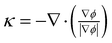
.
51 The isentropic compressibility is defined as
χ = (1/
ρc2), where
c is the speed of sound of the fluid. The fluid type in
eqn (1a)–(1d) is determined based on the value of the phase function
ϕ in each computational cell following
| | 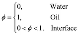 | (2) |
Acoustofluidic devices typically operate at MHz frequencies. For devices working at a frequency of 2 MHz, the acoustic time scale is approximately 0.5 μs, while the time scale for hydrodynamics or interface movement is significantly longer (around 100 μs, as observed in our experiments). This results in a difference of at least two orders of magnitude between the fast acoustic time scales and the slow hydrodynamic time scale. Moreover, during droplet deformation, the surface morphology undergoes significant changes, with interfacial tension playing a crucial role in this process. Given these characteristics, we adopt a time-scale separation approach and use an iterative numerical model52,53 to develop equations and models. The physical quantities are decomposed into hydrodynamic and acoustic fields as
| | | Q(X, t) = Q0(X, t) + Q1(X, t)eiωτ, | (3) |
where the subscripts 0 and 1 are defined as the hydrodynamic and acoustic fields, respectively. To describe the response of the acoustic field under the excitation of angular frequency
ω, the first-order field variables are treated as a time-harmonic disturbance on a fast time scale.
54
Due to the significant difference in time scales between the acoustic and flow fields, it can be assumed that the distribution of each component remains steady under the influence of the sound field. As a result, when calculating the acoustic field, the motion of the droplet boundary is neglected. At the fast time scale, by introducing the time-separated equations into the governing equations (eqn (1a)–(1d)), the zeroth-order equilibrium terms are eliminated. Based on the assumptions ρ1 ≪ ρ0, v0 < v1 ≪ c, the negligible terms are removed from the equations. Moreover, since  , the convective term is also discarded from the equations. Finally, by replacing all time-derivative terms ∂/∂τ with iω, the governing equation for the acoustic field is obtained as52,53,55–57
Here,
σ1 = −
p1I +
μ(∇
v1 + (∇
v1)
T).
The time-averaged value of a harmonic field over one oscillation period is zero. However, due to the nonlinear nature of the Navier–Stokes equations, the time average of the nonlinear terms becomes nonzero. As a result, over long time scales, the acoustic field generates a time-averaged acoustic radiation pressure on the droplet, which drives the motion of its boundary. By time-averaging eqn (1a)–(1d), the governing equations become
| | | ∂t(ρ0v0) + ∇·(ρ0v0v0) = ∇·σ0 + fac + Fst, | (5b) |
Here,
fac = −∇·〈
ρ0v1v1〉 represents the acoustic body force.
56,58 In addition to the terms with zero time-averaged quantities, the terms involving
ρ1v1 are also neglected, since
ρ1 and
v1 are π/2 out of phase in a one-dimensional standing-wave field.
2.2 Modelling setup
To study the dynamic splitting process of a spherical droplet in a standing-wave field, a numerical model was developed based on the governing equations described in Sec 2.1. This model was implemented using the finite element software COMSOL Multiphysics,59 with iteration and coupling handled in MATLAB through LiveLink™. While a complete three-dimensional (3D) model would be ideal to accurately capture the droplet splitting dynamics, the computational cost for a rectangular cavity is prohibitively high for a standard workstation. Therefore, a two-dimensional (2D) cylindrical coordinate system, symmetric with respect to the channel width direction, was adapted [as shown in Fig. 1(a)]. This approach accounts for both the acoustic scattering and the effect of 3D droplet curvature on interfacial tension, while minimizing computational cost. The computational domain had an area of 375 × 350 μm2. It should be noted that the top and bottom walls were present in our acoustofluidic devices, but these walls were not included in the 2D axisymmetric model (which assumes an infinite domain along the R-direction). During droplet splitting, fluid relocation interacts with both the modeled sidewalls and the unmodeled top and bottom walls. These solid boundaries can redirect the flow, which may in turn influence droplet deformation. However, such effects are transient and dissipate rapidly, they are considered negligible in the simulation.
 |
| | Fig. 1 (a) The 2D axisymmetric model used in this study. The cylindrical coordinate system is symmetric along the channel width, with the axis of symmetry indicated by the black dashed line. Velocity boundary conditions v1 = V1eiωτ are applied to the sidewalls (red arrows) to excite a half-wavelength standing-wave field along the axis of symmetry. A perfectly matched layer (PML) is placed at the outer boundary of the computational domain. (b) The computational mesh used in the model, with a zoomed-in view of the mesh configuration near the droplet interface. The mesh size is enlarged by a factor of five for better visualisation. | |
In this model, the Pressure Acoustics module was first used to calculate the acoustic field. Velocity boundary conditions v1 = V1eiωτ were applied to the sidewalls to excite a half-wavelength standing-wave field. To achieve a better quantitative match between the simulation and the experiment, V1 was adjusted to match the acoustic energy density Eac measured experimentally when the domain (channel) was filled only with water. The outer boundary of the computational domain was defined by a perfectly matched layer (PML), where the acoustic field was artificially damped to mimic an infinite domain. Next, the Two-phase Flow module was employed to model the motion of the droplet boundary, with the acoustic body force fac acting as a coupling term to represent the interaction between the acoustic and the phase fields. Finally, since the presence and shape of the Mie particle affect the acoustic field, a MATLAB code was used to update the distribution of the oil and water phases, which were then used for iterative calculation of the acoustic field. A mesh convergence test was performed in accordance with the methodology described by Muller et al.,55 with the results presented in Fig. S1 of the SI. The mesh used in the simulation is shown in Fig. 1(b), with the mesh size enlarged by a factor of five for better visualisation. It is important to note that acoustic streaming, including the boundary-driven streaming resulting from the acoustic energy decay on the channel (top and bottom) walls and on the droplet interface, was neglected for two reasons. First, the entire droplet splitting process occurs within a time scale (≈1 ms) during which boundary-driven acoustic streaming has not been fully developed.60,61 Second, the strong motion of the droplet also causes rapid fluid relocation, resulting in flow motion much faster than the boundary-driven acoustic streaming. All the material properties used in the model are summarized in Table 1.
Table 1 Fluid properties. All the properties were measured at 25 °C
| Water with 10 wt% Tween® 20 |
| Density |
1009.5 |
kg m−3 |
| Speed of sound |
1525.4 |
m s−1 |
| Dynamic viscosity |
1.81 |
mPa s |
| Fluorinated fluid |
| Density |
1621.0 |
kg m−3 |
| Speed of sound |
671.5 |
m s−1 |
| Dynamic viscosity |
1.24 |
mPa s |
| Interfacial tension coefficient at the |
12.4 |
mN m−1 |
| Water/fluorinated fluid interface |
|
|
| Mineral oil |
| Density |
858.1 |
kg m−3 |
| Speed of sound |
1450.8 |
m s−1 |
| Dynamic viscosity |
116.0 |
mPa s |
| Interfacial tension coefficient at the |
5.6 |
mN m−1 |
| Water/mineral oil interface |
|
|
3 Experimental
3.1 Acoustofluidic devices
Three acoustofluidic devices, each with identical chip and main channel dimensions, were used for stop-flow, in-flow, and cross-phase particle manipulation experiments, respectively. The microchannel was etched through the silicon layer using deep reactive-ion etching. The long, straight channel had dimensions of 50 × 0.375 × 0.2 mm3, as shown in Fig. 2(a). Trifurcations were fabricated at the ends of the straight channel, with all three branches at the trifurcation (one center channel and two side channels) featuring a linearly decreasing width [see Fig. 2(b) and (c)]. The center channel was widened at an 8-degree angle and connected to the main channel where the sound field was generated. The four orifices at the trifurcation of two devices had the same cross sectional area of 100 × 200 μm2, while the orifices of the third device had a cross sectional area of 200 × 200 μm2 to prevent particle clogging in cross-phase particle manipulation experiment. The silicon layer was bonded to two pyrex layers using anodic bonding, resulting in final chip dimensions of 70 × 3 × 1.2 mm3. Silicone tubing (outer diameter 3 mm, inner diameter 1 mm, length 7 mm) was attached to the inlets and outlets using silicone glue (ELASTOSIL® A07 TRANSLUCENT, Wacker Chemie, Munich, Germany). A single lead zirconate titanate (PZT) transducer was attached to one sidewall of the chip near the trifurcation to provide efficient actuation of the acoustofluidic device and generate a strong sound field in the channel.62 For the chip used in the stop-flow experiment, a PZT transducer with dimensions of 10 × 2 × 1 mm3 was used, while a shorter with dimensions of 5 × 2 × 1 mm3 was employed in the chip for the in-flow experiment. The dimensions of the transducer corresponded to its fundamental thickness mode at approximately 2 MHz, which matched the resonance frequency of a half-wavelength standing-wave field along the channel width (y-) direction when the channel was filled with water.
 |
| | Fig. 2 (a) The glass-silicon-glass sandwiched acoustofluidic device used in this study. Trifurcations with narrowed orifices were fabricated at both ends of the long straight channel. A PZT transducer (brown) was glued to the side of the device. (b) For droplet splitting with an equal split ratio, oil was infused through the center inlet, while water was infused through the side inlet. (c) For droplet splitting with unequal split ratios, water was infused through the center inlet, while oil was infused through the side inlet. (d) The experimental setup including an inverted microscope equipped with a high-speed camera, a syringe pump, a function generator, an amplifier, and a desktop controlling all the hardware. The photograph of the actual setup can be found in Fig. S2 of the SI. | |
3.2 Materials and setup
The PZT transducer was driven by a function generator (33220, Agilent Technologies, Inc., Santa Clara, California), with the signal amplified by a custom-built amplifier, as illustrated in Fig. 2(d). A burst wave of 5000 cycles was applied to the transducer when a droplet was detected in the monitoring area by the image processing algorithm (see Sec. 3.3). The waveforms of the applied voltage across the transducer and the resulting current were measured using voltage and current probes, and displayed via a PicoScope (5244D, Pico Technology, Cambridgeshire, United Kingdom). From these measurements, the input power to the piezoelectric transducer was calculated. Fluorescent polystyrene particles with a nominal diameter of 5 μm (G0500B, Fluoro-Max, Thermo Fisher Scientific, Waltham, Massachusetts) were used to measure the acoustic energy density at different input power when the channel was filled with water.
The continuous aqueous phase used in this study was milli-Q water, whereas fluorinated fluid (3M™ Novec™ 7500 Engineered Fluid, 3M, St. Paul, Minnesota) was used as the droplet phase for investigating the droplet splitting mechanism and performing the continuous equal and unequal splitting. Although fluorinated fluid is technically not an oil, we refer to it as oil throughout the paper for simplicity. Mineral oil (330760, Sigma-Aldrich, St. Louis, Missouri) was selected as the droplet phase in the experiment of cross-phase particle manipulation, where polystyrene particles in powder form were added and thoroughly mixed. The resulting suspension was degassed under vacuum to remove air bubbles, yielding a particle-laden mineral oil solution. Surfactant (Tween® 20, Sigma-Aldrich, St. Louis, Missouri) with a mass concentration of 10% was added to milli-Q to stabilize the droplet generation. The density and speed of sound of both liquids were measured at 25 °C using a density and sound velocity meter (DSA 5000 M, Anton Paar GmbH, Graz, Austria), while their viscosities were determined using a portable viscometer (Viscolite 700, Hydramotion Ltd., Malton, United Kingdom) at the same temperature. The interfacial tension coefficient between the oil and water was measured using the pendant drop method. A tensiometer (SL250, KINO Scientific, Boston, Massachusetts) was used to capture multiple images of droplets falling from the pipette tip. The boundaries of the droplets in the captured images were analyzed, and the interfacial tension coefficient was determined by fitting the data to the Young-Laplace equation. All fluid properties can be found in Table 1. A syringe pump (neMESYS, Cetoni GmbH, Korbussen, Germany) was used to infuse the liquids into the channel at controlled flow rates. In the in-flow droplet splitting experiment with an equal split ratio, the oil and water were infused from the center and side inlets, respectively, whereas the configuration was reversed in the experiment with unequal split ratios, as shown in Fig. 2(b) and (c). The droplet size generated in this work ranged primarily from 100 to 200 μm, though the droplet size in cross-phase particle manipulation experiment reached approximately 250 μm.
An inverted compound microscope (Eclipse Ti2, Nikon, Tokyo, Japan) equipped with a high-speed camera (Phantom v611, Vision Research, Wayne, New Jersey) was used for all the measurements, as illustrated in Fig. 2(d). In-flow droplet splitting experiment was observed using a 4× objective lens with a numerical aperture (NA) of 0.1, while a 10× objective lens with a NA of 0.3 was used for the stop-flow experiment, providing field of views of 6.4 × 6.4 mm2 and 2.56 × 2.56 mm2, respectively. Bright-field imaging was employed for all the experiments with droplets, while fluorescent imaging was used for the measurements of acoustic energy density by focusing 5 μm-diameter particles in water.
3.3 Image and data processing
To capture the rapid dynamics of droplet splitting, a large number of images were acquired at high frame rates and processed in batches using MATLAB. First, 500 frames were captured after the channel was filled with water (without the oil droplet), and a background image was generated by averaging the pixel intensity values across all frames. All raw images from the experiment (with the oil droplet) were then divided pixel-by-pixel by the background image, so that the pixel intensity at the droplet boundary was significantly higher than 1. By applying a threshold of 1.05, the images were binarized. After filling any gaps within the droplet's interior, a binarized image of the droplet was generated and used to extract detailed information about the droplet.
A MATLAB-based algorithm was used for real-time monitoring of pixel values within a specific rectangular area (375 μm wide, 700 to 1300 μm long depending on the flow rate) on the acquired image, as indicated in Fig. 2(d). The algorithm continuously collected pixel values from the designated area and performed dynamic analysis. The passage of a droplet caused a significant change in pixel values, allowing the algorithm to detect the change and trigger the function generator.
4 Results and discussion
4.1 Droplet splitting mechanism
The dynamics of droplet splitting were captured using high-speed imaging and compared with numerical simulations, as shown in Fig. 3. The droplet splitting in a standing-wave field can be explained by the distribution of acoustic radiation pressure on the droplet interface. When an oil droplet (with a negative acoustic contrast factor in water) is placed at the pressure node, the acoustic radiation pressure exerts opposite forces on the two sides of the droplet along the y-direction. Consequently, the droplet begins to elongate towards the channel sidewalls, quickly entering the necking regime. As the droplet continues to evolve, the distribution of acoustic radiation pressure on its interface remains relatively unchanged, causing further elongation until the droplet reaches the sidewalls. This stage is referred to as the full-stretch regime. In the later phase of this regime, the acoustic radiation pressure begins to pull the two parts of the droplet along the x-direction, narrowing the neck further. This leads to the droplet breakup, signaling the completion of the splitting process. This droplet splitting mechanism does not require frequency superposition or amplitude modulation;41,42 however, the initial position of the droplet needs to be close to the pressure node (or anti-node, if a droplet to be split has a positive contrast factor). While precise positioning is challenging in an acoustic levitator with an open space, it can be easily achieved in a microchannel due to the laminar flow conditions. It is worth noting that the same droplet splitting process can also be applied to droplets with positive contrast factors. In this case, the droplets will split towards pressure nodes if their initial positions are near the pressure anti-node. That requires a full-wavelength standing-wave field where multiple pressure nodes are present.
 |
| | Fig. 3 Dynamic droplet splitting process over 1.3 ms. The upper row displays the raw images captured by a high-speed camera, while the middle row shows the corresponding binarized images. The lower row presents the simulation results with the direction and normalized amplitude of the acoustic radiation pressure acting on droplet interface indicated by magenta arrows. The magnitude of the acoustic radiation pressure at each time step is shown in cyan. The necking, full-stretch, and splitting regimes occurred at t = 300, 700, and 1100 μs, respectively. The experiment was conducted with an input power of 324 mW applied to the PZT transducer. The scale bar represents 100 μm. The simulation was performed by matching the acoustic energy density in water (568.3 J m−3) between the experiment and the simulation. The simulated acoustic field immediately after it was turned on can be found in Fig. S3 of the SI. | |
The experimental and simulation results show good quantitative agreement, as depicted in Fig. 4. Here, we define two quantities a and b representing the droplet length (along the x-direction) and the droplet center width (along the y-direction). In the simulation, the full-stretch regime occurs slightly earlier than in the experiment, which results in a smaller b at the same time t, although splitting occurs at the same moment. This causes a larger discrepancy in the ratios of a/d0 and b/d0 at late times. This discrepancy may be due to the fact that the 2D axisymmetric model does not account for the effects of the channel top and bottom walls on droplet splitting. As the droplet moves rapidly, a fast flow relocation occurs. When confined by the top and bottom walls, a recirculating flow develops along the z-direction, partially hindering the expansion of the two parts of the droplet. This effect is much less profound in the model using a cylindrical coordinate, leading to a narrower neck width in the simulation. The characteristic time for droplet splitting, given a specific initial droplet size, depends on the acoustic energy density Eac of the sound field, which scales with the input power to the PZT transducer Pin (the relationship between Eac and Pin for this particular device can be found in Fig. S4(a) of the SI). As Eac increases, the necking and full-stretch regimes are reached at earlier times, resulting in a faster splitting process, as illustrated in Fig. 5.
 |
| | Fig. 4 The ratios of droplet length a and droplet center width b to the initial diameter d0 as functions of time t with experimental measurements (red) and numerical simulations (blue). The upper half of the plot represents a/d0 (left axis), while the lower half shows b/d0 (right axis). The times at which necking, full-stretch, and splitting regimes occurred are marked with diamond, rectangular, and cross symbols, respectively. The input power to the PZT transducer was 324 mW. | |
 |
| | Fig. 5 The ratios of droplet length a and droplet center width b to the initial diameter d0 as functions of time t under different input power to the PZT transducer Pin. The upper half of the plot represents a/d0 (left axis), while the lower half shows b/d0 (right axis). The times at which necking, full-stretch, and splitting regimes occurred are marked with diamond, rectangular, and cross symbols, respectively. | |
4.2 In-flow droplet splitting with an equal split ratio
After understanding the droplet splitting mechanism in a 1D standing-wave field, we performed continuous droplet splitting with an equal split ratio, as shown in Fig. 6. A different device (the dimensions of the PZT transducer were 5 × 2 × 1 mm3) with higher efficiency than the one used in stop-flow experiment was used for the in-flow experiment, although the channel design was the same. An oil droplet with a diameter d0 of 150 μm was generated at the orifice due to the shear force induced by the water flow. Since the flow rates from the side channels were equal, the droplet was positioned at the center of the channel before entering the monitoring area (indicated by the red dashed rectangle in Fig. 2(d)). Once the droplet was detected by the camera, the image processing algorithm triggered the function generator to excite the sound field. As a result, the droplet began to elongate at the pressure node due to the resulting acoustic radiation force, eventually splitting as described in Sec. 4.1. The entire splitting process took approximately 0.7 ms with this device under an input power of 40 mW. To capture the dynamic droplet splitting process in flow with our high-speed camera (operating at a frame rate of 10![[thin space (1/6-em)]](https://www.rsc.org/images/entities/char_2009.gif) 000 fps), we reduced the total flow rate Qtotal to 55.1 μL min−1 (Qwater = 55 μL min−1, Qoil = 0.1 μL min−1). The droplet splitting at a significantly higher Qtotal (Qwater = 160 μL min−1, Qoil = 1 μL min−1) is demonstrated in SI Video S1, where 13 droplets were generated per second. The throughput is notably higher than those reported in Jung et al.38 It is important to note that even higher droplet generation rates and faster droplet splitting can be achieved by using a laser or a light-emitting diode (LED) to detect the droplet and trigger the sound field, as this method is much faster than the image processing approach used in this study.
000 fps), we reduced the total flow rate Qtotal to 55.1 μL min−1 (Qwater = 55 μL min−1, Qoil = 0.1 μL min−1). The droplet splitting at a significantly higher Qtotal (Qwater = 160 μL min−1, Qoil = 1 μL min−1) is demonstrated in SI Video S1, where 13 droplets were generated per second. The throughput is notably higher than those reported in Jung et al.38 It is important to note that even higher droplet generation rates and faster droplet splitting can be achieved by using a laser or a light-emitting diode (LED) to detect the droplet and trigger the sound field, as this method is much faster than the image processing approach used in this study.
 |
| | Fig. 6 Snapshots of the in-flow droplet splitting with an equal split ratio captured at a total flow rate Qtotal = 55.1 μL min−1 (Qwater = 55 μL min−1, Qoil = 0.1 μL min−1). The standing-wave field was activated by the image processing algorithm as the droplet (d0 = 150 μm) entered the monitoring area (flow direction indicated by the arrow). The splitting process was completed within 0.7 ms, resulting in the formation of two daughter droplets, each with a diameter of ddaughter = 120 ± 2.5 μm. The operating frequency was 1.906 MHz, and the input power to the PZT transducer was 40 mW. The scale bar represents 100 μm. | |
The fast droplet splitting achieved in this study can be attributed to two key factors. First, the droplet splitting method using traveling surface acoustic wave (SAW) employed an aperture width of 100 μm, which was smaller than the droplet length. This resulted in a beam width smaller than the droplet size, which is necessary to locally deform the droplet. In this configuration, the acoustic radiation and gradient forces act on the droplet only for a limited time, which is the droplet passage time determined by the flow velocity. In contrast, when the droplet flows through a standing-wave field along its pressure node, it experiences the acoustic radiation force across the entire field (the length of the PZT transducer was 5 mm in this study). Additionally, the entire droplet splitting process (approximately 0.7 ms) corresponded to a passage distance of 25 μm at Qtotal = 161 μL min−1. The rapid splitting process results from the high acoustic energy density in the channel due to the resonance condition, which is absent in the case of a traveling SAW field. By applying a simple linear scaling, it can be estimated that the droplet passage distance would be approximately 1.9 mm when the droplet generation rate reaches 1 kHz (a typical range in droplet microfluidics), which is still much shorter than the length of the PZT transducer.
4.3 In-flow droplet splitting with unequal split ratios
When splitting a droplet in a standing-wave field with an unequal split ratio, a small offset in droplet initial position relative to the pressure node is necessary. This offset can be achieved by infusing the oil through the side inlet with a flow rate Qoil ≪ Qwater, as illustrated in Fig. 2(c). In this configuration, the oil droplet was generated from one of the side channels, with its initial position not aligned at the center of the channel. The widening of the orifice towards the main channel introduced a velocity component in the y-direction, resulting in an offset along the y-axis. In contrast, for the flow configuration with an equal split ratio [see Fig. 2(b)], the droplet was generated at the channel center due to the perfect symmetry between the water and oil flows. As a result, the generated droplet flowed the pressure nodal line without any offset. The offset of the droplet initial position doffset can be controlled by adjusting Qwater/Qoil.
When a small offset is present, the acoustic radiation force acting on the droplet surface becomes asymmetric. This force tends to pull a larger portion of the droplet toward the anti-node that is closer, as shown in Fig. 7 (SI Video S2). As doffset increased, the droplet split ratio, defined as Vupperdaughter/V0 where Vupperdaughter and V0 are the volumes of the daughter droplet on the upper side and the mother droplet, also increased, as seen in Fig. 8. However, if doffset became too large (i.e., |doffset| > 20 μm in this study), the entire droplet was pushed toward the nearer anti-node, preventing any splitting. The observed range of Vupperdaughter/V0 (0.27 < Vupperdaughter/V0 < 0.7) in this work was slightly smaller than that reported in Jung et al., where the full range was 0.1 < Vleftdaughter/V0 < 0.63 (in their study, droplet splitting occurred along the horizontal axis, forming two daughter droplets on the left and right sides).38 However, when droplet splitting was achieved using traveling SAW, the full range of split ratio may not be accessible under certain experimental conditions [e.g., input power to the transducer, capillary number (flow rate), etc.].38 In comparison, the range of split ratio achievable with a standing-wave field is independent of these conditions, as long as droplet splitting can be completed under them.
 |
| | Fig. 7 Snapshots of the in-flow droplet splitting with unequal split ratios captured at total flow rates of (a) Qtotal = 33.1 μL min−1 (Qwater = 33 μL min−1, Qoil = 0.1 μL min−1), (b) Qtotal = 40.1 μL min−1 (Qwater = 40 μL min−1, Qoil = 0.1 μL min−1), and (c) Qtotal = 45.1 μL min−1 (Qwater = 45 μL min−1, Qoil = 0.1 μL min−1), respectively. The standing-wave field was activated by the image processing algorithm as the droplet (d0 = 150 μm) entered the monitoring area (flow direction indicated by the arrow). The splitting process was completed within 0.7 to 0.9 ms, resulting in the formation of two daughter droplets with unequal sizes. The operating frequency was 1.906 MHz, and the input power to the PZT transducer was 40 mW. The scale bar represents 100 μm. | |
 |
| | Fig. 8 The dependence of droplet split ratio Vupperdaughter/V0 on the offset of the droplet initial position doffset. When |doffset| > 20 μm, the droplet migrated directly to the closer anti-node, preventing any splitting. The operating frequency was 1.906 MHz, and the input power to the PZT transducer was 40 mW. The error bar represents the standard deviation calculated from the sizes of multiple daughter droplets with the same doffset. The blue line represents a theoretical calculation by assuming that the droplet is split by a thin wall placed along the pressure nodal line, which follows from Vupperdaughter/V0 = (d30 − 3d20doffset + 4d3offset)/(2d30). | |
4.4 Cross-phase particle manipulation
In addition to continuous droplet splitting with both equal and unequal split ratios, we further demonstrated the application of this technique for cross-phase particle manipulation. Particle-laden mineral oil was introduced through the center inlet at flow rates of Qwater = 50 μL min−1 and Qoil = 0.5 μL min−1, resulting in the formation of droplets with diameters of approximately 250 μm.
These droplets, containing dispersed 40 μm-diameter polystyrene particles, were first directed to the targeted region, as shown in Fig. 9(a). Upon activation of the acoustic field, droplet splitting occurred instantaneously, producing two daughter droplets located at the pressure anti-nodes. Notably, due to the positive acoustic contrast factor of polystyrene particles in both mineral oil and water, the acoustic radiation force acted to migrate the particles toward the pressure node. This migration was observed as particles transitioned from the daughter droplets into the aqueous phase, as shown in SI Video S3. Successful cross-phase migration occurred when the acoustic radiation force was sufficient to overcome the oil–water interfacial tension. Both single particles and particle clusters were able to traverse the oil–water interface and accumulate at the pressure node, with the entire process completing within 10 ms. This capability enables the sequential or repetitive addition of multiple reagents, which is essential for complex microreactions workflows.
 |
| | Fig. 9 Snapshots illustrating cross-phase particle manipulation following droplet splitting, with mineral oil used as the droplet phase. Droplets were delivered to the target region at a total flow rate Qtotal = 50.5 μL min−1 (Qwater = 50 μL min−1, Qoil = 0.5 μL min−1), and droplet splitting was subsequent performed under stop-flow conditions. (a) Polystyrene particles with a diameter of 40 μm successfully traversed the oil–water interface and migrated to the pressure node, either as individual particles or as clusters. (b) Under the same acoustic field as in (a), 40 μm particles entered the aqueous phase, while 20 μm particles remained confined within the oil phase and accumulated at the oil–water interface. The acoustic field in both cases was excited at a frequency of 1.906 MHz, with an input power of 102 mW applied to the PZT transducer. The scale bar represents 100 μm. | |
Subsequent experiments showed that, under the same acoustic field, 40 μm-diameter polystyrene particles were able to cross the oil–water interface and reach the pressure node, whereas 20 μm particles remained trapped within the daughter droplets and ultimately accumulated at the interface, as illustrated in Fig. 9(b) (SI Video S4). This behavior is attributed to the insufficient acoustic radiation force acting on 20 μm particles, which was not strong enough to overcome the interfacial tension between the oil and water phases. These results indicate that our droplet splitting technique enables selective and controllable particle release by tuning the balance between acoustic radiation force and oil–water interfacial tension. This capability offers a promising platform for ex vivo drug delivery in multi-stage therapies, where therapeutic agents that reach the target site can be rapidly released for immediate treatment, while those retained at the interface can provide sustained release to minimize side effects.
4.5 Comparison with other active droplet splitting techniques
Beyond previous acoustofluidic strategies, a range of active droplet splitting methods have been developed based on thermal, pneumatic, electric, and magnetic actuation. Thermal methods, including thermocapillary effects and localized heating at bifurcations, enable dynamic control but typically suffer from low throughput, potential thermal damage to biological samples, and require precise temperature regulation.63–65 Pneumatic approaches using on-chip valves offer high programmability and integration with digital microfluidics, yet they typically rely on complex multilayer fabrication and external pressure control systems, limiting scalability.66,67 Electric-field-based splitting has been demonstrated in geometrically simple channels, but the electrostatic forces are relatively weak, often requiring high voltages (hundreds of volts), which constrains their biocompatibility and practical use.68,69 Magnetic splitting methods, while contactless and effective for magnetically responsive droplets, are limited by the requirement for specialized magnetic fluids and low material compatibility.70 In contrast, the present acoustofluidic approach provides a unique combination of high tunability, millisecond-scale response time, and high throughput, while maintaining device simplicity and biocompatibility. It requires only a single-frequency standing-wave field generated by a piezoelectric transducer and avoids the need for complex multilayer fabrication, heating elements, or strong electric or magnetic fields. Moreover, the ability to selectively release encapsulated particles during droplet splitting adds a novel functional dimension. These features position our method as a practical, scalable, and biologically compatible alternative for real-time droplet manipulation in advanced microfluidic workflows.
5 Conclusions
In this study, we demonstrated continuous and tunable droplet splitting using one-dimensional standing-wave field excited in a microchannel. Through high-speed imaging and numerical simulations, we clarified that the droplet splitting was attributed to the opposing acoustic radiation pressure acting on the two sides of the droplet, when the droplet with a negative contrast factor was placed near the pressure node. This led to necking and full-stretch regimes of the droplet, ultimately resulting in droplet splitting. The entire splitting process was completed in a fast manner, with a time scale of 1 ms or less, depending on the acoustic energy density. In-flow droplet splitting was performed at a flow rate of 161 μL min−1 with an equal split ratio. Unequal split ratios were also demonstrated by slightly offsetting the initial droplet position. Split ratios ranging from 0.27 to 0.7 were achieved at flow rates between 33.1 to 45.1 μL min−1. Even higher flow rates and consequently, droplet generation rates, can be expected if a light-based triggering scheme replaces the current image processing-based approach. We also observed that particles encapsulated within the droplets were capable of traversing the oil–water interface to reach the pressure node, and that this process was selective. Beyond these technical achievements, the demonstrated tunability and throughput of this acoustofluidic platform make it particularly suited for workflows involving multi-step reagent addition, sequential or staged drug delivery, and high-throughput biochemical assays. In single-cell studies, for instance, the ability to split and selectively release droplet contents could be used to isolate individual cells or beads for downstream analyses. In diagnostics, this platform could support compact, point-of-care devices where controlled processing of biological samples is required in an integrated manner. Although the impact of the acoustic field on cell viability in such applications requires careful investigation, the simplicity of the applied acoustic field, combined with the demonstrated throughput, selectivity, and tunability, positions this method as a versatile and scalable solution for next-generation droplet microfluidic systems in both research and translational contexts.
Author contributions
Duo Xu: writing — review and editing, writing — original draft, visualization, validation, software, methodology, investigation, formal analysis, data curation, conceptualization. Yongmao Pei: writing — review and editing, methodology, investigation, project administration, funding acquisition. Wei Qiu: writing — review and editing, writing — original draft, visualization, methodology, investigation, project administration, funding acquisition.
Conflicts of interest
There are no conflicts to declare.
Data availability
Supplementary information is available: SI includes the results of the mesh convergence test (Fig. S1), a photograph of the experimental setup (Fig. S2), the simulated acoustic field immediately after activation (Fig. S3), the measured dependence of acoustic energy density on the input power applied to the PZT transducer (Fig. S4), and descriptions of the supplementary videos. See DOI: https://doi.org/10.1039/D5LC00592B.
Part of the data supporting this article have been included in the SI. Additional data are available from the corresponding authors upon reasonable request.
Acknowledgements
The authors are grateful to Thomas Laurell, Thierry Baasch, and Ola Jacobsson at Lund University for suggesting the application of the droplet splitting technique developed in this work to droplet microfluidics, for recommending the use of a 2D axisymmetric model in numerical simulations, and for the assistance with the real-time monitoring and triggering program. The authors also thank the Department of Energy Sciences at Lund University for providing the high-speed camera. D. X. was financially supported by China Scholarship Council (Grant No. 202306010130) to conduct this work at Lund University. Y. P. acknowledges the support from the National Natural Science Foundation of China (Grants No. 12025201, No. 11890681, and No. 12102007). W. Q. was supported by the Starting Grant from the Swedish Research Council (Grant No. 2021-05804) and the grant for scientific research from The Crafoord Foundation (Grant No. 20231066).
References
- T. Moragues, D. Arguijo, T. Beneyton, C. Modavi, K. Simutis, A. R. Abate, J.-C. Baret, A. J. deMello, D. Densmore and A. D. Griffiths, Nat. Rev. Methods Primers, 2023, 3, 32 CrossRef CAS.
- H. Song, D. L. Chen and R. F. Ismagilov, Angew. Chem., Int. Ed., 2006, 45, 7336–7356 CrossRef CAS PubMed.
- A. B. Theberge, F. Courtois, Y. Schaerli, M. Fischlechner, C. Abell, F. Hollfelder and W. T. Huck, Angew. Chem., Int. Ed., 2010, 49, 5846–5868 CrossRef CAS PubMed.
- T. Nisisako, T. Torii, T. Takahashi and Y. Takizawa, Adv. Mater., 2006, 18, 1152–1156 CrossRef CAS.
- T. Nisisako and T. Torii, Adv. Mater., 2007, 19, 1489–1493 CrossRef CAS.
- M. Sesen, T. Alan and A. Neild, Lab Chip, 2017, 17, 2372–2394 RSC.
- L. Mazutis, J. Gilbert, W. L. Ung, D. A. Weitz, A. D. Griffiths and J. A. Heyman, Nat. Protoc., 2013, 8, 870–891 CrossRef CAS PubMed.
- M. R. Raveshi, M. S. Abdul Halim, S. N. Agnihotri, M. K. O'Bryan, A. Neild and R. Nosrati, Nat. Commun., 2021, 12, 3446 CrossRef CAS PubMed.
- P. S. Dittrich and A. Manz, Nat. Rev. Drug Discovery, 2006, 5, 210–218 CrossRef CAS PubMed.
- Y. Wang, Z. Chen, F. Bian, L. Shang, K. Zhu and Y. Zhao, Expert Opin. Drug Discovery, 2020, 15, 969–979 CrossRef CAS PubMed.
- P. Zhu and L. Wang, Lab Chip, 2017, 17, 34–75 RSC.
- H.-D. Xi, H. Zheng, W. Guo, A. M. Gañán-Calvo, Y. Ai, C.-W. Tsao, J. Zhou, W. Li, Y. Huang and N.-T. Nguyen,
et al.
, Lab Chip, 2017, 17, 751–771 RSC.
- C. N. Baroud, F. Gallaire and R. Dangla, Lab Chip, 2010, 10, 2032–2045 RSC.
- S. N. Agnihotri, M. R. Raveshi, R. Nosrati, R. Bhardwaj and A. Neild, Phys. Fluids, 2025, 37, 051304 CrossRef CAS.
- B. G. Chung, K.-H. Lee, A. Khademhosseini and S.-H. Lee, Lab Chip, 2012, 12, 45–59 RSC.
- N. Kashaninejad, M. J. A. Shiddiky and N.-T. Nguyen, Adv. Biosyst., 2018, 2, 1700197 CrossRef.
- S. Sart, G. Ronteix, S. Jain, G. Amselem and C. N. Baroud, Chem. Rev., 2022, 122, 7061–7096 CrossRef CAS PubMed.
- X. Wang, Z. Liu and Y. Pang, Chem. Eng. Sci., 2018, 188, 11–17 CrossRef CAS.
- A. Wixforth, C. Strobl, C. Gauer, A. Toegl, J. Scriba and Z. v. Guttenberg, Anal. Bioanal. Chem., 2004, 379, 982–991 CrossRef CAS PubMed.
- J. Xu and D. Attinger, J. Micromech. Microeng., 2008, 18, 065020 CrossRef.
- D. J. Collins, T. Alan, K. Helmerson and A. Neild, Lab Chip, 2013, 13, 3225–3231 RSC.
- T. Franke, A. R. Abate, D. A. Weitz and A. Wixforth, Lab Chip, 2009, 9, 2625–2627 RSC.
- S. Li, X. Ding, F. Guo, Y. Chen, M. I. Lapsley, S.-C. S. Lin, L. Wang, J. P. McCoy, C. E. Cameron and T. J. Huang, Anal. Chem., 2013, 85, 5468–5474 CrossRef CAS PubMed.
- L. Schmid, D. A. Weitz and T. Franke, Lab Chip, 2014, 14, 3710–3718 RSC.
- I. Leibacher, P. Reichert and J. Dual, Lab Chip, 2015, 15, 2896–2905 RSC.
- L. Schmid and T. Franke, Lab Chip, 2013, 13, 1691–1694 RSC.
- L. Schmid and T. Franke, Appl. Phys. Lett., 2014, 104, 133501 CrossRef.
- M. Sesen, T. Alan and A. Neild, Lab Chip, 2014, 14, 3325–3333 RSC.
- I. Leibacher, J. Schoendube, J. Dual, R. Zengerle and P. Koltay, Biomicrofluidics, 2015, 9, 024109 CrossRef CAS PubMed.
- M. Sesen, A. Fakhfouri and A. Neild, Anal. Chem., 2019, 91, 7538–7545 CrossRef CAS PubMed.
- V. Bussiere, A. Vigne, A. Link, J. McGrath, A. Srivastav, J.-C. Baret and T. Franke, Anal. Chem., 2019, 91, 13978–13985 CrossRef CAS PubMed.
- S. P. Zhang, J. Lata, C. Chen, J. Mai, F. Guo, Z. Tian, L. Ren, Z. Mao, P.-H. Huang and P. Li,
et al.
, Nat. Commun., 2018, 9, 2928 CrossRef PubMed.
- L. Tian, N. Martin, P. G. Bassindale, A. J. Patil, M. Li, A. Barnes, B. W. Drinkwater and S. Mann, Nat. Commun., 2016, 7, 13068 CrossRef CAS PubMed.
- D. Foresti, K. T. Kroll, R. Amissah, F. Sillani, K. A. Homan, D. Poulikakos and J. A. Lewis, Sci. Adv., 2018, 4, eaat1659 CrossRef CAS PubMed.
- W. Connacher, J. Orosco and J. Friend, Phys. Rev. Lett., 2020, 125, 184504 CrossRef CAS PubMed.
- A. Fornell, J. Nilsson, L. Jonsson, P. K. Periyannan Rajeswari, H. N. Joensson and M. Tenje, Anal. Chem., 2015, 87, 10521–10526 CrossRef CAS PubMed.
- S. Collignon, J. Friend and L. Yeo, Lab Chip, 2015, 15, 1942–1951 RSC.
- J. H. Jung, G. Destgeer, B. Ha, J. Park and H. J. Sung, Lab Chip, 2016, 16, 3235–3243 RSC.
- P. L. Marston and R. E. Apfel, J. Colloid Interface Sci., 1979, 68, 280–286 CrossRef CAS.
- P. L. Marston, J. Acoust. Soc. Am., 1980, 67, 15–26 CrossRef.
- E. Trinh and T. Wang, J. Fluid Mech., 1982, 122, 315–338 CrossRef.
- P. L. Marston and S. G. Goosby, Phys. Fluids, 1985, 28, 1233–1242 CrossRef.
- J. Thirisangu, V. K. Rajendran, S. Selvakannan, S. Jayakumar, E. Hemachandran and K. Subramani, Phys. Fluids, 2025, 37, 052012 CrossRef CAS.
- K. Yosioka and Y. Kawasima, Acustica, 1955, 5, 167–173 Search PubMed.
- L. P. Gorkov, Dokl. Phys., 1962, 6, 773–775 Search PubMed.
- P. Mishra, M. Hill and P. Glynne-Jones, Biomicrofluidics, 2014, 8, 034109 CrossRef PubMed.
- F. B. Wijaya, A. R. Mohapatra, S. Sepehrirahnama and K.-M. Lim, Microfluid. Nanofluid., 2016, 20, 1–15 CrossRef CAS.
- G. T. Silva, L. Tian, A. Franklin, X. Wang, X. Han, S. Mann and B. W. Drinkwater, Phys. Rev. E, 2019, 99, 063002 CrossRef CAS PubMed.
- Y. Liu and F. Xin, Biomech. Model. Mechanobiol., 2022, 1–16 Search PubMed.
- J. Mifsud, D. A. Lockerby, Y. M. Chung and G. Jones, Phys. Fluids, 2021, 33, 122114 CrossRef CAS.
- J. U. Brackbill, D. B. Kothe and C. Zemach, J. Comput. Phys., 1992, 100, 335–354 CrossRef CAS.
- J. H. Joergensen and H. Bruus, Phys. Rev. E, 2023, 107, 015106 CrossRef CAS PubMed.
- J. H. Joergensen, W. Qiu and H. Bruus, Phys. Rev. Lett., 2023, 130, 044001 CrossRef CAS PubMed.
-
P. M. Morse and K. U. Ingard, Theoretical Acoustics, Princeton University Press, Princeton NJ, 1986 Search PubMed.
- P. B. Muller, R. Barnkob, M. J. H. Jensen and H. Bruus, Lab Chip, 2012, 12, 4617–4627 RSC.
- J. T. Karlsen, P. Augustsson and H. Bruus, Phys. Rev. Lett., 2016, 117, 114504 CrossRef PubMed.
- V. K. Rajendran, S. Jayakumar, M. Azharudeen and K. Subramani, J. Fluid Mech., 2022, 940, A32 CrossRef CAS.
- A. A. Doinikov, J. Fluid Mech., 1994, 267, 1 CrossRef CAS.
-
COMSOL Multiphysics 6.1, https://www.comsol.com Search PubMed.
- P. B. Muller and H. Bruus, Phys. Rev. E, 2015, 92, 063018 CrossRef PubMed.
- C. Goering and J. Dual, Phys. Rev. E, 2021, 104, 025104 CrossRef CAS PubMed.
- W. Qiu, T. Baasch and T. Laurell, Phys. Rev. Appl., 2022, 17, 044043 CrossRef CAS.
- T. H. Ting, Y. F. Yap, N.-T. Nguyen, T. N. Wong, J. C. K. Chai and L. Yobas, Appl. Phys. Lett., 2006, 89, 234101 CrossRef.
- C. N. Baroud, J.-P. Delville, F. Gallaire and R. Wunenburger, Phys. Rev. E, 2007, 75, 046302 CrossRef PubMed.
- Y.-F. Yap, S.-H. Tan, N.-T. Nguyen, S. S. Murshed, T.-N. Wong and L. Yobas, J. Phys. D: Appl. Phys., 2009, 42, 065503 CrossRef.
- J.-H. Choi, S.-K. Lee, J.-M. Lim, S.-M. Yang and G.-R. Yi, Lab Chip, 2010, 10, 456–461 RSC.
- M. R. Raveshi, S. N. Agnihotri, M. Sesen, R. Bhardwaj and A. Neild, Sens. Actuators, B, 2019, 292, 233–240 CrossRef CAS.
- D. R. Link, E. Grasland-Mongrain, A. Duri, F. Sarrazin, Z. Cheng, G. Cristobal, M. Marquez and D. A. Weitz, Angew. Chem., Int. Ed., 2006, 45, 2556 CrossRef CAS PubMed.
- R. De Ruiter, A. M. Pit, V. M. De Oliveira, M. H. Duits, D. Van Den Ende and F. Mugele, Lab Chip, 2014, 14, 883–891 RSC.
- Y. Wu, T. Fu, Y. Ma and H. Z. Li, Microfluid. Nanofluid., 2015, 18, 19–27 CrossRef.
|
| This journal is © The Royal Society of Chemistry 2025 |
Click here to see how this site uses Cookies. View our privacy policy here. 
 Open Access Article
 This Open Access Article is licensed under a
  ab,
Yongmao
Pei
ab,
Yongmao
Pei
 .51 The isentropic compressibility is defined as χ = (1/ρc2), where c is the speed of sound of the fluid. The fluid type in eqn (1a)–(1d) is determined based on the value of the phase function ϕ in each computational cell following
 , the convective term is also discarded from the equations. Finally, by replacing all time-derivative terms ∂/∂τ with iω, the governing equation for the acoustic field is obtained as52,53,55–57


