
 Open Access Article
 This Open Access Article is licensed under a Creative Commons Attribution-Non Commercial 3.0 Unported Licence
Statistical distribution of elevation from a planar interface of phoretically active microparticles†
Fabian
Rohne
 ,
Daniela Vasquez
Muñoz
,
Isabel
Meier
,
Nino
Lomadze
,
Svetlana
Santer
and
Marek
Bekir
*
,
Daniela Vasquez
Muñoz
,
Isabel
Meier
,
Nino
Lomadze
,
Svetlana
Santer
and
Marek
Bekir
*
Institute of Physics and Astronomy, University of Potsdam, Karl-Liebknecht-Str. 24-25, 14476 Potsdam, Germany
First published on 25th June 2025
Abstract
In this article, we study the height distribution of phoretically active microparticles exposed to external flow. Sedimented particles hover under light illumination and experience a stronger shear force proportional to the elevation height of the particle. Due to the natural variation in the phoretic activity of individual particles, their hovering heights also vary, resulting in an observed velocity distribution along the flow streamline. Furthermore, the hovering height results from a many-body problem of long-ranged phoretic effects of individual particles. Indeed, the mean velocity and its distribution depend on particle concentration: as the concentration increases, both the mean velocity and the width of the velocity distribution decrease, until a certain concentration is reached beyond which both remain constant. This results from overlapping chemical product gradient of an individual particle with its neighbors, basically decreasing with increasing concentration – and so the phoretic activity and hovering height. Besides, during the hovering we observe a localized dilution having an impact on the light-induced velocity changes of the microparticles.
1. Introduction
Phoresis is a classic example of transport of colloidal particles suspended in a liquid solution driven by thermodynamic gradients. The motion of the particles and the hydrodynamic flow of the solution are induced by thermodynamic forces and are free of external forces and torques.1,2 The second key ingredient besides a thermodynamic gradient (e.g. chemical potential or temperature in solution) is a boundary layer around the particle. Even though the net sum of the forces and torques vanishes, the relevant internal forces and torques acting in the boundary layer and its non-vanishing width give rise to a response of the fluid medium and a relative motion. Thus, particles are transported by propulsion through momentum exchange with the ambient fluid, which is often called “swimming”.3Since phoresis is a versatile transport mechanism at the microscale,4–7 it has regained attention in microfluidics research,8,9 and manifold lab-on-a-chip applications make use of the phenomenon.10–12 In many of these systems, diffusiophoresis is applied where an induced chemical gradient leads to an osmotic force resulting in a body force inside the boundary layer, which in this case is the electrical double layer. The major sources of concentration gradients utilized in microfluidics research are diffusion of salt13–15 or surfactants16–20 and dissolution of gases.21–25 Demonstrated examples lack remote control of the induced chemical gradient composition, and consequently, the effect is irreversible until the gradient is fully equalized and either complex geometries26–28 or experimental procedures21,29,30 are required to establish the desired concentration gradients. This can introduce unexpected fluid motion in the experiments.12 All these laborious procedures can be bypassed by applying locally induced concentration gradients instead of externally maintained ones.31,32
A method to precisely and remotely control local concentration gradients can be achieved by the local light-driven diffusioosmosis (l-LDDO).33–35 Here, the gradients are established by a change in concentration of the light-switchable surfactant AzoC6 (C4-Azo-OC6TMAB). It can undergo reversible photoisomerization reaction from a more stable trans- (hydrophobic) to a metastable cis- (more hydrophilic) conformation since it carries an azobenzene group within its hydrophobic tail (Fig. 1a).36–40 Photoisomerization provides structural changes to the surfactant molecule, allowing it to alter the surface activity from a more surface-active (trans-isomer) to a less surface active-surfactant (cis-isomer). Thus, the trans-isomers have a stronger tendency to adsorb at interfaces, while the cis-isomer immediately desorbs. This behaviour during illumination yields a dynamic exchange between strongly adsorbed/complex trans-isomers and more soluble cis-isomers, as illustrated in Fig. 1c. Then, soft34,41 and hard33 interfaces or microsized objects become a source of laterally inhomogeneous excess of cis-isomers proportional to the surface properties.42 If microparticles are sedimented at solid–liquid interfaces, the cis-isomer excess concentration induces an osmotic pressure towards the wall, which decays with the cis-isomer concentration along the wall direction. The corresponding pressure gradient induces tangential flow near the surface, which is capable of dragging the particles along over distances exceeding several hundreds of micrometers,33 or to provide a kind of light induced active motion of the particles (diffusiophoresis).43
 | ||
| Fig. 1 (a) Porous silica microparticles (D = 5 μm) are mixed with azobenzene-containing surfactant (C4–Azo–OC6TMAB) and are injected into the microfluidic chamber placed on an inverted optical microscope (d). Top red light (625 nm) is used for image acquisition, and local collimated blue light for inducing the “phoretic/osmotic activity” from the l-LDDO illustrated in (b). This results in (c), the hovering of the microparticles, where an ensemble will have a natural height distribution as illustrated in (e). This can be seen in optical micrographs (Video S1† and the snapshot series in Fig. 2g–j) through the diffraction patterns of the particles resulting from different displacements from the focal plane. (f) Top view to display local dilution of particle density in the illuminated area. (g) Front view of hovered particles with displayed inset in (h). | ||
Further, l-LDDO can induce a light-induced vertical displacement of sedimented particles.31 The elevation height of the particles depends on the size of the particles and their surface properties. In combination with a pressure-driven flow inside a microfluidic channel, for the first time it allows an interfacial sensitive fractionation of microparticles via different times of retention along a microfluidic channel.31 However, under realistic conditions, neither particle size nor surface properties between individual particles are perfectly uniform and thus have a natural distribution around a mean value. Hence, the phoretic activity and the resulting elevation height will have a height distribution, too. Therefore, in this work, we present a detailed investigation of the light-induced elevation height distribution of microparticles and suggest a way to quantify it. During our studies, we found a significant influence of particle concentration on the height and velocity distribution of passively transported particles along the fluid streamline.
2. Results and discussion
To investigate the hovering height distribution and corresponding light-induced motion (LIM), a suspension of silica colloids (D = 5 μm) in an aqueous azobenzene-containing solution (Fig. 1a) is injected into the microfluidic chamber as displayed in Fig. 1d. Generally, all experiments were carried out with an inverted optical microscope (Fig. 1d, see details in Fig. S11†), where the focus was set at the bottom glass wall, because we investigate the response of particles sedimented at the bottom glass wall or slightly above the wall under light illumination. Furthermore, we collimated local light through the objective (Fig. 1d), so the path through the microfluidic channel is minimized.2.1. Quiescent conditions – no external flow applied
First, we performed experiments under quiescent conditions, with no external flow applied. One example measurement is shown in Video S1,† where porous microparticles sediment at the bottom of the glass interface and show Brownian motion. As soon as we switched on the UV light (365 nm, P = 14.5 mW cm−2) at 5 seconds, the induced phoretic/osmotic activity (l-LDDO) (Fig. 1b) results in an elevation of the particles as illustrated in Fig. 1c.31 The extent of elevation can be observed with optical microscopy, where particles leave the focal plane (Fig. 2b). We want to emphasize that there is considerable variation in how much individual particles move out of focus. This can be explained by the individual pore structure and particle size of each particle, leading to a unique strength of phoretic activity for each particle. The phoretic strength varies from particle to particle because the l-LDDO increases with increasing effective particle area Aeff.42 Consequently, particles with a larger interface area (higher porosity and/or size) show larger phoretic strength than those with smaller interface area. As a result, stronger phoretically active particles push weaker phoretically active ones away. Neglecting the defocusing, we observe this by a lateral particle-free area in the vicinity of the stronger phoretic active particles. Now, taking the defocusing into account, it is evident that the l-LDDO can also lead to an effective hovering of the microparticles, and thus the hovering height increases with the effective particle area Aeff as well.31 Putting together the individual phoretic strength of the particles and the described particle–particle interactions, we get particles that, under illumination, spread in all three directions of space (Fig. 2c).42 This is extremely pronounced when the l-LDDO strength is high, as it is the case under illumination with UV-light. In Video S1† and the snapshot series in Fig. 2c, the strong separation of particles under UV-light is evidenced. Especially the movement of particles out of focus is pronounced, from which we can conclude that there is a strong separation in the direction normal to the wall. Comparing this with particles illuminated by blue light, where the l-LDDO strength is lower, we observe no significant movement of particles relative to the focal plane but a spreading in the directions parallel to the wall (Video S2† and snapshot series Fig. S3†). | ||
| Fig. 2 (a) Cartoon of the side view of initially sedimented microparticles upon light illumination, interpreted from the (b and c) snapshot series of optical micrographs from Video S1† at the time t = 0.0, 5.8 and 10.6 s. No fluid flow is applied. The purple area illustrates the illuminated area. | ||
2.2. Height and passive motion distribution under fluid flow
In this section, we explore how an external laminar flow, within the same setup as described in section 2.1, affects the observed system. The experiments are performed in the centre of a rectangular microchannel with following channel dimensions of length l = 2.4 cm, channel height h = 0.4 mm = 400 μm and channel width w = 0.6 cm. The length l is much larger than its width w. Since l ≫ w, the hydrodynamic flow inside this channel can be described by the Hagen–Poiseuille flow in a rectangular cross-section channel.31 For the centre of the channel, it predicts a parabolic flow profile (see Section S2.3†). At the position of the particles, the flow profile can be considered linear because the particle size (D = 5 μm) is much smaller than the height of the channel (h = 400 μm). Due to the conservation of mass and momentum, the sedimented particles follow the streamlines of the fluid flow and their velocity can be calculated in the lubrication regime, as the distance between particle surface and the wall is small compared to the particle radius a. When the distance between wall and particle is increased, the particle experiences a stronger shear because of the linear flow profile and thus its velocity increases. By illuminating the particles with light of a suitable wavelength, we induce phoretic/osmotic activity (l-LDDO) of the particles and thereby can remotely lift them above the wall, increasing their velocity, as shown in Video S3.† The particles are lifted several micrometers and thus the velocity cannot be determined in the lubrication regime, instead it is described by an asymptotic expression depending on particle size and hovering height hac.31,44 The expression predicts a linear increase in velocity with increasing the hovering height hac if the hovering height hac is much larger than the particle radius a (see Fig. S2d†). Furthermore, a constant shear rate (i.e., a linear flow profile) is required, which is a reasonable approximation when the particles are hovering close to the bottom. This condition is satisfied because the channel height, h, is much greater than the hovering height above the bottom wall, hac, for all measured particles.In this work, we analyze the distribution of hovering height in an ensemble of active particles. We will do so by studying the particle velocity in flow direction because its linear dependence on the height above the wall is only a linear rescaling of the hovering height, maintaining the basic shape of its distribution. Similar to the particles in the quiescent fluid (section 2.1), the mentioned distribution of hovering height is caused by the variation of effective particle area and particle–particle interactions and is measured by the distribution of light induced particle velocities (Fig. 1e and f). The height distribution is evidenced by experimental results, performed with a flow rate of 150 μl min−1, shown in Video S3† and as snapshot image series in Fig. 3b. Both show particles with varying distances to the focal plane with an additional motion blurring in flow direction, displayed in the inset of Fig. 3b. We tracked the ensemble of particles for different concentrations, which were prepared with a certain mass concentration. For three different concentrations (c = 0.20, 0.70 and 1.30 mg mL−1) the mean velocity Ut (bold line) and standard deviation (transparent area) are shown as a function of time in Fig. 3c. The index t for Ut is the time average per frame. Here, it is important to mention that the time scale (τ = 33.3 ms) is given by the recording frame rate (30 FPS) and is much larger than that of particle inertia (∼45 μs). Thus, for the process of lifting, a particle immediately follows the flow at the corresponding height and therefore the particle velocity is determined by the flow velocity during lifting and not by its own inertia. By analyzing the data, we found a reduction of light induced mean velocity and standard deviation (t = 5–45 s) with increasing number density. For a concentration of 0.20 mg mL−1, we observed a strong fluctuation of velocities in the range of 200–300 μm s−1. Besides the mean and standard deviation of the time resolved particle velocity (Fig. 3c), the velocity distributions for time intervals of 5 seconds is plotted (Fig. 3d). When no phoretic/osmotic activity is induced (t = 0–5 s, Fig. 3d), the measured particle velocities do not follow a normal distribution but a log-normal distribution. We interpret this by fitting both distributions to the histograms and comparing the sum of squared estimate of errors (SSE) of both fits (Fig. S7†). Because the SSE can be manipulated by the bin size chosen for the histogram, we provide probability plots as well. In the following, the justification of such right-skewed distribution fits is given. As mentioned earlier, the motion of sedimented particles is described within the lubrication regime, where the drift velocity is determined by the particle radius and an asymptotic term arising from hydrodynamic interactions with the wall. This asymptotic term depends on both the particle radius and the distance between the particle and the wall.44 Since both the radius and the pore structure vary from particle to particle, the DLVO interactions—and consequently the particle-wall distance—also differ among individual particles. The non-linearity introduced by the asymptotic term leads to a right-skewed distribution of drift velocities, in contrast to the left-skewed distribution of particle radii. For a detailed explanation, see Section S5 in the ESI.†
 | ||
Fig. 3 (a) Cartoon of side view in parallel direction to the focal plane for sedimented particles with UV light switched off and hovered particles in UV illuminated area interpreted from (b) the snapshot series of optical micrographs from Video S3† at the time t = 2.6 and 8.1 s. Blue arrow in (b) illustrates the flow direction with a flow rate of 150 μl min−1. The purple circle illustrates the illuminated area. (c) Mean particle velocity Ūt as a function of time. The purple color indicates the time interval in which UV light is switched on and the alternating darker and lighter shading indicates 5 second time intervals. (d) Velocity histograms from data displayed in (c) (c = 1.3 mg mL−1). Every histogram represents a 5 second period. The same coloring and shading as in (c) are used. Corresponding velocity histograms for concentration of 0.2 and 0.7 mg mL−1 are shown in Fig. S5.† (e) Mean velocity of the particles without illumination (time range t = 0–5 s) for measurements before blue (455 nm) and UV (365 nm) light, respectively. Ūd plotted against mean particle number density before illumination ![[n with combining macron]](https://www.rsc.org/images/entities/i_char_006e_0304.gif) d/A. (f) Mean velocity of particles under blue (455 nm) and UV (365 nm) illumination Ūi against mean particle number density i/A, measured during respective illumination (time range t = 10–45 s). (g) The ratio Ūi/Ūd against the mean particle number density under illumination i/A for both wavelengths blue (455 nm) and UV (365 nm). d/A. (f) Mean velocity of particles under blue (455 nm) and UV (365 nm) illumination Ūi against mean particle number density i/A, measured during respective illumination (time range t = 10–45 s). (g) The ratio Ūi/Ūd against the mean particle number density under illumination i/A for both wavelengths blue (455 nm) and UV (365 nm). | ||
When UV illumination is switched on 5 seconds after the recording starts, we observe how the particles move out of focus and simultaneously their velocity is increased (see Video S3†). These initially boosted particles cause a broadening of the velocity distribution inside the illuminated area (t = 5–10 s, Fig. 3d). After 10 seconds of recording time, the distribution narrows since the boosted particles left the area. At this time, the system reaches a steady state where particles entering the illuminated area are lifted and thus their velocity is increased (t = 15–45 s, Fig. 3d). For UV illumination compared to blue light, the velocity boost of particles is stronger and the particle velocity at steady state is higher (see Video S4†). This is in reasonable agreement with our previous paper31 and results from a faster photoisomerization kinetics for UV light in comparison to blue light illumination.38,42 Accordingly, the mean hovering height is larger for UV light as well (Fig. S4 and Video S4†).
Further, we performed the same measurements with and without illumination, as depicted in Fig. 3c, and systematically varying the particle number density of sedimented particles. This was done by injecting samples with adjusted different mass concentrations into the flow cell. From particle tracking the mean particle number was calculated by averaging over the number of particles at each frame. Dividing the mean particle number by the area observed by the microscope the mean particle number density at the sedimented particles is computed. We differentiate between the mean particle number density d/A in dark and the mean particle number density i/A under illumination. The number density d was calculated from the first 5 seconds of recording time and i computed from the 15th to the 45th second when UV light switched on and the steady state was reached. In addition to the particle number densities the mean velocity Ūd in dark and the mean velocity Ūi under illumination was determined from the tracked particles for the respective time intervals. We found that the mean velocity Ūd in dark decreases with increasing particle number density (see Fig. 3e). This is not surprising since with a higher number density the particle–particle interactions become more frequent, reducing the overall velocity of the particles. The effect can be quantified by the volume fraction occupied by the particles in the suspension. With the volume fraction we determine the suspension viscosity, which is the ratio of shear stress and shear rate in a multiphase flow. It is always equal to or larger than the viscosity of the pure fluid since the particles may resist the fluid flow and hence the viscosity is higher in comparison to the pure fluid. In our measurement, the suspension viscosity increased from lowest to highest particle volume fraction by a factor of two. While this is a significant increase, we rule out effects like shear thinning or shear thickening which is explained in the Section S2.2.†
Similar as for the measurements in dark, we observe a decrease in the mean velocity Ūi under illumination with increasing particle density. Comparing UV with blue illumination, we measure a higher mean velocity for all particle number densities which can be explained by faster photoisomerization kinetics, as explained before (Fig. 3f). However, in both cases we find no significant change in suspension viscosity which could explain the observed reduction of Ūi with increasing i/A. This is because the particle number density is reduced by approximately one (blue light) to two (UV light) orders of magnitude when light is switched on (Fig. 3e and f). Thus, the particle volume fraction is strongly reduced and the suspension viscosity does not significantly differ from that of pure fluid. Accordingly, the decrease in particle velocity under illumination cannot be explained by the same particle–particle interactions as the velocity decrease measured when the light is switched off.
Furthermore, once reaching a critical particle number density inside the area illuminated by UV light, the particle velocity increases with increasing i/A (Fig. 3f). This clearly diverges from the strictly monotonously decreasing behaviour measured in dark. The ratio Ūi/Ūd shows this diverging behaviour as well. It depends on the particle number density under illumination (see Fig. 3g). Thus, the velocity increase due to induced phoretic/diffusioosmotic activity depends on the particle number density in the illuminated area as well and is not only determined by the decrease in particle momentum due to increasing suspension viscosity. Combining this with the knowledge that the dependence of Ūi on particle number density cannot be explained by the increase of suspension viscosity, we propose a reduction of phoretic activity as function of particle density increase. This not only explains the reduction of the mean velocity but also the reduction of the standard deviation with increasing particle density, which in the following we shall explain in more detail.
Definitely, we can exclude competing fuel consumption between particles to be the reason because we estimate the Damkoeler number Da from chemical conversion at the interface relative to the mass flux adsorbed at the interface (see details in Section S6†).45,46 Necessary parameters for calculating the value of Da have been experimentally determined from our previous paper on a similar system and we assume that they apply here too.42,47,48 The resulting value for Da is 1.87 × 10⁻⁶ ≪ 1, which illustrates that the chemical conversion is not limited by the isomer adsorption.
We expect this to be valid for all particle densities, which vary from lowest to highest by a factor of five, examined in this work, which is not enough to increase Da by 6 orders. We expect the reduction in phoretic activity (hovering height) to result from overlapping product gradients (cis-isomer) of individual particles. This overlap effectively reduces the cis-isomer gradient parallel to the wall with particle concentration. To explain this in more detail, Fig. 4a shows a simplified cartoon of the dynamic exchange for trans- (elongated molecule) and cis- (bent molecule) isomers during l-LDDO generation. Under illumination, the concentration of cis-isomers near the particle interface cC,P is higher than the concentration in the bulk solution cC.42 The resulting concentration gradient points in normal direction towards the wall and the particle surfaces, and causes osmotic pressure gradient in the same direction. Since the osmotic pressure is larger around a particle than at the glass–water interface, a diffusioosmotic flow is induced parallel to the surface and points away from the particle. The strength of the osmotic pressure gradient, and thus the l-LDDO, is proportional to the cis-isomer excess concentration parallel to the wall, ΔcC = cC,P − cC.42 In between those extremes, the cis-isomer concentration decays, as illustrated in Fig. 4b by the black line around the single particle. However, the more the areal particle density increases, the smaller the average distance between neighbouring particles. Then, the decaying concentration profiles of individual particles may overlap with each other (see Fig. 4b), effectively leading to a reduction in the value of ΔcC between neighbouring particles. It is important to mention that the lift-off velocity depends on the strength of diffusiophoresis and diffusioosmosis. This relation is supported by theoretical simulation of the light induced hovering velocity of particles, modelled in our previous work.31 The hovering velocity depends on the combining effect of 1) diffusiophoresis perpendicular to the wall, resulting from the vertically decreasing cis-isomer gradients and 2) diffusioosmotic flow parallel to the wall originating from the active particle, induced by cis-isomer gradients decreasing along the wall. Theoretical simulations suggest that the diffusioosmotic flow primarily contributes to active motion of particles normal to the wall (see Fig. S6a from ref. 31). Consequently, the cis-isomer gradient parallel to the wall mainly drives the light-induced lifting of particles inside the illuminated area. This means, with increasing particle density (∼decreasing particle distance), the lateral value of ΔcC decays, as illustrated in Fig. 4b. Correspondingly, the strength of the l-LDDO decreases (Fig. 4c) and thus the hovering height Δhlight and standard deviation σlight decrease respectively (Fig. 4d). This is in reasonable agreement with experimental data displayed in Fig. 3f.
 | ||
| Fig. 4 (a) Schematic representation of the l-LDDO.42 A dynamic exchange of trans- (elongated molecule) and cis- (bent molecule) isomers, as illustrated on the model interface, results in a higher concentration of cis-isomers cC,P near the particle surface compared to the bulk solution cC. This leads to a net production of excess cis-isomer concentration ΔcC. Further, details are described elsewhere.42 This causes the osmotic pressure (blue arrow) and its gradient (purple arrow) along the interface near the irradiated area. (b) Illustration of excess cis-isomer concentration as function of particle concentration, with (c) the corresponding strength of diffusioosmosis and (d) the levitation tendency of the microparticles expressed in height and height distribution, Δhlight and Δσlight. | ||
Under UV light, the isomerization rate constant is much higher than for blue.38 The strength of l-LDDO (∼isomerization rate constant)42 and thus the mean height and its standard deviation are increased for UV light in comparison to blue light, in accordance with experimental data summarized in Fig. 5 and 6.
 | ||
| Fig. 5 a) Snapshot of optical micrograph from Video S3.† b) Schematic representation of free space per particle without (left) and with (right) illumination. c) Log–log plot of the left side of eqn (1) against the right side for blue and UV illumination with respective linear regressions d and e) linear plot of the left side of eqn (1) against the right side for blue (455 nm) and UV (365 nm) light with respective linear regressions. | ||
 | ||
| Fig. 6 Spatial mean velocity profile (x–y-plane) for (a) blue (455 nm) and (f) UV (365 nm) illumination for 5 μm sized microparticles. Velocity distributions for (b) blue and (g) UV light. (c) Cross-sections at red lines in 3D profile (a) in x-direction (dark blue) and y-direction (light blue). (h) Cross-sections at red lines in 3D profile (f) in x-direction (dark violet) and y-direction (light violet). All subfigures were either drawn or plotted from tracking results of the measurements shown in Video S4† at steady state (recording time from 10 to 45 s). Cross-sectional visualization of hovering height distribution in x-projection for (d) blue and (i) UV irradiation. Cross-sectional visualization of hovering height distribution in y-projection for (e) blue and (j) UV light. “Circle and point”-signs illustrate the strength of the flow pointing out of plane. | ||
We conclude that experimental data in Fig. 3e and f illustrates that the strength of l-LDDO (∼phoretic activity of an individual particle), and thus velocity of the microparticle, depends on the particle number density. As stated before, we also find a strong decrease in particle number density ni/A under illumination, compared to the particle density nd/A in dark, and ni/A is increasing with decreasing velocity Ui. Accordingly, we have a reciprocal correlation between the particle density ni/A and the particle velocity Ui. Surprisingly, despite the complex correlation, a simple approximation is valid for the local dilution in the illuminated area. Assuming negligibly small interactions between the particles, the approximation states that the decrease in particle number density from nd/A to ni/A can be explained solely by the increase in particle velocity from Ud to Ui. For equidistant particles, uniform movement of particles illuminated and in dark, and the conservation of incoming and outcoming particle flux, the corresponding equations of motion, considering the stochastic dependence between the variables, lead to the following relation
 | (1) |
 and
and  as well. However, the linear regression on the linear scale gives a slope smaller than 1, which is not in accordance with eqn (1) (Fig. 5e).
Note that the high standard deviations lead to high measurement errors. To understand why the approximation in eqn (1) applies at blue illumination but not under UV light, we take a closer look at the assumption that upon illumination the particle velocity immediately jumps to the final steady state velocity, which presumes an acceleration higher than the time resolution of the recording. This contrasts with the observation of particles increasing their velocity while moving out of focus. The observation implies that the lifting, due to phoretic/osmotic activity of the particles, happens on a relevant time scale and results in a measurable acceleration of the particles. To illustrate the effect of the acceleration on the particle velocity and thereby the velocity distribution, we plotted the mean particle velocity Ūxy against the direction x and y parallel to the wall.
We calculated Ūxy by dividing the illuminated area into small, equally sized quadratic squares (blue: 20 × 20 squares, each 144 μm2; UV: 11 × 11 squares, each approx. 476.03 μm2). The averages of velocity Ūxy of all passing particles for all squares during the steady state (t = 10–45 s) are calculated. This results in a spatial velocity profile or “velocity image”, displayed in Fig. 6a and f, from the measurements in Video S4† for UV (365 nm) and blue (455 nm) light. The spatial velocity profiles in Fig. 6a (455 nm) and Fig. 6f (365 nm) and corresponding cross-section in Fig. 6c and h exhibit that the velocity Ūxy is constant in direction perpendicular to the flow (y-direction) and with only minor fluctuations. In contrast, the velocity Ūxy is increasing in flow direction (x-direction), showing an acceleration in the same direction for both illuminations.
By comparing the y-cross-sections shown in Fig. 6c and h, we find that under blue illumination the particle velocity reaches a plateau with constant velocity, while under UV light the velocity increases to a maximum before decreasing again and thus no constant plateau velocity is established. Inside the area illuminated with blue light, a particle travels ∼60 μm before reaching a constant velocity. Under UV light the distance until it reaches the maximum is ∼180 μm. In comparison with the plateau velocity, this velocity maximum is 2.5 times larger. We conclude that the acceleration a particle experiences under blue illumination is smaller than under UV. While under blue light particles predominantly perform uniform motion, under UV they are accelerated when they enter the illuminated area and decelerated after reaching their velocity maximum. The differences in movement behaviour are explained by faster photoisomerization kinetics for UV light in comparison to blue light.38,42 The faster photoisomerization kinetics on one hand result in a greater strength of phoretic activity (∼hovering height, ∼acceleration) but on the other hand in a faster draining of trans-isomers, reducing the time phoretic activity can be maintained. Accordingly, the observed deceleration shows the weakening of phoretic strength upon long UV irradiation. The impact of movement behaviour is visible in the particle velocity distributions given in Fig. 6b (455 nm) and Fig. 6g (365 nm), as well. While the smaller velocities measured during the acceleration of the particles towards the plateau velocity lead to an asymmetric left skewed distribution for UV, the dominance of uniform movement results in a symmetric distribution for blue. We conclude that it is a possible approximation to neglect acceleration for blue illumination but not for UV. Therefore, eqn (1) describes the behaviour for blue light but deviates for UV. The same features as shown in Fig. 6b and g are observed for all examined particle densities (see selection in Fig. S6†). Moreover, we observe that a smaller plateau, or respectively maximum velocity, results in a smaller skewness of the particle velocity distribution. Under blue illumination, this leads to a decrease in skewness with increasing particle density which contributes to the reduction of standard deviation (see Fig. S6a, c and e†).
Conclusions
In this article, we discuss the hovering height distribution of “phoretically active” microparticles during illumination with blue or UV light. The distribution originates from the natural distribution of the strength of phoretic activity of individual particles, where the stronger phoretic active particles push the weaker particles away. This results in a maximization of the nearest-neighbour distance, where the lifting of each individual particle depends on its unique phoretic activity and the repulsive interaction with neighbouring particles. Consequently, we get a distribution of elevation height in three-dimensional space for multiple particles. Under an external, pressure-driven, laminar flow, the height gain distribution of particles results in a light-induced drift velocity distribution along the external flow. We demonstrate that the mean light-induced drift and corresponding velocity distribution strongly correlate with areal particle density. To describe this observation, we introduce a simple model that describes the decreased particle number per area under illumination compared to the particle number per area under dark conditions, which results from the difference in velocity between particles under illumination and in dark. We found and validated that the ratio of velocities in illumination (index i) and without illumination (index d) vi/vd is inversely proportional to the ratio of particle number ni/nd at equal area size A. Experimental data exhibit agreement with our model for illumination with blue light, but deviate for UV light, presumably due to different distribution shapes depending on applied wavelength. The velocity data recorded at blue illumination (455 nm) follows a Gaussian distribution and at UV light (365 nm) it follows an inverted log-normal distribution. We explain the divergence between the UV and blue light by analysing the spatial velocity profiles under illumination, where particles experience an acceleration when they enter the illuminated area. This acceleration differs between the applied wavelengths. While the acceleration in blue light is lower than in UV light, so is the plateau velocity compared to the maximum velocity, respectively. Accordingly, the particle motion in UV light is dominated by acceleration, while under blue light particles perform uniform motion. Since our model neglects acceleration, it only accounts for the steady state condition, and this explains the divergence between the experimental data for UV and blue light. Velocity distribution, distribution profile and spatial velocities are in close correlation with each other, thus, the asymmetric distribution was much stronger for UV than for blue light. By further examination of the velocity distributions, we notice that the asymmetry is diminished when particle velocity decreases due to increasing particle number density. The dependence of velocity on number density can be explained by the overlapping of chemical product gradient of neighbouring particles reducing the cis-isomer gradient along the surface and thereby the diffusioosmotic flow.Theoretical description of local dilution and velocity relations
We observe an enhanced distance gain in flow direction (x-direction) compared to the direction perpendicular to the flow (y-direction). While the weak distance increase in y-direction originates from the particle–particle repulsion due to the local-LDDO flow, to explain the stronger one in x-direction we have to take into account the external flow. One reason for the enhanced distance gain is the broad velocity distribution, leading to overtaking and outrunning between the particles, resulting in the separation of the particles. Besides this statistical effect, there is a systematic effect decreasing the number density of the particles in the observed area under illumination compared to the number density in dark. As a particle inside the illuminated area is faster than a particle outside this area, their distance in x-direction will increase as long as only one of them is inside the illuminated area. In the flow containing several randomly distributed particles, the particle separation in x-direction explains the observed decrease in the number density of the particles. To quantify our findings, we propose the following model. For simplicity, we assume a homogeneous particle distribution, meaning that all particles in the observed area AO have the same distance α from their neighbouring particles. Hence, each particle occupies the same square-shaped area AP,d in dark. Given by | (2) |
 | (3) |
 | (4) |
 | (5) |
Experimental section
Material
We used an azobenzene-containing trimethyl-ammonium bromide surfactant, full name: 6-[4-(4-hexylphenylazo)-phenoxyl]-butyl-trimethylammoniumbromide (C4-Azo-OC6TMAB), which has a positively charged trimethyl-ammonium bromide head group. The azobenzene unit, with an attached butyl tail, is connected to the head group by a spacer of 6 methylene groups. The aqueous solutions are prepared using Millipore water with a specific resistance greater than 18 MΩ cm.Monodisperse mesoporous silica colloids with a diameter of D = (5 ± 1) μm, a pore size of 60 Angstrom and a material density of 1.8 g cm−3, are purchased from the company Micromod (Germany).
The colloids, dispersed in an aqueous solution, are mixed with stock solution with a surfactant concentration of 1 mM. Before the measurements are performed, the mixture is left untouched for at least 24 hours to equilibrate. Then, the mixture is deposited into a microfluidic flow chamber μ-slideVI with a D 263 M Schott glass coverslip of a thickness of 170 μm ± 5 μm (Ibidi GmbH) and a volume of 40 μl to provide a closed environment. Microfluidic channel dimensions are channel length 2.4 cm, channel height 0.4 mm = 400 μm, channel width 0.6 cm. After the mixture is introduced, the mesoporous silica colloids sediment to the glass surface. A syringe pump (PHD Ultra, Harvard Apparatus) is connected to the chamber to drive the microfluidic flow inside the chamber. The measurements are performed at a room temperature of T = 23 °C. To prevent unwanted photoisomerization, all samples are kept in darkness or in red light.
Methods
For tracking the microparticles, we use an inverted microscope, Olympus IX73. We illuminate the sample with global collimated light from the top using an LED lamp attached to the microscope, emitting red light (λ = 625 nm, M625L1-C1, Thorlabs GmbH) for brightfield image acquisition (no photoisomerization of the surfactant). Collimated local illumination to the bottom side of the sample is established with a self-made spatial light modulator (SLM irradiated), reflecting blue (λ = 455 nm, M455D2, Thorlabs GmbH) or UV light (λ = 365 nm, M365L2, Thorlabs GmbH) from commercial LED sources (Thorlabs GmbH). The illumination power is measured at the position of the SLM chip prior to each measurement, using an optical power meter PM100D with a sensor S170C (Thorlabs GmbH, Germany). A constant illumination power of 14.5 mW is ensured for all performed experiments. We perform image acquisition in video recording mode at a frame rate of 30 frames per second with red light (λ = 625 nm) using a commercial CCD camera (Hamamatsu ORCA-Flash4.0 LT (C11440)). Between the camera and the sample position, a high pass filter from the company Thorlabs is installed to avoid unwanted reflection of UV and blue light. A scheme of sample setup is provided in Fig. S11.†Data analysis
We convert the time resolved video micrographs into 8 bit pixel information and transfer them into binary pixel information (black and white videos) using the software Fiji ImageJ. Furthermore, to reduce the noise during the tracking of the microparticles, we remove every second image, reducing the frame rate of the videos to 15 FPS.From the treated videos, we calculate the particle trajectories using our self-made tracking software.31 First, it calculates the particle contour via detection of their area in terms of a min–max interval assumed with the particle range. Then, it calculates the coordinates (x–y position) of the centre of mass for each object from its previously identified contours.
Using the location coordinates, object tracking is performed by retrieving the minimum-distance object within the next frame. Hereby, each individual particle trajectory is identified and by multiplying the travel distance in μm by the framerate (frames per second) we determine the frame-to-frame velocity of the particles. We calculate the mean, median, and standard deviation for the tracked velocities (see Statistical analysis section). The analysis is done with self-made python script using the following software packages: Bokeh, NumPy, OpenCV-python, Matplotlib, Openpyxl, Pandas, and SciPy.
We apply a Gaussian filter provided by the Python package SciPy to the trajectories before we calculate the frame-to-frame velocities by multiplying the frame-to-frame travelled distance, computed by a 1d convolution using the python package Numpy, with the framerate per second (mean velocity Ū0 at global illumination only, the mean velocity with additional local illumination Ū, histograms, and 3D velocity profiles). The histograms in Fig. 3d are plotted from the mean velocity Ūp of individual particles, which is the arithmetic mean of all frame-to-frame velocities measured for the same particle.
The distribution fits and probability plots presented in the ESI† are performed by a Python script using the following software packages: NumPy, Pandas, SciPy, Statsmodels, Matplotlib, Math and Random.
Statistical analysis
We calculate the time-resolved mean velocity Ūt obtained for each frame-to-frame transition using the arithmetic mean: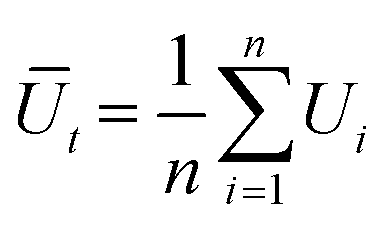 | (6) |
 | (7) |
Additionally, the mean particle number per frame d at global red illumination only (time interval 0 s to 5 s) and with additional local illumination (time interval 10s to 45 s) i, are computed. The particle numbers are averaged using the arithmetic mean of the particle number per frame ni for all frames m in the corresponding time interval.
 | (8) |
Data availability
The data supporting this article have been included as part of the ESI.† Primary data (uploaded video files) supporting this article have been included as part of the ESI† uploaded on publisher website.Author contributions
M. B. and F. R. concepted the work and wrote the manuscript. F. R. performed all data analysis and data treatment. D. V. M., I. M. performed supporting measurements and data analysis. N. L. synthesized the surfactant. S. S. helped supervise the project and aided in interpreting the results.Conflicts of interest
The authors declare no conflict of interest.Acknowledgements
M. B. gratefully acknowledges financial support by the German Research Foundation (DFG) through the grant BE 7745/1-1 (project number 469240574).Notes and references
- B. V. Derjaguin, G. Sidorenkov, E. Zubashchenko and E. Kiseleva, Prog. Surf. Sci., 1993, 43, 138–152 CrossRef
.
- J. L. Anderson, Annu. Rev. Fluid Mech., 1989, 21, 61–99 CrossRef
- A. Domínguez and M. N. Popescu, Curr. Opin. Colloid Interface Sci., 2022, 61, 101610 CrossRef
- B. Abécassis, C. Cottin-Bizonne, C. Ybert, A. Ajdari and L. Bocquet, Nat. Mater., 2008, 7, 785–789 CrossRef PubMed
- S. Marbach and L. Bocquet, Chem. Soc. Rev., 2019, 48(11), 3102–3144 RSC
- S. Battat, J. T. Ault, S. Shin, S. Khodaparast and H. A. Stone, Soft Matter, 2019, 15, 3879–3885 RSC
- T. Tsuji, Y. Sasai and S. Kawano, Phys. Rev. Appl., 2018, 10, 044005 CrossRef CAS
- J. Palacci, B. Abécassis, C. Cottin-Bizonne, C. Ybert and L. Bocquet, Phys. Rev. Lett., 2010, 104, 138302 CrossRef PubMed
- C. Lee, C. Cottin-Bizonne, A.-L. Biance, P. Joseph, L. Bocquet and C. Ybert, Phys. Rev. Lett., 2014, 112, 244501 CrossRef CAS PubMed
- S. Shin, E. Um, B. Sabass, J. T. Ault, M. Rahimi, P. B. Warren and H. A. Stone, Appl. Phys. Sci., 2015, 113, 257–261 Search PubMed
- S. Shin, Phys. Fluids, 2020, 32, 101302 CrossRef CAS
- S. Shim, Chem. Rev., 2022, 122(7), 6986–7009 CrossRef CAS PubMed
- N. Shi, R. Nery-Azevedo, A. I. Abdel-Fattah and T. M. Squires, Phys. Rev. Lett., 2016, 117(25), 258001 CrossRef PubMed
- A. Persat, R. Chambers and J. Santiago, Lab Chip, 2009, 9, 2437–2453 RSC
- A. Persat, M. Suss and J. Santiago, Lab Chip, 2009, 9, 2454–2469 RSC
- V. Doan, P. Saingam, T. Yan and S. Shin, ACS Nano, 2020, 14, 14219–14227 CrossRef CAS PubMed
- A. Banerjee, I. Williams, R. N. Azevedo, M. E. Helgeson and T. M. Squires, Proc. Natl. Acad. Sci. U. S. A., 2016, 113, 8612–8617 CrossRef CAS PubMed
- R. Nery-Azevedo, A. Banerjee and T. Squires, Langmuir, 2017, 33, 9694–9702 CrossRef CAS PubMed
- S. Shin, P. Warren and H. Stone, Phys. Rev. Appl., 2018, 9, 034012 CrossRef CAS
- A. Banerjee, H. Tan and T. Squires, Phys. Rev. Fluids, 2020, 5, 073701 CrossRef
- S. Shim, S. Khodaparast, C.-Y. Lai, J. Yan, J. T. Ault, B. Rallabandi, O. Shardt and H. A. Stone, Soft Matter, 2021, 17, 2568–2576 RSC
- S. Shin, O. Shardt, P. Warren and H. Stone, Nat. Commun., 2017, 8, 1 CrossRef CAS PubMed
- S. Shim, M. Baskaran, E. Thai and H. Stone, Lab Chip, 2021, 21, 3387–3400 RSC
- S. Shim and H. Stone, Proc. Natl. Acad. Sci. U. S. A., 2020, 117, 25985–25990 CrossRef CAS PubMed
- T. J. Shimokusu, V. G. Maybruck, J. T. Ault and S. Shin, Langmuir, 2020, 36, 7032–7038 CrossRef CAS PubMed
- B. Abécassis, C. Cottin-Bizonne, C. Ybert, A. Ajdari and L. Bocquet, Nat. Mater., 2008, 7, 785–789 CrossRef PubMed
- J. S. Paustian, R. N. Azevedo, S.-T. B. Lundin, M. J. Gilkey and T. M. Squires, Phys. Rev. X, 2013, 3, 041010 CAS
- C. Lee, C. Cottin-Bizonne, A.-L. Biance, P. Joseph, L. Bocquet and C. Ybert, Phys. Rev. Lett., 2014, 112, 244501 CrossRef CAS PubMed
- A. Kar, T.-Y. Chiang, I. Ortiz-Rivera, A. Sen and D. Velegol, ACS Nano, 2015, 9, 746–753 CrossRef CAS PubMed
- A. Banerjee, I. Williams, R. N. Azevedo, M. E. Helgeson and T. M. Squires, Proc. Natl. Acad. Sci. U. S. A., 2016, 113, 8612–8617 CrossRef CAS PubMed
- M. Bekir, M. Sperling, D. V. Muñoz, C. Braksch, A. Böker, N. Lomadze, M. N. Popescu and S. Santer, Adv. Mater., 2023, 35, 2300358 CrossRef CAS PubMed
- D. Vasquez-Muñoz, F. Rohne, A. Sharma, N. Lomadze, S. Santer and M. Bekir, Small, 2024, 2401144 CrossRef PubMed
- D. Feldmann, P. Arya, T. Y. Molotilin, N. Lomadze, A. Kopyshev, O. I. Vinogradova and S. Santer, Langmuir, 2020, 36, 6994 CrossRef CAS PubMed
- A. Sharma, M. Bekir, N. Lomadze, S.-H. Jung, A. Pich and S. Santer, Langmuir, 2022, 38, 6343–6351 CrossRef CAS PubMed
- P. Arya, M. Umlandt, J. Jelken, D. Feldmann, N. Lomadze, E. S. Asmolov, O. I. Vinogradova and S. A. Santer, Eur. Phys. J. E:Soft Matter Biol. Phys., 2021, 44(50), 1–10 Search PubMed
- J. Eastoe and A. Vesperinas, Soft Matter, 2005, 1, 338 RSC
- Y. Zakrevskyy, J. Roxlau, G. Brezesinski, N. Lomadze and S. Santer, J. Chem. Phys., 2014, 140, 044906 CrossRef PubMed
- P. Arya, J. Jelken, N. Lomadze, S. Santer and M. Bekir, J. Chem. Phys., 2020, 152, 024904 CrossRef CAS PubMed
- M. Montagna and O. Guskova, Langmuir, 2018, 34, 311 CrossRef CAS PubMed
- S. Santer, J. Phys. D: Appl. Phys., 2018, 51, 013002 CrossRef
- A. Sharma, S.-H. Jung, N. Lomadze, A. Pich, S. Santer and M. Bekir, Macromolecules, 2021, 54, 10682 CrossRef CAS
- M. Bekir, A. Sharma, M. Umlandt, N. Lomadze and S. Santer, Adv. Mater. Interfaces, 2022, 9, 2102395 CrossRef CAS
- D. Feldmann, P. Arya, N. Lomadze, A. Kopyshev and S. Santer, Appl. Phys. Lett., 2019, 115, 263701, DOI:10.1063/1.5129238
- A. J. Goldman, R. G. Cox and H. Brenner, Chem. Eng. Sci., 1967, 22, 653 CrossRef CAS
- R. Brandão, G. G. Peng, D. Saintillan and E. Yariv, Phys. Rev. Fluids, 2024, 9, 014001 CrossRef
- A. M. J. Davis and E. Yariv, J. Eng. Math., 2022, 133, 5 CrossRef CAS
- M. Umlandt, D. Feldmann, E. Schneck, S. Santer and M. Bekir, Langmuir, 2020, 36, 14009 CrossRef CAS PubMed
- D. Vasquez Muñoz, F. Rohne, I. Meier, A. Sharma, N. Lomadze, S. Santer and M. Bekir, Small, 2024, 43, 202403546 Search PubMed
Footnote |
| † Electronic supplementary information (ESI) available. See DOI: https://doi.org/10.1039/d4lc01092b |
| This journal is © The Royal Society of Chemistry 2025 |