
 Open Access Article
 This Open Access Article is licensed under a Creative Commons Attribution-Non Commercial 3.0 Unported Licence
Toxicokinetics for organ-on-chip devices†
Nathaniel G.
Hermann
 a,
Richard A.
Ficek
a,
Dmitry A.
Markov
b,
Lisa J.
McCawley
b and
M. Shane
Hutson
*a
a,
Richard A.
Ficek
a,
Dmitry A.
Markov
b,
Lisa J.
McCawley
b and
M. Shane
Hutson
*a
aDepartment of Physics and Astronomy, Vanderbilt University, PMB 401807, Nashville, TN 37240, USA. E-mail: shane.hutson@vanderbilt.edu
bDepartment of Biomedical Engineering, Vanderbilt University, USA
First published on 10th March 2025
Abstract
Organ-on-chip (OOC) devices are an emerging New Approach Method in both pharmacology and toxicology. Such devices use heterotypic combinations of human cells in a micro-fabricated device to mimic in vivo conditions and better predict organ-specific toxicological responses in humans. One drawback of these devices is that they are often made from polydimethylsiloxane (PDMS), a polymer known to interact with hydrophobic chemicals. Due to this interaction, the actual dose experienced by cells inside OOC devices can differ strongly from the nominal dose. To account for these effects, we have developed a comprehensive model to characterize chemical–PDMS interactions, including partitioning into and diffusion through PDMS. We use these methods to characterize PDMS interactions for 24 chemicals, ranging from fluorescent dyes to persistent organic pollutants to organophosphate pesticides. We further show that these methods return physical interaction parameters that can be used to accurately predict time-dependent doses under continuous-flow conditions, as would be present in an OOC device. These results demonstrate the validity of the methods and model across geometries and flow rates.
Introduction
Organ-on-chip (OOC) devices are a promising new approach method for pharmacology and toxicology in which human cells are cultured under microfluidic perfusion. Such devices can reproduce human organ responses at a miniaturized scale and thus have advantages over animal testing in terms of cost, ethical concerns, and adaptability for high-throughput screening;1–7 however, their small channel sizes yield large surface-area-to-volume ratios, which exacerbate losses resulting from chemicals interacting with the materials of the channel walls. One key material used to fabricate OOC devices is the elastomer polydimethylsiloxane (PDMS). This material is transparent, flexible, biocompatible and relatively low cost, which makes it ideal for prototyping OOC devices in academic labs. As market demand for OOC devices has grown,8 PDMS remains the bulk material in many commercially available devices, e.g., those sold by Emulate9 and SynVivo.10–13 Other commercial OOC suppliers have moved away from PDMS in favor of injection-molded thermoplastics (ChipShop)14,15 or glass (Micronit),16 but even in these devices, PDMS or another soft polymer is often incorporated to make flexible membranes and valves. Unfortunately, the use of PDMS in microfluidic devices has a well-recognized drawback: PDMS tends to interact with and sequester hydrophobic compounds.17–24 When that happens, a compound's nominal inlet concentration is no longer a reliable measure of its in-device chemical dose.There are three strategies for dealing with this problem: (1) avoid testing of hydrophobic chemicals; (2) mitigate the interactions by modifying PDMS, by including a carrier in solution, or by using a different elastomeric material; or (3) measure and model the interactions to account for them and predict time-dependent in vitro concentration profiles within such devices. Here, we take the latter toxicokinetic approach. We demonstrate relatively simple methods for measuring the chemical–PDMS interaction parameters that govern partitioning at water–PDMS interfaces and diffusion in PDMS bulk. We measure these parameters for 24 compounds and find that their values vary across several orders of magnitude. Importantly, these microscopic parameters are independent of geometry and flow rate, which makes the associated model extensible to any user-defined geometry. We validate this independence and extensibility by demonstrating the ability of a 3D finite-element model to use the parameters measured in static disk-soak and diffusion-through-membrane experiments to accurately predict concentration profiles in microfluidic channels at two different flow rates. These methods and models are one key step in the larger task of translating in vitro dose to equivalent in vivo organal dose, i.e., in vitro–in vivo extrapolation (IVIVE).7,25
We have pursued this modeling approach because the other two strategies are not always feasible. In some cases, one can avoid testing hydrophobic chemicals, but that strategy is unworkable for many applications in environmental toxicology: high hydrophobicity is a key characteristic of many persistent organic pollutants. For this study, we selected several such compounds: three organophosphate pesticides or pesticide metabolites – chlorpyrifos, paraoxon, and parathion – that have been the subject of prior studies with an organ-on-chip neurovascular unit26 or microphysiometer;27,28 a polycyclic aromatic hydrocarbon, benzo[a]pyrene, previously studied both for its ability to disrupt endocrine signaling in an endometrium-on-a-chip device29,30 and as a component of cigarette smoke extract (CSE) studied in a fetal membrane-organ-on-chip;31 and a pharmaceutical, amodiaquine, that has been studied in a human-airway-on-a-chip.32,33 We complemented this set of toxicants and drugs with four fluorescent dyes – fluorescein, fluorescein-5-isothiocyanate (FITC), rhodamine B, rhodamine 6G – that have been used in several studies as tracers and/or analogs for PDMS interactions.33–35 Finally, we included indole, which is fairly water soluble (3.56 mg mL−1), relatively non-toxic, and serves as an excellent control that interacts with PDMS quickly, but not prohibitively strongly. As shown in Table 1, each of these ten chemicals has an octanol–water coefficient above the log![[thin space (1/6-em)]](https://www.rsc.org/images/entities/char_2009.gif) P = 1.8 threshold where interactions with PDMS become a concern.22
P = 1.8 threshold where interactions with PDMS become a concern.22
P sourced from PubChem36
| Chemical | logP |
logKPW |
logKPD |
logDP (mm2 h−1) |
logDS (mm2 h−1) |
logH (mm h−1) |
|---|---|---|---|---|---|---|
| Rhodamine 6G | 6.4 | — | — | — | — | — |
| Benzo[a]pyrene | 6.1 | 5.20 ± 1.22 | −2.06 ± 0.82 | −1.42 ± 0.30 | −1.89 ± 0.26 | −0.49 ± 0.17 |
| Chlorpyrifos | 5.0 | 6.25 ± 1.98 | −1.21 ± 0.53 | −1.51 ± 0.30 | ≥3.56 | 0.04 ± 0.09 |
| FITC | 4.8 | — | — | — | — | — |
| Parathion | 3.8 | 4.39 ± 0.50 | −1.92 ± 0.47 | −1.40 ± 0.50 | ≥3.56 | −1.05 ± 0.14 |
| Amodiaquine | 3.7 | −0.84 ± 0.63 | — | −1.29 ± 0.58 | ≥3.56 | ≥1.56 |
| Fluorescein | 3.4 | — | — | — | — | — |
| Indole | 2.1 | −0.91 ± 0.03 | −1.12 ± 0.26 | −1.25 ± 0.09 | 0.56 ± 0.07 | ≥1.56 |
| Paraoxon | 2.0 | 1.08 ± 0.03 | — | −1.96 ± 0.05 | 0.52 ± 0.23 | ≥1.56 |
| Rhodamine B | 1.9 | 1.83 ± 0.10 | — | −3.44 ± 0.68 | −1.16 ± 0.12 | ≥1.56 |
As for mitigation strategies, several groups are working on alternative materials,37,38 but PDMS has many properties – low cost, flexibility, transparency, gas permeability, and biocompatibility – that make it ideal for microfabricating OOC devices;6,23 it thus remains the dominant OOC material. Researchers have also evaluated mitigation techniques that modify PDMS surfaces to somewhat limit chemical–PDMS interactions. One popular approach is plasma oxidation, which makes PDMS surfaces hydrophilic and eliminates interactions with hydrophobic chemicals. Unfortunately, this change is transient: PDMS will revert to an intermediate value of hydrophobicity at a rate that depends on the degree of initial oxidation and subsequent storage conditions.39–41 This partial, time-dependent reversion only complicates attempts to account for and model interactions with hydrophobic compounds. Finally, many researchers include serum, purified serum transport proteins, or micelle-forming detergents to serve as carriers in the culture medium. If any of these are present in sufficient quantities, they can stabilize the free concentrations of hydrophobic compounds.42,43 Nonetheless, some applications require the use of serum-free or detergent-free media. Even when carriers can be added, determining whether the free concentrations are stabilized, and at what levels, requires modeling approaches with additional parameters, complicating the picture.
Given the above limitations of mitigation, we proffer mass transport modeling as a ubiquitously applicable tool to account for chemical–PDMS interactions within OOC devices. This approach requires measurements of the microscopic PDMS interaction parameters for a given chemical, but the needed experiments are within the means of the typical laboratory. Even without experiments, the parameters can be estimated using quantitative structure–property relation (QSPR) models.44,45 One can then use finite-element modeling (FEM) to simulate a specific device, flow rate, and time-dependent inlet concentration to determine dynamic in-device concentration profiles.
Methods
PDMS preperation
PDMS Sylgard 184 (Dow Corning, Auburn, MI) was mixed in a 10:1 mass ratio of elastomer base to curing agent. To make PDMS disks, PDMS was cast in a 6 mm thick layer, which was then cured overnight in a 67 °C oven. After curing, disks were prepared with a 3 mm radius biopsy punch. These PDMS disks were then annealed for 4 hours in a 200 °C oven to stabilize mechanical properties.46 PDMS membranes were spun out from small volumes of PDMS to 80 μm thickness on a Laurell WS-400-6NPP Spin Coater (Laurell Technologies Corporation, Lansdale, PA) using the procedure described by Markov et al.41 and then cured. PDMS with microchannels, measuring 21.1 mm in length, 1.5 mm in width, and 100 μm in height, was made by casting 6 mm of PDMS over a SU-8 photoresist mold. The cast PDMS was then allowed to cure, and annealed. For experiments, each block of PDMS with microchannels was clamped onto a 2 inch by 3 inch microscope slide.
Chemical preparation
Chemicals were acquired either as powders or liquids from Sigma Aldrich (St. Louis, MO). Stock solutions were prepared with 1× pH-7.4 phosphate buffered saline (PBS) (Thermo Fisher, Waltham, MA) to near maximum solubility. For chemicals with very low solubility in water, dimethyl sulfoxide (DMSO) was added to increase solubility. DMSO does not partition into nor interact with PDMS, making it a compatible organic solvent.47 For experiments, stock solutions were diluted in their respective mixed solvent to obtain a peak UV-vis absorbance close to one. The concentrations used in experiments were in the micromolar range (Table S1†).Measuring chemical loss to PDMS in disk-soak experiments
Disk-soak experiments were performed by monitoring loss of chemical from solution over time while in contact with a PDMS disk. Concentrations were estimated via UV-vis absorbance spectra measured with a NanoDrop OneC UV-vis spectrophotometer (Thermo Fisher, Waltham, MA).Disk soak experiments were conducted with 2 mL of chemical solution in type 1P disposable UV plastic cuvettes (FireflySci, Northport, NY). Disks were gently placed on top of this solution such that they floated with only the top surface above the solution (Fig. 1A). Cuvettes were sealed with tight fitting PFTE covers to prevent evaporation. These cuvettes had spectra measured in the spectrophotometer at pseudo-logarithmic times over 48 hours to record concentration loss, while the remainder of the time they were left on a blot mixer to ensure solutions remained well mixed. Simultaneously, a cuvette of solution with no disk was monitored to control for any chemical interaction with UV plastic. After 48 hours, disks were removed, dried, and placed in cuvettes filled with fresh solvent. These cuvettes were then sealed and monitored for 48 hours to track chemical release from PDMS.
 | ||
| Fig. 1 Experimental setups. (A-left) Schematic of a disk-soak experiment in which a disk of PDMS is floated in a cuvette containing a chemical solution of interest; (A-right) an example pre-equilibrium profile of chemical concentration in the solution and PDMS disk. (B-left) Schematic of a membrane experiment in which a thin PDMS membrane separates a source chamber loaded with a chemical solution of interest and a sink chamber loaded with matching solvent; (B-right) an example pre-equilibrium profile of chemical concentration in source chamber, PDMS membrane, and sink chamber. | ||
Measuring chemical diffusion through PDMS
Diffusion-through-membrane experiments were carried out in aluminum devices fabricated in-house. Each device had source and sink reservoirs that were separated by an 80 μm thick PDMS membrane. To prevent leaks, the PDMS–aluminum interface was sealed with high vacuum grease (Dow Corning, Midland, MI). The source and sink were loaded with 200 μL of either chemical solution or matching solvent, respectively. A piece of Scotch tape was used to seal the top of the reservoirs to prevent evaporation (Fig. 1B). For chemicals with reasonable solubility and strong UV/vis absorbance, concentrations for the source and sink were measured from UV-vis absorbance spectra of 2 μL aliquots using the attenuated total reflectance pedestal of the NanoDrop OneC spectrophotometer. For chemicals with weaker absorbance, the full 200 μL was removed from each chamber, placed in a cuvette for measurement of its UV-vis absorbance spectrum, and then returned to its original chamber. For most chemicals, measurements were taken at pseudologarithmic intervals over 24 hours. For those chemicals that exhibited fast diffusion, measurements were then repeated at ten minute intervals over 1 hour.Direct optical measurement of diffusion in PDMS
For select fluorescent dyes, diffusion in PDMS was also assayed via direct optical visualization. To do so, a 21.1 mm long by 1.5 mm wide by 100 μm tall microchannel in PDMS was filled with a solution of a fluorescent dye, and imaged for three hours using a 1× objective on a Nikon Ti2 Eclipse with X-light V2 spinning disk confocal microscope (Nikon Instruments, Melville, NY). After this time, the microchannel was emptied and dried. The walls of the dry channel were then imaged for an additional 12 hours to follow the diffusive spread of any dye that had previously partitioned into the PDMS. The spatial profile of diffusing dye was fit to a solution to the 1D diffusion equation to estimate diffusivity in PDMS, DP.Measuring chemical loss under constant pumped flow
To replicate chemical loss in a continually perfused PDMS device, we measured chemical loss to PDMS in microchannels perfused at constant flow rates of 5 or 10 μL min−1. Perfusion was controlled by a Hamilton Standard Infuse/Withdraw Pump 11 Pico Plus Elite Programmable syringe pump (Harvard Apparatus, Hollison, MA) with 2.5 mL Hamilton syringes (Hamilton, Reno, NV) coupled to the microchannels using Tefzel tubing (McMaster-Carr, Elmhurst, IL). Effluent was collected in 10 min intervals and chemical concentration in each effluent sample was measured via UV-vis absorbance using the pedestal of the NanoDrop OneC spectrometer.Simulating experiments and fitting experimental data
Disk-soak, membrane and pumped-flow experiments were simulated using the finite element modeling (FEM) software COMSOL Multiphysics (COMSOL, Inc., Burlington, MA). Disk-soak and pumped-flow experiments were simulated in full three dimensions; simulations of membrane experiments could be reduced by symmetry to just one dimension.Data from disk-soak and membrane experiments were fit to results from the FEM simulations to estimate chemical-specific model parameters. To make these estimates, simulations of both experiments were run across a uniformly log-spaced grid of all model parameters. This set of 4802 simulations was used to construct a first-order interpolation function, and the experimental concentration data were then fit to this function. Construction of the interpolation function and its regression against experimental data was performed in Mathematica (Wolfram, Champagne, IL).
Results
We tested ten hydrophobic chemicals (logP ≥ 1.9) with both disk-soak and membrane experiments to measure each chemical's interactions with PDMS. Seven of these chemicals were sufficiently water-soluble to make measurements directly in phosphate-buffered saline (Fig. 2 and S1†). An additional three were insufficiently water-soluble and required the addition of ≥40% DMSO by volume (Fig. 3A). These chemical's interactions were remarkably varied: some did not partition into PDMS at any detectable level (e.g., FITC in Fig. 2), but others partitioned very strongly, depleting the concentration in solution by up to 80% (e.g., parathion in Fig. 3A); with similarly wide variation, some chemicals diffused through an 80 μm thick PDMS membrane as fast as 1–5 h (e.g., indole and paraoxon in Fig. 2), while others needed 12–24 h or longer (e.g., amodiaquine and rhodamine B in Fig. 2), and at least one bound to PDMS surfaces, but did not diffuse into the PDMS bulk (rhodamine 6G, Fig. S3†). Note that many of the membrane experiments reached final equilibria in which the sum of the source and sink concentrations was less than the initial concentration, revealing that a substantial fraction of the chemical remained in the thin PDMS membrane (e.g., parathion and benzo[a]pyrene in Fig. 3A).
 | ||
| Fig. 2 Disk-soak and membrane experiment results for chemicals in solutions of PBS. Left column shows disk-soak data and associated fits (dashed). Right column shows membrane data from both source (filled) and sink (empty) with associated fits (dashed). Since FITC demonstrates no interaction, no fit is shown. | ||
 | ||
| Fig. 3 Disk-soak and membrane experiment results for chemicals with added DMSO cosolvent. (A – left column) Disk-soak data for each chemical in mixed solvents at three different DMSO volume fractions, color-coded to match the three right columns with blue, green, and red running from low to high DMSO fraction. (A – right columns) Source and sink data (closed and open symbols) from membrane experiments for each chemical at the noted DMSO volume fraction. Fits shown as dashed lines. (B) Best-fit values of logK versus DMSO volume fraction and linear fits (dashed lines) used to extrapolate to the PDMS–water partition coefficients, logKPW. (C) Best-fit values of logDPversus DMSO volume fraction. Legend in B applies to B and C. | ||
Parameterizing and modeling chemical–PDMS interactions
To be more broadly useful, measurements of chemical–PDMS interactions must be parameterized with a model that can be extended to other PDMS geometries and solution flow rates. In prior work, we parameterized chemical–PDMS interactions with a surface binding model, which fit disk-soak data well,22 but did so only for unrealistically large surface binding capacities. This shortcoming strongly suggests that chemicals diffuse away from the surface and into the PDMS bulk, leading the model to make inaccurate predictions when this diffusion becomes important – e.g., at long times when a solution of interest is flowing through microchannels in a large volumetric excess of PDMS.To parameterize chemical–PDMS interactions in a more accurate and physically realistic manner, we use a model that includes both partitioning at solution–PDMS interfaces and diffusion through bulk PDMS. This model uses two linked variables to describe the concentration of a given chemical species in solution, cS, and in PDMS, cP. The concentrations evolve over time as described by the following partial differential equations
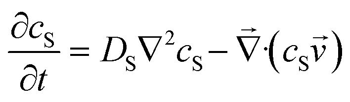 | (1) |
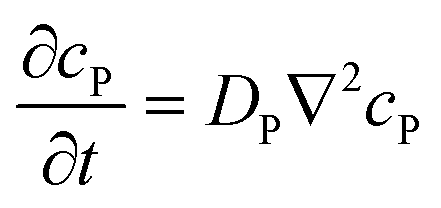 | (2) |
 | (3) |
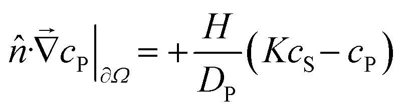 | (4) |
![[v with combining right harpoon above (vector)]](https://www.rsc.org/images/entities/i_char_0076_20d1.gif) (t; x, y, z) defines local flow rates in the aqueous solution. These partial differential equations can be solved numerically for any flow rate field and user-defined solution–PDMS geometry.‡ The model is applicable as long as its parameters remain concentration independent. We have observed break downs of the model at high concentrations when the surface layers of PDMS become saturated with chemical; under those conditions, the apparent partition coefficient decreases with increasing cS.
(t; x, y, z) defines local flow rates in the aqueous solution. These partial differential equations can be solved numerically for any flow rate field and user-defined solution–PDMS geometry.‡ The model is applicable as long as its parameters remain concentration independent. We have observed break downs of the model at high concentrations when the surface layers of PDMS become saturated with chemical; under those conditions, the apparent partition coefficient decreases with increasing cS.
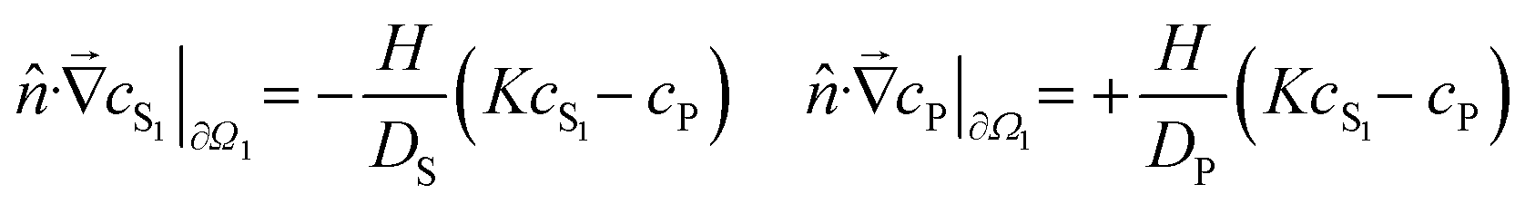
In the case of membrane experiments, we extend the model to consider concentrations in both the source and sink chambers. The equations remain similar, but with two solution concentrations, cS1 and cS2, representing the source and sink respectively:


To fit this model to our experimental data, we first used COMSOL Multiphysics to run a large set of finite-element simulations based on the geometries of disk-soak and membrane experiments and covering 4802 different parameter combinations. These simulations were performed over a log-scaled grid of the four parameters: logDS from −2.44 to 3.56 (DS in units of mm2 h−1); logDP from −6.44 to −0.44 (DP in units of mm2 h−1); logH from −4.44 to 1.56 (H in units of mm h−1); and logK from −2.00 to 4.00. The numeric model outputs were then used to construct first-order interpolation functions for the average concentration in solution as a function of time and model parameters, cSi(DS, DP, H, K, t), where the subscript i denotes applicability to either disk-soak or membrane experiments. The interpolation functions were then regressed against experimental data to estimate the best-fit parameters for each chemical–solvent combination. The most tightly constrained parameter estimates were obtained by fitting both disk-soak and membrane data simultaneously using shared parameters. When data from disk-soak experiments was fit separately, regression yielded reasonably constraints for the product  , but not for the individual parameters K and DP. The simultaneous fits relieved this degeneracy.
Of the seven sufficiently water-soluble chemicals tested here, four partitioned into and diffused through PDMS. The data and fits for these four chemicals are shown in Fig. 2, with the best-fit parameters compiled in Table 1. Three of the four (rhodamine B, paraoxon, and indole) partitioned favorably into PDMS (KPW ≈ 68, 12 and 8.1, respectively), while amodiaquine partitioned quite weakly (KPW ≈ 0.14). A different set of three (indole, paraoxon, and amodiaquine) diffused through PDMS at similar rates with DP = 0.01 to 0.06 mm2 h−1, while rhodamine B diffused much slower (4 × 10⁻⁴ mm2 h−1). Note that even the fast-diffusing chemicals have diffusion constants in PDMS that are two orders of magnitude slower than those in water.
Modification of chemical–PDMS interactions by cosolvent
When a chemical of interest is poorly soluble and not spectroscopically detectable in pure PBS, its solubility can be increased by adding a cosolvent such as DMSO; however, adding cosolvent also affects the partitioning of a chemical between the now mixed solvent and PDMS. We thus explored whether this effect can be accounted for using an extension of the log-linear solubility model of Yalkowsky:51| logSm = (1 − f)logSw + flogSc | (5) |
| logKAB = logSA − logSB |
| logKPM = (1 − f)logKPW + flogKPC | (6) |
KPM should thus be a linear function of the cosolvent fraction. Given that this model is derived from Yalkowsky's log-linear model, we expect it to perform well for classes of chemicals described well by the original model, which assumes an ideal, non-volatile solution.
To test the validity of the log-linear model, we conducted disk-soak and membrane experiments for indole at four DMSO volume fractions from 10% to 70% (Fig. 3A and B). The plot of logKPMversus f appears linear, and the extrapolation back to 0% DMSO yields logKPW = 0.76 ± 0.14. The agreement between this extrapolated value and that measured directly in pure PBS, 0.91 ± 0.03, confirms the applicability of the log-linear model.
We then conducted disk-soak and membrane experiments across a range of DMSO fractions for three poorly soluble compounds—benzo[a]pyrene, chlorpyrifos, and parathion (Fig. 3A). We fit the data in each mixed solvent to the partition–diffusion model, and used the log-linear model to estimate the partition coefficient expected in pure PBS (Fig. 3B). With the caveat that the log-linear model likely only provides an order-of-magnitude estimate of logKPW, we used it to extrapolate the PDMS–water partition coefficient for each of the poorly soluble chemicals (Fig. 3B), and present these values as logKPW in Table 1. For each of the poorly water-soluble chemicals, the PDMS–water partition coefficients were estimated to be in the range of 400 to 2000, which is one to two orders of magnitude greater than those of the water-soluble chemicals. The corresponding estimates in pure DMSO, logKPD = logKPC, are also presented in Table 1 to allow interpolation to any DMSO fraction.
To estimate the other model parameters, we simply report the mean of their values obtained at various cosolvent fractions (Table 1). This approach seems very reasonable for diffusivity in PDMS, DP, which should be independent of any cosolvent present in the solution phase. Consistent with this expectation, estimates ofDP in different mixed solvents do not show any clear trend with DMSO fraction (Fig. 3C). The average value of DP for these chemicals is fairly consistent, around 0.035 mm2 h−1. As shown in Fig. 4, the extrapolation for chemicals tested in high DMSO fraction places looser constraints on logDP and logK than direct tests in aqueous solution.
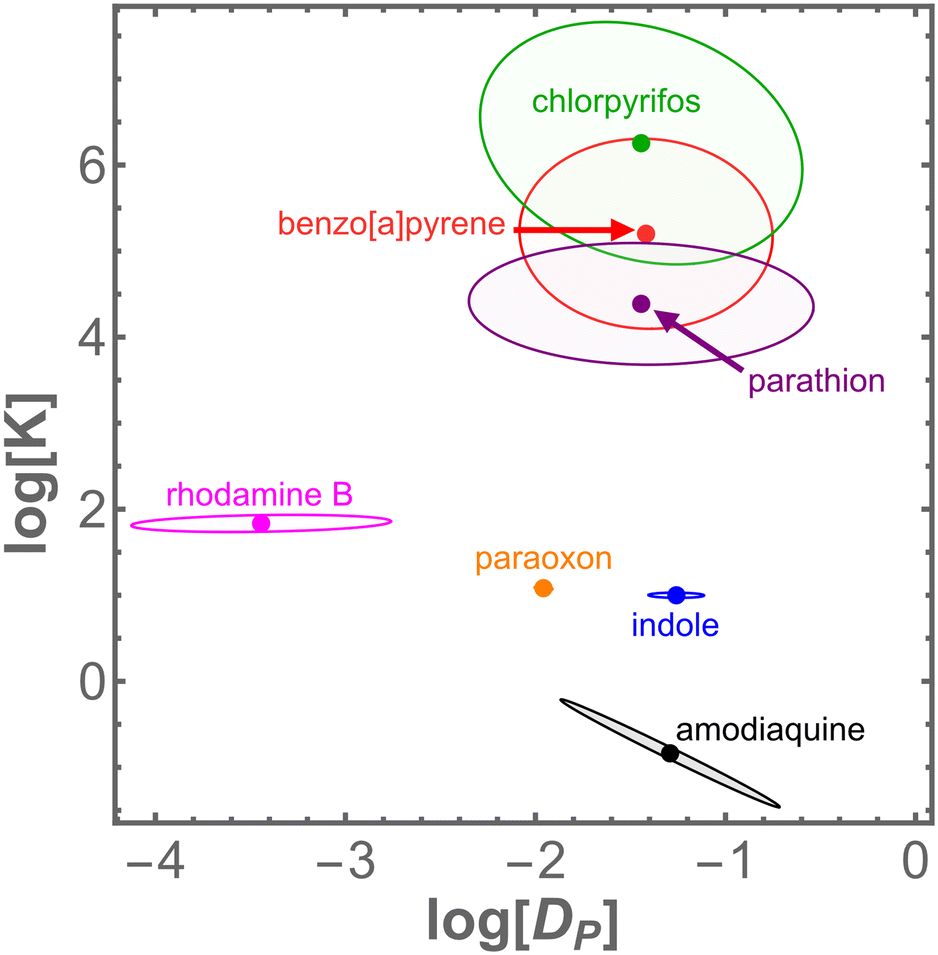 | ||
| Fig. 4 Fitted values of logDP and logKPW with corresponding error ellipses for four chemicals measured directly in aqueous solutions (amodiaquine, indole, paratoxon, rhodamine B) and three measured in solutions with DMSO (benzo[a]pyrene, chlorpyrifos, and parathion). | ||
As for the diffusivity in solution, DS, one might expect a dependence on cosolvent. As has been shown by Miyamoto and Shimono, the diffusivity in a solvent of small hydrophobic molecules can be well modeled by the Stokes–Einstein equation

Direct imaging of diffusion in PDMS
To validate the estimates of DP obtained from fits to the 3D partition–diffusion model, we directly imaged the diffusion of fluorescent dyes into bulk PDMS. If a dye is distributed with an initial 1D fluorescence profile u(x, 0) that is well approximated by a Gaussian of 1/e2-width σ0, then its subsequent time-dependent profile under Fickian diffusion with no-flux boundary conditions is given by | (7) |
| σ(t)2 = 2DPt + σ02 | (8) |
To match these conditions, we loaded microchannels with dye solutions, allowed the dye to diffuse into the channels' PDMS walls for three hours, emptied the microchannels, and then imaged the diffusive spread of preloaded dye further into the PDMS bulk – without the complicating effects of further partitioning. For each dye, at each time t, we fit the fluorescence intensity profile to eqn (7) to estimate the Gaussian square width, σ2. We then used a linear fit of σ2(t) to eqn (8) to estimate DP. Among the four dyes in our test set, only rhodamine B and 6G bind to or partition into PDMS. We directly imaged the diffusion of both. Rhodamine 6G does not measurably diffuse beyond the PDMS surface, but rhodamine B clearly does, spreading from a width of ∼50 μm to ∼150 μm over 12 h (Fig. 5A and B and S7†). When measured in this direct manner, we estimate the diffusion constant of rhodamine B in PDMS as logDP = −3.907 ± 0.004 (in mm2 h−1; Fig. 5C), which agrees with the best-fit value found indirectly via disk-soak and membrane experiments, logDP = −3.44 ± 0.68. In similar agreement, the inability of rhodamine 6G to diffuse further into PDMS matches its inability to diffuse through a thin PDMS membrane (Fig. S1†).
 | ||
| Fig. 5 Direct imaging of fluorescent dye diffusion into bulk PDMS. (A) The fluorescence intensity profile of rhodamine B spreads diffusively into PDMS over 12 h. (B) In contrast, the fluorescence intensity profile of rhodamine 6G is essentially static over 12 h, indicating a lack of diffusion into PDMS. (C) For rhodamine B, the Gaussian square width, σ, grows linearly, with linear regression yielding a best-fit value of DP (as labeled, in units of mm2 h−1) that agrees with that found indirectly in Table 2. For rhodamine 6G, the Gaussian square width does not measurably change with time. | ||
Loss of indole during continuous flow in microchannels
To illustrate the applicability of the 3D partition–diffusion model across geometries and flow rates, we used COMSOL Multiphysics to simulate continuous pumped flow of an indole solution through rectangular PDMS channels and compared the results with data from matching experiments. In this case, the parameters for indole were obtained from disk-soak and membrane experiments (Table 2) and used without modification to directly simulate the first three hours of continuous flow of indole through microchannels at two flow rates, Q = 5 and 10 μL min−1. These microchannels were originally used as a microfluidic supply network for cell chambers in a thick tissue bioreactor.34 As shown in Fig. 6A and S7,† the partitioning and diffusion of indole into PDMS creates two gradients within the device—one longitudinal along the flow direction and one perpendicular to it. The stronger perpendicular gradient is readily apparent in Fig. 6A. We imaged similar gradients of fluorescent dyes in statically filled channels in Fig. 5, but we cannot directly image the indole gradient inside the device. The longitudinal gradient is more subtle but readily measurable. As shown in Fig. 6B, this gradient is time-dependent: at the earliest time point, the indole concentration decreases by approximately 60% over the length of the channel, but this drop becomes shallower over time. We cannot sample the concentration along the length of the channel due to limitations on experimental sampling volume: the microchannel only contains 3.2 μL of fluid. Instead, since the inlet concentration is fixed, we can compare the model's predicted gradients against experiments by measuring the concentration at the channel outlet (i.e., at z = 21.1 mm). In these matching experiments, an indole solution was pumped through a microchannel at the same flow rates, and effluent was collected in bins across the duration of the experiment. For the higher flow rate, the simulations slightly underestimate the experimental outlet concentrations in the first hour, but are a good match at longer times; for the lower flow rate, the simulations and experiments are a good match at all times (Fig. 6C). This agreement illustrates the physicality and wide applicability of the model and the methods presented here for inferring its chemical-specific model parameters.| Chemical | logKPW |
logDP (mm2 h−1) |
logDS (mm2 h−1) |
logH (mm h−1) |
|---|---|---|---|---|
| Ethofumesate | 1.48 ± 0.03 | −1.67 ± 0.08 | ≥3.56 | ≥1.56 |
| Acridine orange | 1.28 ± 0.04 | −4.29 ± 0.09 | ≥3.56 | −1.54 ± 0.16 |
| Diacetone alcohol | 1.20 ± 0.02 | −1.77 ± 0.33 | ≥3.56 | −0.81 ± 0.16 |
| Cyclohexanol | 0.75 ± 0.19 | −1.77 ± 0.20 | ≥3.56 | ≥1.56 |
| N-Nitrosodiphenylamine | 0.00 ± 0.07 | −0.44 ± 0.15 | 1.20 ± 0.67 | 0.56 ± 0.23 |
| Benzyl alcohol | 0.00 ± 0.03 | −0.52 ± 0.18 | 0.56 ± 0.11 | 0.57 ± 0.17 |
| pentaerythritol | −0.83 ± 0.08 | −0.47 ± 0.05 | ≥3.56 | ≥1.56 |
| N-Nitrosodimethylamine | −1.00 ± 0.05 | −0.44 ± 0.08 | ≥3.56 | 1.35 ± 0.15 |
| Hexazinone | −1.83 ± 2.16 | −1.29 ± 2.09 | ≥3.56 | ≥1.56 |
| 1,2,3-Benzotriazole | −1.95 ± 0.05 | −0.44 ± 0.10 | ≥3.56 | ≥1.56 |
| Glutaraldehyde | −1.97 ± 1.68 | −1.40 ± 1.65 | ≥3.56 | ≥1.56 |
| Colchicine | — | — | — | — |
| Bromophenol blue | — | — | — | — |
| Imazaquin | — | — | — | — |
 | ||
| Fig. 6 Modeling the distribution of indole as a solution flows through a microfluidic channel. (A) Cross-section of predicted concentration profiles at 15 and 120 min after flow starts; flow rate Q = 5 μL min−1. The microchannel horizontally spans the bottom of each profile with flow from left to right. (B) Longitudinal concentration profiles taken along the center of the channel. As time increases, the longitudinal gradient decreases. (C) Comparison of model predictions for indole concentration at the outlet, z = 21.1 mm (dashed lines) with continuous flow experiments (solid lines with shaded regions representing ± one standard deviation); N = 3 for each flow rate. | ||
Although a complete 3D FEM simulation can be run for any user-specified device, simple geometries can be modeled almost as well using a simpler heuristic approach. As derived in the ESI,† this heuristic model can be applied to a straight channel of uniform cross section to approximate its longitudinal gradient of solute concentration as
| c(z) = c0e−z/λ(t) | (9) |
 :
: | (10) |
Comparing molecular properties to interaction parameters
To investigate the link between PDMS interaction parameters and molecular properties, we measured interaction parameters for an additional fourteen chemicals. Three of these chemicals (ethofumesate, hexazinone, and imazaquin) were selected due to their use in an earlier study of chemical–PDMS interactions.22 Two (bromophenol blue and acridine orange) were chosen due to their hydrophobicity (Table S2†) and to survey potential future fluorescent probes of diffusion in PDMS. The remaining nine chemicals were selected based on their prioritized inclusion in EPA's 2014 Update to the TSCA Work Plan for Chemical Assessment.53Among the fourteen, eleven showed interactions with PDMS. The fitted interaction parameters for this expanded set are listed in Table 2. Four of the chemicals partition favorably into PDMS (logKPW > 0), but seven surprisingly have logKPW ≤ 0, implying unfavorable partitioning into PDMS despite relatively fast diffusion through PDMS (DP = 0.04 to 0.36 mm2 h−1). This latter class of chemicals would not be significantly depleted from solution in a disk-soak experiment, but would move rapidly across thin PDMS membranes. Interestingly, this class is enriched for chemicals that have a logP value below the previously reported PDMS-interaction thresholds of logP > 1.2 (ref. 24) or 1.8.22 Key molecular properties of all chemicals are listed in Table S2.†
When the interaction parameters for all 24 chemicals (Tables 1 and 2) are compared to key molecular properties, two trends emerge (Fig. 7): logKPW is positively correlated with logP; and logDP is negatively correlated with molar mass. There is no apparent correlation between logDP and logP and a weakly positive corelation between logKPW and molar mass.
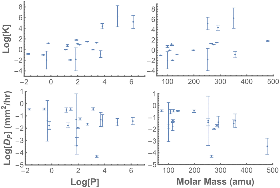 | ||
| Fig. 7 Correlations of PDMS-interaction parameters with select chemical properties. (Top) The PDMS–water partition coefficient (logK) generally increases with increasing logP, i.e. increasing hydrophobicity, and with increasing molar mass. No relationship is observed with H-bond donor count. (Bottom) Diffusivity in PDMS (logDP) generally decreases with increasing molar mass. No relationship is observed with logP or H-bond donor count. | ||
Extremely hydrophobic chemicals in microfluidic channels
Although indole served as a good test of our modeling approach, specifically because it partitions modestly into PDMS and thus has interesting flow- and time-dependent behaviors, many organ-on-chip users have greater concerns about the bioavailability of extremely hydrophobic compounds. We thus simulated constant flow at 10 μL min−1 through the same microfluidic channel as above for two additional sets of chemicals: a group of seven polychlorinated biphenyls (PCBs), with previously reported values for logKPW and logDP;44,45,54 and a group of seven polybrominated diphenyl ethers (PBDEs), with previously reported values for logDP (ref. 55) and with xlogKPW values estimated using a QSPR model developed by Zhu et al.45 All of these chemicals diffuse through PDMS at a similar rate as indole (logDP = −0.61 to −1.24 compared to −1.25) but partition into PDMS several orders of magnitude more strongly: logKPW = 4.43 to 8.67 compared to 0.91 (compiled in Table S3†).
Simulations based on these parameters show that PCBs and PBDEs would partition strongly out of a microfluidic channel and would diffuse quickly and deeply into the surrounding PDMS. As long as the inlet concentration was sufficiently dilute to realize full partitioning at the device's water–PDMS surfaces, then the bulk PDMS would continue sequestering more and more of these compounds for over a full week of simulated flow (Fig. S5A†). Even at such long times, over 98.7% of each PCB or PBDE is predicted to be lost from solution as it flows through the channel (Fig. S5B and C†). Such extremely hydrophobic compounds are not likely to be compatible with PDMS-based devices without additional modifications either to the polymer or the solution.
Discussion
We first investigated the PDMS interactions of ten chemicals, all reasonably hydrophobic (logP ≥ 1.9), but otherwise varying in structure and properties. Seven of these that interact with PDMS, and we fully characterized their interactions in a manner appropriate for 3D finite-element modeling. We then performed additional experiments with one chemical (indole) to confirm that such modeling accurately predicts time- and flow-rate-dependent doses in a PDMS-based microchannel. The agreement between model and experiment is good and confirms the validity of the overall approach.
Within this initial set of chemicals, the two key interaction parameters – the PDMS–water partition coefficient, KPW, and the diffusion constant in PDMS, DP – each vary over several orders of magnitude. A mapping of these results into DP–K parameter space is shown in Fig. 4. Notably, we find that six of these seven chemicals have DP values within the same order of magnitude (0.01–0.1 mm2 h−1). Interestingly, this range matches that for self-diffusion of PDMS chains.56 In this initial test set, rhodamine B stands alone as a slow diffusing outlier (4 × 10⁻⁴ mm2 h−1), and we confirmed its slow diffusion by direct imaging.
In our methods, we chose to measure concentration in solution using UV-vis spectroscopy, a convenient and accessible method for most laboratories. One drawback of this approach is that poorly water soluble chemicals with low molar absorptivity may have maximum concentrations below the limit of detection. For these cases, we developed and validated an approach in which measurements are taken for mixtures with high cosolvent fractions and then extrapolated to 0 and 100% cosolvent using a log-linear relationship. One can use the same log-linear relationship to estimate the relevant PDMS-interaction parameters in solutions in regimes more compatible with the biological requirements of cells, e.g., 0.1–5% DMSO by volume. We applied these methods for two chemicals, benzo[a]pyrene and chlorpyrifos, that are extremely hydrophobic and poorly soluble in water (solubilities of 1.62 μg L−1 and 1.4 mg L−1, respectively, at 25 °C). We found that the extrapolated partition coefficients agree with those previously reported using more sensitive but less accessible detection methods: logKPW = 5.20 ± 1.22 versus 5.27 ± 0.44 for benzo[a]pyrene; and logKPW = 6.25 ± 1.98 versus 4.31 ± 0.50 for chlorpyrifos.45 This agreement gives us confidence in the validity and usefulness of the log-linear extrapolation.
This method of extrapolation was also used for a third chemical, parathion, but for a different reason. Parathion is sufficiently soluble in water (20 mg L−1 at 25 °C) that its concentration could be measured using UV-vis spectroscopy; however, in experiments with little or no cosolvent (up to 20% DMSO by volume), parathion partitioned so strongly into PDMS that it reached a saturating concentration of approximately 3.2 mM or one parathion molecule per 520 nm3 of PDMS (Fig. S3†). We avoided this saturation regime by using higher DMSO fractions and extrapolating back to estimate a partition coefficient in pure aqueous solution: logKPW = 4.39 ± 0.50. This estimate is significantly higher than those from prior studies on parathion: logKPW ∼ 3;57,58 however, careful review of the methods from previous studies suggests that they were operating in the saturation regime and thus measured a lower effective partition coefficient. Based on the results here, a saturating concentration of parathion in PDMS can be reached when an adjacent pure aqueous solution has a concentration as low as 0.13 μM. Thus, the log-linear extrapolation is also useful for identifying the limits where linear water–PDMS partitioning breaks down.
All of the chemical–PDMS interaction parameters above were measured in specific geometries under no-flow conditions. To evaluate whether these parameters remain valid descriptors for different geometries and non-zero flow rates, we performed additional experiments in which a chemical solution flowed continuously through a PDMS microchannel. Indole was chosen for this test based on its combination of good water solubility, moderate partitioning, and quick diffusion through PDMS. When the relative indole concentration was measured at the microchannel outlet (Coutlet/Cinlet), it agreed well with the predictions of finite-element models that applied the previously determined PDMS-interaction parameters to this new geometry under two different flow rates. The PDMS-interaction parameters from static experiments can thus be used in a finite-element-based, toxicokinetic model to predict in-device concentrations under continuous perfusion.
Such FEM approaches have practical utility. They can be used to model in-device concentration profiles that cannot be measured directly due to the limited (few-μL) volume of a microchannel, e.g., the expected gradient of increased absorption/adsorption at the channel inlet compared to its outlet. These models can also be used to predict in-device bioavailability of compounds, such as we have done for PCBs and PBDEs. In this latter case, modeling showed that the extreme hydrophobic partitioning and rapid diffusion of these compounds in PDMS allows their continuing sequestration even for week-long exposures. It is just not possible to saturate the PDMS bulk, and thus keep more of the compounds in solution, on reasonable time scales for experiments.
With this approach validated for flow-through experiments, we measured PDMS-interaction parameters for an additional set of fourteen chemicals. Three of these showed no interaction with or penetration into PDMS – colchicine, bromophenol blue, and imazaquin. The remaining eleven all diffused through a PDMS membrane. Interestingly, seven of these eleven had logKPW ≤ 0, implying unfavorable partitioning into PDMS, and yet had large DP values from 0.04–0.36 mm2 h−1. This set represents a new and interesting class of chemicals: those that partition weakly into PDMS but diffuse through it quickly. Such chemicals pose a particular complication for microfluidic devices, namely cross-talk between parallel channels. Further, since several members of this chemical class had modestly positive or even negative logP, it suggests that the previously stated thresholds of logP ≤ 1.2 (ref. 24) or 1.8.22 do not necessarily limit chemical–PDMS interactions.
Using the combined set of 20 interacting chemicals, we can also look for correlations between chemical–PDMS interaction parameters and chemical properties (Fig. 7). Overall, logKPW is positively correlated with both logP and molar mass; and logDP is negatively correlated with molar mass. Despite earlier work suggesting a link between chemical loss into PDMS and hydrogen bond donor count,22 the data presented here do not have any such correlation. These results are not surprising: they merely suggest that more hydrophobic chemicals partition more favorably into PDMS, and that smaller molecules diffuse more quickly through PDMS. Nonetheless, our results do suggest that the interaction parameters behave as expected, and that a sufficiently large dataset could be used to build quantitative structure–property relationship (QSPR) models.
On the other hand, one has to be careful in using simple read-across methods to predict chemical–PDMS interactions based on analogs: chemicals with similar molecular properties can display markedly different interactions with PDMS. In our test set, we have three chemical pairs that are reasonably similar to one other: fluorescein and FITC; rhodamine B and rhodamine 6G; and parathion and paraoxon. A fourth pair, FITC and amodiaquine, are not structurally similar, but FITC has been used previously as an analog to estimate amodiaquine's PDMS-interaction parameters.33 In the case of fluorescein and FITC, the molecules share a similar structure, and neither show any interaction with PDMS. In the case of rhodamine B and rhodamine 6G, the molecules are members of the same dye family with almost identical masses and structures; however, rhodamine B partitions into and diffuses through PDMS, while rhodamine 6G only binds to the PDMS surface. In the case of paraoxon and parathion, the molecules only differ by a single atom replacement of sulfur for oxygen. Despite this similarity, paraoxon partitions into PDMS much more weakly than parathion; the two compounds have partition coefficients that differ by two orders of magnitude. Finally, in the case of amodiaquine and FITC, the two compounds have very different structures, but share similar molecular weights and logP values. Based of these similarities, the fluorescent dye FITC has been previously used as an analog for estimating the PDMS interactions of amodiaquine.33 Here, we measured the interactions directly for both compounds: FITC shows no interaction with PDMS in either disk soak, membrane, or optical diffusion experiments, but amodiaquine does partition into and diffuse within PDMS. Read-across methods may become better as we learn more about the molecular structure properties that determine chemical–PDMS interaction parameters, but analogs based solely on logP and molar mass are insufficient.
Ultimately, we have developed easily adoptable methods to determine chemical–PDMS interaction parameters from simple, static experiments. These parameters can then be used in finite-element models to calculate chemical concentration profiles for any user-defined channel geometry and flow rate. In fact, for simple geometries, the full finite-element models are well-approximated by heuristic models. Further, since our measured PDMS-interaction parameters are in good agreement with those previously reported (when such reports exist), one could reasonably take previously reported values of KPW and DP for other chemicals and apply them to 3D finite-element models to estimate in-device concentrations for any particular microfluidic device. Finally, recognizing that there is a strong push to replace PDMS with other materials, the same methods and model structure could be applied to alternative-material devices if the interaction parameters were measured for the new material.
Conclusions
We have developed methods to characterize the chemical–PDMS interaction parameters needed to model the distribution of a chemical of interest when an aqueous solutions is in contact with PDMS. We have measured these physical parameters for 24 hydrophobic chemicals, and confirmed the validity of these measurements through both direct observation of diffusion in PDMS and accurate predictions of time-dependent chemical loss in a PDMS-based microfluidic device. We find that partition coefficients and diffusion constants in PDMS can vary by orders of magnitude, and although there are trends with logP, with the number of hydrogen-bond donors, and with molar mass, one must exercise caution when using chemical analogs to infer PDMS-interaction parameters. With the battery of experiments and models presented here, one can measure chemical–PDMS interactions, even for highly hydrophobic compounds, and predictively model the time-dependent spatial distribution of a chemical of interest throughout the channels and PDMS bulk of a microfluidic device.
Abbreviations
| DMSO | Dimethyl sulfoxide |
| FEM | Finite element model(ing) |
| FITC | Fluorescein-5-isothiocyanate |
| IVIVE | In vivo–in vitro extrapolation |
| OoC | Organ-on-chip |
| PBDE | Polybrominated diphenly ether |
| PBS | Phosphate buffered saline |
| PCB | Polychlorinated biphenyl |
| PDMS | Polydimethylsiloxane |
| QSPR | Quantitative structure–property relation |
Definitions
| c S | Concentration in solution |
| c S1 | Concentration in source |
| c S2 | Concentration in sink |
| c P | Concentration in PDMS |
| D S | Diffusivity in solution |
| D P | Diffusivity in PDMS |
| H | Mass-transfer coefficient |
| K | Partition coefficient |
| K PW | PDMS–water partition coefficient |
| K PC | PDMS–cosolvent partition coefficient |
| K PM | PDMS–mixed solution partition coefficient |
| K PD | PDMS–DMSO partition coefficient |
| f | Volume fraction in solution |
| σ | Gaussian square width |
Data availability
Data for this article, including the results of disk and membrane soak experiments, and simulated solutions used in generating interpolation functions, are available at Open Science Framework at https://osf.io/892mf/.Conflicts of interest
There are no conflicts of interest to declare.Acknowledgements
This publication was supported by U.S. EPA STAR Center Grant #84003101. Its contents are solely the responsibility of the grantee and do not necessarily represent the official views of the U.S. EPA. Further, U.S. EPA does not endorse the purchase of any commercial products or services mentioned in the publication. The authors would also like to thank Phillip Fryman for his technical assistance.Notes and references
- B. H. Jo, L. M. V. Lerberghe, K. M. Motsegood and D. J. Beebe, J. Microelectromech. Syst., 2000, 9, 76–81 CAS.
- S. K. Sia and G. M. Whitesides, Electrophoresis, 2003, 24, 3563–3576 CrossRef CAS PubMed.
- S. Halldorsson, E. Lucumi, R. Gómez-Sjöberg and R. M. Fleming, Biosens. Bioelectron., 2015, 63, 218–231 CrossRef CAS PubMed.
- M. S. Hutson, P. G. Alexander, V. Allwardt, D. M. Aronoff, K. L. Bruner-Tran, D. E. Cliffel, J. M. Davidson, A. Gough, D. A. Markov, L. J. McCawley, J. R. McKenzie, J. A. McLean, K. G. Osteen, V. Pensabene, P. C. Samson, N. K. Senutovitch, S. D. Sherrod, M. S. Shotwell, D. L. Taylor, L. M. Tetz, R. S. Tuan, L. A. Vernetti and J. P. Wikswo, Appl. In Vitro Toxicol., 2016, 2(2), 97–102 CrossRef.
- K. S. Nitsche, I. Müller, S. Malcomber, P. L. Carmichael and H. Bouwmeester, Arch. Toxicol., 2022, 96, 711–741 CrossRef CAS PubMed.
- I. Miranda, A. Souza, P. Sousa, J. Ribeiro, E. M. Castanheira, R. Lima and G. Minas, J. Funct. Biomater., 2022, 13, 2 CrossRef CAS PubMed.
- Y. Yang, Y. Chen, L. Wang, S. Xu, G. Fang, X. Guo, Z. Chen and Z. Gu, Front. Bioeng. Biotechnol., 2022, 10, 900481 CrossRef PubMed.
- D. Singh, A. Mathur, S. Arora, S. Roy and N. Mahindroo, Appl. Surf. Sci. Adv., 2022, 9, 100246 Search PubMed.
- Emulate, Organ-Chip Consumables, 2024, https://emulatebio.com/organ-chip-consumables/ Search PubMed.
- S. P. Deosarkar, B. Prabhakarpandian, B. Wang, J. B. Sheffield, B. Krynska and M. F. Kiani, PLoS One, 2015, 10(11), e0142725 CrossRef PubMed.
- S. Pradhan, A. M. Smith, C. J. Garson, I. Hassani, W. J. Seeto, K. Pant, R. D. Arnold, B. Prabhakarpandian and E. A. Lipke, Sci. Rep., 2018, 8, 3171 CrossRef PubMed.
- T. D. Brown, M. Nowak, A. V. Bayles, B. Prabhakarpandian, P. Karande, J. Lahann, M. E. Helgeson and S. Mitragotri, Bioeng. Transl. Med., 2019, 4, e10126 Search PubMed.
- Z. Liu, S. Mackay, D. M. Gordon, J. D. Anderson, D. W. Haithcock, C. J. Garson, G. J. Tearney, G. M. Solomon, K. Pant, B. Prabhakarpandian, S. M. Rowe and J. S. Guimbellot, Biomed. Opt. Express, 2019, 10, 5414–5430 CrossRef CAS PubMed.
- S. Köhler, C. Benz, H. Becker, E. Beckert, V. Beushausen and D. Belder, RSC Adv., 2012, 2, 520–525 RSC.
- A. L. Nair, L. Mesch, I. Schulz, H. Becker, J. Raible, H. Kiessling, S. Werner, U. Rothbauer, C. Schmees, M. Busche, S. Trennheuser, G. Fricker and M. Stelzle, Biosensors, 2021, 11, 314 Search PubMed.
- Micronit, Organ-on-a-Chip platforms, 2024, https://micronit.com/product-spotlight/organ-on-a-chip Search PubMed.
- J. C. McDonald, D. C. Duffy, J. R. Anderson, D. T. Chiu, H. Wu, O. J. Schueller and G. M. Whitesides, Electrophoresis, 2000, 21, 27–40 Search PubMed.
- M. W. Toepke and D. J. Beebe, Lab Chip, 2006, 6, 1484–1486 RSC.
- J. D. Wang, N. J. Douville, S. Takayama and M. ElSayed, Ann. Biomed. Eng., 2012, 40, 1862–1873 CrossRef PubMed.
- B. J. van Meer, H. de Vries, K. S. Firth, J. van Weerd, L. G. Tertoolen, H. B. Karperien, P. Jonkheijm, C. Denning, A. P. IJzerman and C. L. Mummery, Biochem. Biophys. Res. Commun., 2017, 482, 323–328 CrossRef CAS PubMed.
- N. Convery and N. Gadegaard, Micro Nano Eng., 2019, 2, 76–91 Search PubMed.
- A. W. Auner, K. M. Tasneem, D. A. Markov, L. J. McCawley and M. S. Hutson, Lab Chip, 2019, 19, 864–874 RSC.
- P. N. Carlsen, Polydimethylsiloxane: Structure and Applications, NOVA Science, 2020 Search PubMed.
- A. M. Kemas, R. Z. Shafagh, N. Taebnia, M. Michel, L. Preiss, U. Hofmann and V. M. Lauschke, Adv. Healthcare Mater., 2024, 13, 2303561 Search PubMed.
- R. Prantil-Baun, R. Novak, D. Das, M. R. Somayaji, A. Przekwas and D. E. Ingber, Annu. Rev. Pharmacol. Toxicol., 2018, 58, 37–64 Search PubMed.
- D. R. Miller, E. S. McClain, J. N. Dodds, A. Balinski, J. C. May, J. A. McLean and D. E. Cliffel, Front. Bioeng. Biotechnol., 2021, 9, 622175 Search PubMed.
- S. E. Eklund, D. E. Cliffel, E. Kozlov, A. Prokop, J. Wikswo and F. Baudenbacher, Anal. Chim. Acta, 2003, 496, 93–101 Search PubMed.
- J. R. McKenzie, D. E. Cliffel and J. P. Wikswo, in Electrochemical Monitoring of Cellular Metabolism, Springer, 2014, pp. 522–528 Search PubMed.
- K. L. Bruner-Tran, J. Gnecco, T. Ding, D. R. Glore, V. Pensabene and K. G. Osteen, Reprod. Toxicol., 2017, 68, 59–71 Search PubMed.
- V. R. Stephens, J. T. Rumph, S. Ameli, K. L. Bruner-Tran and K. G. Osteen, Front. Physiol., 2022, 12, 807685 Search PubMed.
- L. Richardson, J. Gnecco, T. Ding, K. Osteen, L. M. Rogers, D. M. Aronoff and R. Menon, Reprod. Sci., 2020, 27, 1933719119828084 Search PubMed.
- L. Si, H. Bai, M. Rodas, W. Cao, C. Y. Oh, A. Jiang, R. Moller, D. Hoagland, K. Oishi, S. Horiuchi, S. Uhl, D. Blanco-Melo, R. A. Albrecht, W. C. Liu, T. Jordan, B. E. Nilsson-Payant, I. Golynker, J. Frere, J. Logue, R. Haupt, M. McGrath, S. Weston, T. Zhang, R. Plebani, M. Soong, A. Nurani, S. M. Kim, D. Y. Zhu, K. H. Benam, G. Goyal, S. E. Gilpin, R. Prantil-Baun, S. P. Gygi, R. K. Powers, K. E. Carlson, M. Frieman, B. R. tenOever and D. E. Ingber, Nat. Biomed. Eng., 2021, 5, 815–829 CrossRef CAS PubMed.
- J. Grant, A. Özkan, C. Oh, G. Mahajan, R. Prantil-Baun and D. E. Ingber, Lab Chip, 2021, 21, 3509–3519 Search PubMed.
- D. A. Markov, J. Q. Lu, P. C. Samson, J. P. Wikswo and L. J. McCawley, Lab Chip, 2012, 12, 4560–4568 Search PubMed.
- S. Schneider, E. J. Brás, O. Schneider, K. Schlünder and P. Loskill, Micromachines, 2021, 12, 575 Search PubMed.
- S. Kim, J. Chen, T. Cheng, A. Gindulyte, J. He, S. He, Q. Li, B. A. Shoemaker, P. A. Thiessen, B. Yu, L. Zaslavsky, J. Zhang and E. E. Bolton, Nucleic Acids Res., 2023, 51, D1373–D1380 Search PubMed.
- S. B. Campbell, Q. Wu, J. Yazbeck, C. Liu, S. Okhovatian and M. Radisic, ACS Biomater. Sci. Eng., 2021, 7, 2880–2899 CrossRef CAS PubMed.
- U. M. Cao, Y. Zhang, J. Chen, D. Sayson, S. Pillai and S. D. Tran, Int. J. Mol. Sci., 2023, 24, 3232 CrossRef CAS PubMed.
- B. Kim, E. T. Peterson and I. Papautsky, The 26th Annual International Conference of the IEEE Engineering in Medicine and Biology Society, 2004, pp. 5013–5016 Search PubMed.
- J. Zhou, A. V. Ellis and N. H. Voelcker, Electrophoresis, 2010, 31, 2–16 Search PubMed.
- D. A. Markov, E. M. Lillie, S. P. Garbett and L. J. McCawley, Biomed. Microdevices, 2014, 16, 91–96 Search PubMed.
- B. D. Chapron, A. Chapron, B. Phillips, M. C. Okoli, D. D. Shen, E. J. Kelly, J. Himmelfarb and K. E. Thummel, Altex, 2018, 35, 504–515 Search PubMed.
- F. C. Fischer, L. Henneberger, R. Schlichting and B. I. Escher, Chem. Res. Toxicol., 2019, 32, 1459–1468 Search PubMed.
- A. Belles, C. Franke, C. Alary, Y. Aminot and J. W. Readman, Environ. Toxicol. Chem., 2018, 37, 1291–1300 CrossRef CAS PubMed.
- T. Zhu, W. Chen, H. Cheng, Y. Wang and R. P. Singh, Ecotoxicol. Environ. Saf., 2019, 182, 109374 Search PubMed.
- F. Schneider, T. Fellner, J. Wilde and U. Wallrabe, J. Micromech. Microeng., 2008, 18, 065008 Search PubMed.
- J. N. Lee, C. Park and G. M. Whitesides, Anal. Chem., 2003, 75, 6544–6554 CrossRef CAS PubMed.
- J. Crank, The Mathematics of Diffusion, Oxford University Press, 2nd edn, 1975 Search PubMed.
- J. C. Jaegar and H. S. Carslaw, Conduction of Heat in Solids, Oxford University Press, 2nd edn, 1986 Search PubMed.
- J. Seader, E. J. Henley and D. K. Roper, Separation Process Principles: Chemical and Biochemical Operations, Wiley, 3rd edn, 2011 Search PubMed.
- S. H. Yalkowsky and J. T. Rubino, J. Pharm. Sci., 1985, 74, 416–421 CrossRef CAS PubMed.
- S. Miyamoto and K. Shimono, Molecules, 2020, 25, 5340 CrossRef CAS PubMed.
- EPA, TSCA Work Plan for Chemical Assessments: 2014 Update, 2014 Search PubMed.
- T. P. Rusina, F. Smedes and J. Klanova, J. Appl. Polym. Sci., 2010, 116(3), 1803–1810 CrossRef CAS.
- J. F. N. Valderrama, K. Baek, F. J. Molina and I. J. Allan, Environ. Sci.: Processes Impacts, 2016, 18, 87–94 RSC.
- L. Garrido, J. E. Mark, J. L. Ackerman and R. A. Kinsey, J. Polym. Sci., Part B: Polym. Phys., 1988, 26, 2367–2377 CrossRef CAS.
- S. Magdic, A. Boyd-Boland, K. Jinno and J. B. Pawliszyn, J. Chromatogr. A, 1996, 736, 219–228 Search PubMed.
- D. A. Lambropoulou, V. A. Sakkas and T. Albanis, Anal. Bioanal. Chem., 2002, 374, 932–941 CrossRef CAS PubMed.
Footnotes |
| † Electronic supplementary information (ESI) available. See DOI: https://doi.org/10.1039/d4lc00840e |
| ‡ Similar models for mass and heat transport have been well described and often have analytic or semi-analytic solutions for limited cases (e.g., for no flow and infinite or semi-infinite domains). We proceed with numerical solutions, but approximate analytic solutions can be derived under well-mixed solution conditions (large DS) and certain simple geometries.48–50 |
| This journal is © The Royal Society of Chemistry 2025 |