In silico modeling enables greener analytical and preparative chromatographic methods

Abstract

Green analytical chemistry has garnered significant interest given the heightened focus for organizations to decrease their environmental footprint. Of the analytical methodologies, those involving separation science (chromatography, extractions, crystallization, etc.) tend to be the most detrimental to the environment as they require large volumes of solvent. Chromatographic methods can be made significantly greener while preserving their performance by changing the mobile phase and method conditions. However, this process is laborious and involves significant analyst time for experimentation and method refinement. Herein, we introduce in silico modeling and computer-assisted method development as a rapid, accurate, robust, and green technique to develop greener methods. For the first time, it is shown that the analytical method greenness score (AMGS) can be mapped across the entire separation landscape. This allows for methods to be developed based off their performance and greenness simultaneously. Given the increased scrutiny of fluorinated solvents, the utility of in silico modeling is demonstrated to move from a fluorinated mobile phase additive to an alternative chlorinated additive. Here, the AMGS is reduced from 9.46 to 4.49 while critical pairs go from fully overlapped to having a resolution of 1.40. Acetonitrile is also shown to be replaced in the mobile phase with environmentally friendlier methanol to reduce the AMGS from 7.79 to 5.09 while preserving the critical resolution. Finally, we demonstrate the use of a resolution map to capitalize on peak crossover and increase the loading of an active pharmaceutical ingredient by 2.5× in a preparative chromatography setting. This results in 2.5× less replicates needed during the purification. This study provides a framework that separation scientists can apply to green chromatographic separations using in silico modeling.

---

1. Introduction

Techniques involving separation science (dominated by liquid chromatography [LC]) are particularly detrimental to the environment as they use large amounts of pure solvent, and electrical power to work against entropy and isolate constituents from complex mixtures.^1–3 Analytical chromatography, although perceived as less detrimental compared to preparative chromatography, is a prolific pollution generator.^2–4 For example, some major pharmaceutical companies have been reported to operate more than one thousand high performance liquid chromatography (HPLC) systems alone, each traditionally producing ∼1 L of waste per day.² Analytical separations are ideally conducted in capillaries, which require far less solvent, through capillary electrophoresis, or capillary liquid chromatography.^3,5,6 However, the practical limitations of these techniques such as poor reproducibility, proneness to clog, and limited sample capacity limit their use today making research into greening traditional analytical HPLC needed. Preparative chromatography (flash/high performance) is indispensable for drug discovery and organic synthesis (μg to kg scale) workflows, and can generate >5 L min⁻¹ of solvent from a preparative HPLC.⁷ Traditionally, chromatographic methods are developed through experimental trials with iterative refinement. The innumerable physicochemical interactions that occur during a separation make method development experimentally demanding and can hinder sustainable development.

To develop a green method, there must be an understanding of how to quantify a method's greenness just like any other analytical figure of merit (resolution, retention, selectivity etc.).^8–11 Greenness is a relative construct where methods, solvents, or both are more or less green depending on the parameters considered.¹² To this extent, there has been an array of green analytical chemistry (GAC) metrics and constructs recently published to assist researchers in quantifying and understanding their method's greenness.^9,13–15 A useful metric for chromatography is the analytical method greenness score (AMGS) which was introduced in 2019 as part of the American Chemical Society's Green Chemistry Institute Pharmaceutical Roundtable (ACS-GCI-PR).¹⁶ Analysis of the AMGS shows that greening chromatography (without changing hardware) can be performed by making separations faster (reducing instrument energy consumption and/or peak volumes), applying greener solvents/additives, or both.^3,4 An important tool, that is not often discussed for its greenness, is in silico chromatographic modeling which can be used to accelerate green method development and achieve these goals rapidly.

With data from limited experimentation, in silico modeling maps the separation landscape and allows for optimization of method conditions with excellent predicative capabilities.¹⁷ Today's models are capable of considering multiple factors including the effects of: gradient time/shape, instrument dwell volume, mobile phase composition, mobile phase pH, and column temperature.¹⁸ The modeling is effective for gas chromatography, reversed phase LC (RPLC), normal phase LC (NPLC), sub/supercritical fluid chromatography (SFC), and more for complex samples of small and large molecules.^19–23 This technology is inherently green as it reduces experimentation during method development, however it is rarely systematically studied in the context of green analytical chemistry. Herein, we demonstrate the use of in silico modeling for facile greening of analytical and preparative liquid phase separations. Mapping of the separation space in terms of not only resolution but also greenness is achieved for the first time. Recent regulatory rulings in Europe have proposed banning the use of per- and polyfluoroalkyl substances (PFAS) which are termed as ‘forever chemicals’ due to their detrimental impact on health and extreme environmental persistence. Trifluoroacetic acid, one of the most used additives in liquid chromatography falls into the category of PFAS. Using in silico method development, a switch from trifluoroacetic acid to trichloroacetic acid is made possible while positively impacting chromatographic figures of merit. The rapid substitution of a less green solvent (acetonitrile) with a greener solvent (methanol) using this technology is demonstrated. Finally, in silico modeling is used to isolate a dimerized active pharmaceutical ingredient (API) from Amgen's pipeline to increase loading and green a preparative separation. We aim to demonstrate not only improvement of the AMGS, but also analytical performance simultaneously via in silico modeling instead of experimentation.

2. Experimental

2.1 Materials

Acetaminophen (>98%), Acetazolamide (98%), carbamazepine (98%), sulfathiazole (98%), and theobromine (98%) were from AA Blocks (San Diego, CA, USA). Tolnaftate (99%) was from AK Scientific (Union City, CA, USA). Solvents were from Fisher Scientific (Waltham, MA, USA) as LC-MS grade with 0.1% (v/v) additive already added to the solvent, when desired. The trichloroacetic acid (TCA) mobile phase was prepared manually, and the (TCA) was from Oakwood Products (>99%, Estill, SC, USA).

2.2 Chromatography

All separations were conducted on an Agilent Technologies (Santa Clara, CA, USA) 1290 UHPLC-MS. The instrument had two valve driver units (G1170A) used to select the mobile phase of interest, a high-speed pump (G7120A), two multicolumn thermostats (G7116B) with 7 column positions per compartment and a bypass position in both, a diode array detector (G7117A), and a single quadrupole mass spectrometer (G6125B). The instrument was controlled by Agilent's OpenLab for ChemStation (Rev. 2.01.10[287]). The Pack Pro C18 column was used for all examples shown and was purchased from YMC (Devens, MA, USA) in the dimensions of 100 mm × 3.0 mm (i.d.) with 3.0 μm particles. Chromatographic resolutions in the manuscript were calculated via the width at half height method in PeakLab (v.1.05.02, AIST Software Inc., Mapleton, OR, USA) using the Gen2HVL function on baseline corrected chromatograms.

2.3 Modeling methodologies

In silico modeling was performed using LC Simulator 2019 (version L05R41) from ACD Labs (Advanced Chemistry Development, Toronto, Ontario, Canada). AMGS calculations were done in the MATLAB (R2023a, The MathWorks Inc., Natick, MA, USA) environment using eqn (1). The following version of the AMGS that focuses solely on chromatography,where R is the number of replicate analysis required by the method, t_a is the time of analysis, t_c is the cycle time (time in between analysis ending and the next starting²⁴), F is the flow rate, S is the safety health and environment index of the mobile phase solvent(s), C is the cumulative energy demand of the mobile phase solvent(s), E is the energy demand of the chromatograph, and N is the number of analytes in the sample.⁴ The S, C, and E (density corrected for solvents) values for a variety of solvents and instruments have been published elsewhere^3,4 and an automated version of the AMGS calculator is provided by the ACS online (https://www.acsgcipr.org/amgs/). For gradient elution, or multicomponent isocratic mobile phases, the C and S constants should be an average value weighted by volume. A two minute re-equilibrium was allowed for each method in this paper, where 60 s of the re-equilibrium occurred during the instrument's cycle time (t_c). The AMGS is considered unitless for practical use, and lower values indicate a greener method.

To construct the AMGS map (Fig. 1B), LC Simulator was used to calculate the run times of 80 different methods (8 temperatures, 10 gradient times) across the separation space. Using the run times, gradient time, and gradient composition the code calculated the volume of solvent A and B used each of the 80 methods. The AMGS was then calculated using volume weighted values for C and S (eqn (1)) for all 80 data points. The 2-D AMGS scattered data was formed into a matrix and interpolated to 100 × 100 using the ‘griddata’ function with triangulation-based cubic (‘cubic’) interpolation. The interpolated data was then plotted as a filled contour plot (‘countourf’) with 1000 data levels. An example dataset (Fig. 1) and full code are provided as ESI† for reproducibility.

Fig. 1 (A) An example resolution map where gradient time (min) is plotted on the x-axis, column temperature (°C) is plotted on the y-axis and critical resolution is plotted on the z-axis (colorbar) for a degradation solution with 11 analytes analyzed by RPLC. Critical resolution is defined as the resolution between the two closest peaks in the chromatogram. (B) A map of each method's sustainability across the separation space represented by the AMGS (z-axis) for the same separation as A with the same x- and y-axes. Lower AMGS values indicate a greener method. (C) Calculated numerical description for four different methods in different spaces of the separation landscape. Conditions: 100 mm × 3.0 mm PackPro C18 with 3 μm particles, 0.4 mL min⁻¹, 38–68% B in 1.2, 7, 12, 18 minutes with hold times of 4.8, 23.5, 22.4, and 21.2 minutes respectively. A = 0.1% TFA in H₂O, B = MeOH, 254 nm UV detection.

3. Results and discussion

3.1 Mapping the resolution and sustainability of a separation landscape

Software have been commercialized (DryLab, LC Simulator, etc.) that can accurately model how analytes migrate during the separation process and predict the resulting chromatogram in response to experimental factors such as temperature, gradient shape/time and ionic strength. In general, these software use a training set of retention times (t_r) (along with peak widths, and peak asymmetries to predict resolutions) to calculate retention factors on a column with a given dead time (t₀). After calculation of retention factors, proprietary equations are applied to relate log(k) to organic composition (%B), column temperature (t), and ionic strength of the mobile phase.⁵² To generate a model's training data set, a 3 × 3 screening protocol is firstly employed, where three linear gradients are used ranging from 5% B to 95% B in 4, 8, and 12 minutes at 25, 35 and 60 °C. Using this data, the software can map out the separation landscape and predict peak locations, widths, and shapes at different experimental conditions. The software can simulate the chromatogram under any condition within the space at the click of a button. The first output of the software is a “resolution map” of the “screening space” showing how critical resolution (R_{S Critical}) changes when the same 5% to 95% B linear gradient is used with different gradient times and temperatures. For these maps, gradient time (min) is plotted on the x-axis, column temperature (°C) on the y-axis, and critical resolution on the z-axis. After the generation of the resolution map for the screening space, the in silico modeling can be used for optimization (automatically or guided by a user) to generate experimental conditions with different %B starting and ending points, gradient times, different temperatures, and multi-step gradients, if needed, to produce the required result.

A representative resolution map for the screening space is shown in Fig. 1A for a degradation solution with eleven components. The gradients for this map start at 38% B and end at 68% B. This sample was analyzed using a C18 column (YMC Pack Pro C18). When analyzing a resolution map, areas with orange/red result in the highest resolution for the critical pair. Mixtures whose constituents are structurally diverse, such as those in this sample, are known as “irregular” samples.²⁵ In irregular samples, analytes can react to experimental changes (within the same system) with different magnitudes, causing elution order changes known as “peak crossover”.²⁰ Peak crossover cannot occur for “regular” samples whose analytes are structurally similar. Method development in the presence of peak crossover is challenging and laborious, however by using in silico modeling crossover is immediately visualized on the resolution map through dark blue strips (R_{s Critical} = 0) surrounded by yellow or orange (larger R_{s Critical}).²⁰ Multiple critical pairs crossover in Fig. 1A, making several locations within the screening space (experimental conditions) offer baseline resolution (R_{S Critical} > 1.5, orange). One substantial benefit of preparing a resolution map is the ability to quantify the solvent demand (of all gradient components) and run time for each discretized point across the separation space. As a result, sustainability can be “mapped” as easily as critical resolution.

To map the sustainability of a separation space, a metric must be chosen to quantify the greenness of each computed method across the space. The development and refinement of GAC metrics, constructs, and models has become a field of research in its own.^{13–15,26–31} Although, many tools from these efforts have their own merit, we will use the analytical method greenness score (AMGS) to discuss a method's greenness.^16,32 The AMGS is an open-access comprehensive tool that can be used to calculate the greenness of sample/standard preparation, chromatography, or both. In Fig. 1B, the AMGS is mapped (see section 2.3 for details) across the screening space for the same separation whose resolution was mapped in Fig. 1A. With this map, the AMGS at any temperature or gradient time can be provided by the clicking on that spot of the map. In Fig. 1B, the AMGS ranges from >25 to less than <5 showing a >5× change in greenness across the screening space even when using the same hardware, mobile phase components, and gradient start/end compositions. In general, AMGS maps will show a similar trend as Fig. 1B with greener methods (lower AMGS, blue) produced by faster elution (from hotter column temperature and shorter gradients) as this reduces solvent consumption and instrument power demands.⁴ It is important to note that the current version of the AMGS uses a constant value (E) for each instrument's power demand, and that if the E value was physically measured it would change from condition-to-condition and would favor separations conducted near ambient temperatures. This could potentially change the trend of the AMGS maps, and with time we expect the AMGS to continue to be refined becoming iteratively more accurate. When choosing the ideal method conditions, one should search for the location in their separation space that provides the minimum AMGS while providing adequate resolution.

To demonstrate how these maps can be used for GAC method development, four methods were chosen within this separation space (Fig. 1) listed as I–IV. After providing the temperature of the column and gradient time, the in silico model can calculate the run time and critical resolution that can be used to calculate the AMGS (Fig. 1C). All of the selected methods provide similar and suitable calculated critical resolutions (Fig. 1A, R_s = 1.47–1.87), yet their greenness differ drastically (Fig. 1B, AMGS = 3.34–17.4). Of these, method I would be the most “ideal” as it provides fast elution (analysis time 6.0), baseline resolution (1.65), and the lowest AMGS (3.34) of the evaluated methods. When choosing the ideal method, it is important to consider Nowak's RGB additive color model of GAC otherwise referred to as the “white analytical chemistry” (WAC) concept.^10,11 For the RGB/WAC model, a method's sustainability (green) is balanced with practicality (blue) and analytical performance (red) to make the ideal “white” method. On Fig. 1B, there are conditions that produce AMGSs as low as 2.83 (1 minute gradient, 80 °C), however, they provide very low resolution (R_S < 0.3) making them not high performing or practical. For a green method to be ideal, it must also serve its desired purpose.

3.2 Simultaneous replacement of a PFAS additive and improved analytical performance

Alternatively, in silico modeling can be used to develop new methods using different systems (mobile phase/stationary phase combinations) that are greener and/or meet new sustainability requirements. For example, a proposed EU law seeks to prohibit the manufacture, supply, and usage of a broad spectrum of per- and polyfluorinated alkyl substances (PFAS) materials, encompassing fluoroalkyl compounds irrespective of their molecular weight.³³ These “forever chemicals” include substances ranging from TFA to polymers like PTFE, PVDF, and Viton, with exceptions made for active pharmaceutical ingredients (API) molecules. The potential ramifications of such a ban on the chemical and (bio)pharma industries within Europe are considerable, and future legislation with a similar ban will likely be introduced in the United States. For instance, trifluoroacetic acid (TFA) remains the dominant mobile phase additive for reversed phase liquid chromatography (RPLC) of peptides and small molecules.³⁴ Its ubiquitous use underscores its critical role in analyses and purification processes. One limitation of the AMGS is that it excludes the impact of mobile phase additives, meaning a method's score will not rise due to the incorporation of TFA, even if TFA is harmful to the environment. Instead, the AMGS may be lowered due to quicker elution often seen in RPLC using TFA compared to weaker acids like acetic or formic acid. The Olesik group recently did an in depth life cycle analysis (LCA) to evaluate the AMGS’ omission and found that for small molecule SFC separations using TEA, the additive itself contributed very little to the method's overall sustainability.³⁵ There are GAC metrics that can consider the effects of additives such the newly released ChlorTox Scale which uses safety data sheets to calculate the total chemical risk.³¹ Regardless of the metric TFA, like all PFAS, is much more environmentally persistent than non-fluorinated compounds^36–38 and any legislation banning PFAS that include TFA would disrupt RPLC methodologies necessitating significant adjustments in chromatographic separations.

The use of in silico modeling will greatly aid in transferring methods that are currently using TFA to a non-fluorinated additives if needed, or in developing methods without TFA to start. Fig. 2A shows an example separation of a degradation sample in the reversed phase, using an H₂O/TFA and MeOH gradient from 5% to 95% in 24 minutes on a C18 column. With this screen, despite the long gradient time, there was complete overlap for two critical pairs (3&4 and 9&10). It was desired to make a method without TFA to operate without PFAS while improving the resolution of the peaks so that all 11 peaks can be individually quantitated. One alternative to TFA that has been shown to provide similar beneficial characteristics is trichloroacetic acid (TCA).³⁹ To start with method development, the 3 × 3 screen as discussed above was ran on this sample with 0.1% TCA in the mobile phase A, instead of 0.1% TFA. This data was modeled to produce a resolution map of the screening space as shown in Fig. 2B. Here, the complexity of this sample is shown with multiple critical pairs that crossover represented by dark blue stripes through orange areas. Resolution maps are often scaled to the resolution range obtained within the space, so that orange represents the highest resolution possible but not necessarily baseline resolution. When using a 5% to 95% B linear gradient, and TCA as an additive, the greatest critical resolution that can be achieved for gradient times 0 to 15 minutes and temperatures of 20 °C to 65 °C is ∼0.95 representing a split peak on the critical pair(s). If the screening space does not provide a suitable method, the in silico model can then be used for additional method optimization.

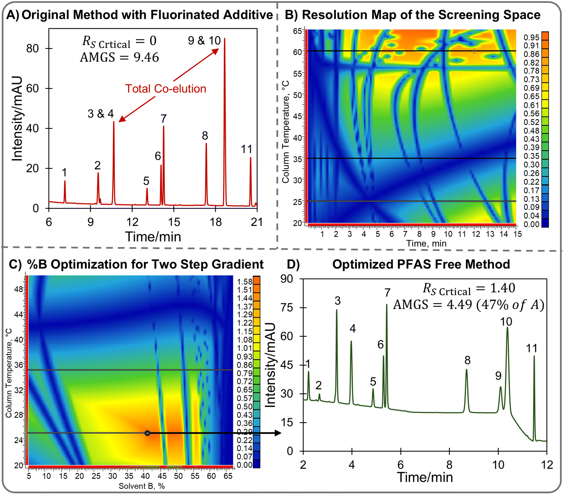Fig. 2 (A) Chromatogram showing the separation of a forced degraded pharmaceutical sample on a C18 column with a gradient 0–24 minutes 5% B to 95% B with A = 0.1% TFA in H₂O and B = MeOH. (B) Resolution map for the screening space (5% B to 95% B) of the same solution as (A) with 0.1% trichloroacetic acid (TCA) used as the additive instead of TFA in the water component of the mobile phase. (C) Resolution map optimizing the starting conditions of the mobile phase (% B on x-axis, °C on y-axis) for the separation with TCA in the water. (D) Optimized chromatogram with a multi-stepped gradient (0–5 minutes 41% B, 9 minutes–12 minutes 100% B) showing full resolution of all eleven components of interest and an AMGS 2.1× lower while removing the PFAS additive. Conditions: 100 mm × 3.0 mm PackPro C18 with 3 μm particles, 0.4 mL min⁻¹, 254 nm UV detection.

The LC simulator will automatically generate methods to achieve what is specified as “suitable” and provide a suitability score of 0 (does not meet requirements) to 1 (meets all requests). When setting method suitability options, the desired run time, resolution, gradient steepness, and other parameters can be defined. For difficult separations, such as the one in Fig. 2, gradients with multiple steps may be required along with isocratic holds at the start, end, or at multiple points during the method. When optimizing a method in silico, resolution maps can be generated for any point of time during the analysis. For example, Fig. 2C shows a resolution map that was used to optimize the separation in Fig. 2B. This resolution map is for time 0, optimizing the starting mobile phase composition. For this map, the x-axis represents the organic composition in the starting mobile phase (%B), not the gradient time as was plotted for the previously discussed maps. Notice that, if the gradient being examined started at 5% B, like the screening methods, very little resolution would be achieved (<0.2 for most column temperatures). However, starting at 41% B at 25 °C, presents the possibility for baseline resolution (Fig. 2C, orange). It is best to choose an area of the map in the center of orange regions, as these areas provide the most robust separation. The computer model predicted optimal conditions for the gradient to be 41% B at the start until 5 minutes before ramping to 67% B at 9 minutes and finishing at 100% B at 10 minutes that is held until 12 minutes. The result of this multi-stepped gradient is shown in Fig. 2D, where all 11 peaks are now separated in less time compared the TFA method (run time of 14 minutes instead of 30 minutes). The critical pair 9 and 10 now has a resolution of 1.40 showing a significant improvement compared to Fig. 2A. The switch to TCA did introduce an artifact in the slopped baseline present in Fig. 2D that is not as prominent with the TFA (Fig. 2A) which would require removal with a blank subtraction or mathematical baseline correction method. The AMGS of the PFAS free method is 4.49 (Fig. 2D) compared to 9.46 of the TFA screen (Fig. 2A) meaning the greenness is increased by 2.1×, while improving the method's performance simultaneously.

3.3 Substituting greener solvents

As TFA is often the most used effective additive for RPLC, acetonitrile (ACN) is considered the “gold standard” organic mobile phase component in RPLC. ACN has a large eluotropic strength, full miscibility with water, low viscosity when mixed with water, and a low UV cutoff.^4,35,40 The production of HPLC or LC-MS grade ACN is energy extensive requiring multiple steps making its cumulative energy demand (C, eqn (1)) value in the AMGS high (4.622 mL⁻¹) compared to the commonly used alcohols (MeOH C = 1.465 mL⁻¹ and EtOH C = 1.452 mL⁻¹) for RPLC mobile phases.^3,41 Therefore, it is beneficial to remove ACN from RPLC mobile phases and substitute it with a more energetically favorable solvent.^4,42 Additionally, ACN's multistep production often starts with materials that are acquired from other chemical processes, which when paused can lead to shortages such as the unexpected ACN shortage in 2008 now referred to as “The Great Acetonitrile Shortage”.^43,44 This shortage drove prices to unprecedented heights, prompting discussions across scientific communities and leading to concerns about price gouging and the reliability of alternative sources. In response to the crisis, laboratories, especially those in regulated industries like pharmaceuticals, were compelled to seek alternative solvent systems. The United States Food and Drug Administration (FDA) received numerous inquiries regarding the shortage, particularly concerning the substitution of alternative solvents in validated methods. The FDA emphasized the importance of method validation and compliance with good manufacturing practices (GMPs) regardless of any changes made to address the shortage.⁴³ The crisis encouraged a movement towards developing strategies for alternative solvent usage, including greener solvent systems and miniaturized chromatographic methods. In addition to ACN's production issues, mobile phase waste disposal for our departments is done through incineration and studies have shown that ACN incineration can contribute to the production of acid rain.⁴⁵

Transitioning to alternative solvents for the purpose of greenness or in a response to a shortage poses challenges, particularly relating to analyte selectivity and method validation when using lower performing solvents (such as MeOH for ACN).^46,47 Peak broadening and selectivity changes can occur during solvent substitution which complicates method development and places a large burden on the analysts. These challenges often lower the motivation to improve the sustainability of already developed methods. The use of in silico modeling can be quickly used to track changes in selectivity and develop methods with more sustainable and economical solvents. In Fig. 3A, the separation of 6 pharmaceutically relevant analytes on a reverse phase C18 column using a H₂O TFA/ACN gradient. Here, the AMGS is 7.79 and the critical resolution (peaks 3 and 4) is 1.59. The ACN was then replaced with MeOH and the 3 × 3 standard screen was conducted. As was the case for the TFA removal, there was no location in the screening space that provided baseline resolution so in silico optimization was initiated. The computer optimized method (Fig. 3C) suggested that the gradient start at 15% B which is held for 3 minutes before ramping to 100% B at 5 minutes that is held until the 7 minutes. Fig. 3B shows the resolution map for time zero, where low temperatures are required for the separation (<35 °C) with two areas of possible baseline resolution. The blue stripe splitting the areas of resolution represents peak 1's crossover of peak 3 where areas to the left of 20% B represent peak 1 eluting after peak 3 and areas to the right of 20% B predict peak 2 eluting before peak 3. The MeOH optimized method (Fig. 3C) shows baseline resolution for all six analytes (R_{S Critical} = 1.59 Peaks 2 and 1) with a run time that is 5 minutes faster and an AMGS that is improved by 1.5× compared to that of the ACN method (Fig. 3A). Even with this 6 analyte sample, there are selectivity changes (peak order 3, 2, 1, 4, 5 and 6 with MeOH compared to 1, 2, 3, 4, 5 and 6 with ACN) highlighting the complications of changing solvents which is amplified for complicated samples. It was also attempted to replace the acetonitrile with dimethyl carbonate, a popular greener solvent, but this did not have success due to dimethyl carbonate's limited miscibility with water. This failed experiment reinforces the need to develop methods that are greener, but also practical and performing.

Fig. 3 (A) RPLC separation of 6 pharmaceutically relevant analytes using 0–6 minutes 6% B and 6–8 minutes 100% B where A = 0.1% TFA in H₂O and B = ACN at 25 °C. (B) Resolution map for the separation in A optimizing the %B at time 0 with the acetonitrile replaced with methanol. (C) Optimized method starting at 0–3 minutes 15% B and 5–7 minutes 100% B, methanol substituted for acetonitrile, and an AMGS 1.5× lower than the original method at 20 °C. Conditions: 100 mm × 3.0 mm PackPro C18 with 3 μm particles, 0.4 mL min⁻¹, 254 nm UV detection. Peak identifications: (1) theobromine, (2) acetaminophen, (3) sulfathiazole, (4) Acetazolamide, (5) carbamazepine, and (6) tolfanate.

3.4 Enhanced preparative loading through peak isolation

Greening preparative separations requires different considerations compared to the analytical scale that has been discussed thus far. Preparative chromatography collects fractions that are later analyzed offline. The scale of material processed through preparative chromatography ranges from micrograms to kilograms. The effectiveness of a typical preparative method is not measured by the same figures of merit for the analytical scale (efficiency, resolution, etc.), but rather by the “productivity” of the method defined as mass of compound purified per mass of stationary phase per unit of time.^17,48,49 This is often quantified as “kkd” or kilograms of desired product purified per kilogram of stationary phase per day.^17,49 The AMGS (eqn (1)) considers productivity for preparative chromatography, as the R term is governed by the amount of sample that needs to be processed divided by the how much sample can be loaded, and the t term considers the analysis time of the method.⁵⁰ This means if two methods have similar AMGS values for a single run, but very different loading their overall score will greatly vary depending on how much sample needs to be processed. When overloading a stationary phase, the bands behave “non-linearly” making peak shapes and loading hard to predict.⁵¹ Since productivity is dependent on the mass of stationary phase it is often experimentally optimized on an analytical or even capillary scale column and then loading is later scaled up using the increased stationary phase mass of the larger column. This is not only an effective and economical approach, but also a green one as it saves solvent with the productivity optimization occurring on the smaller internal diameter column.² After productivity optimization, loading has been reported to have been successfully scaled up by upwards of one million times when the authors moved from a 300 μm i.d. to a 30 cm i.d. column.⁵

An example of how preparative chromatography can be greened with in silico modeling is shown in Fig. 4. The sample in Fig. 4 is a crude peptidic API that is part of an Amgen drug pipeline. Here, the epoxide moiety of the API reacted to form a dimer that has the same mass-to-charge ratio as the API. The dimer was needed to be purified to serve as an analytical standard. To develop a preparative method, the same 3 × 3 screen, that was used for the analytical scale separation above, was conducted and the screening space was mapped. During preparative chromatography the stability of the sample in the mobile phase needs to be considered, unlike analytical scale chromatography. ACN must be used in this case as the dimer decomposes in alcohols regardless of its impact on the method's greenness. When mapping this separation, only the 3 main peaks were considered: the API, an unknown impurity, and the API dimer. In Fig. 4A the screening space showed the possibility of large resolutions up to >6.5, and an analytical method was chosen so that resolution was maximized. Fig. 4B shows this analytical method (5% B to 95% B in 5 minutes at 25 °C), where the model correctly placed the dimer in between the API and the impurity. The analytical scale column (3.0 mm i.d.) was then overloaded (Fig. 4C) for demonstration injecting 3, 15, and 60 μg of crude product. At 60 μg of crude product injected (Fig. 4C, blue), the overloaded peak shapes become noticeably non-Gaussian demonstrating the need to do these loading experiments. Since the desired peak (API dimer) is between the other two main peaks, fraction collection is difficult, and loading was limited to 60 μg. This method was not ideal for scale up so the resolution map in Fig. 4A was re-examined, where the top right of the map (longer gradient times at higher column temperatures) shows the possibility of peak crossover (blue stripe with orange on both sides). To improve the productivity of this method the peak crossover was exploited in the model.

Fig. 4 (A) Resolution map of the screening space (5% B to 95% B) for the three main peaks in a peptidic API's crude product representing an unknown impurity, the API, and the API's dimer. (B) Analytical scale separation of the peptidic API solution optimized for resolution between the main peaks with a 5% to 95% B gradient in 5 minutes at 25 °C. (C) Mass overload study for the method in B showing poor loading of the desired API dimer, with a difficult to collection fraction of interest. (D) Resolution map optimizing the starting conditions of the peptidic API separation (% B on x-axis, °C on y-axis). (E) Optimized analytical separation with a 54% to 56.5% B in 6 minutes gradient at 54 °C produces the desired peak crossover so that the analyte of interest is not in between the two other predominant analytes. (F) Mass overload study on the optimized method showing a 2.5× increase in loading, and an easier to collect fraction resulting in 2.5× less replicates to be needed when the method is scaled up to the preparative scale. Conditions: 100 mm × 3.0 mm PackPro C18 with 3 μm particles, 0.4 mL min⁻¹, A = 0.1% TFA in H₂O, B = 0.1% TFA in ACN, 215 nm UV detection.

The location of the screening space (Fig. 4A) that provides a change in elution order is not ideal for greening the method, as it requires large amount of heat and long gradient times. Referring back to the AMGS map of Fig. 1A shows this general area of the screening space produces relatively high AMGSs. To avoid this area of the map, in silico optimization was used to produce a faster separation that has the same elution order change. Fig. 4D shows a map used to optimize the starting composition of the method. Using this map, a new method was created starting at 54% B and ramping to 56.5% B in 6 minutes at 54 °C. The analytical separation (Fig. 4E) provided by this method separates the three main peaks well and in a similar time compared to the other analytical separation (Fig. 4B). However, the key advantage to this method is that the peak of interest is now eluting last and not in between the two other main peaks. Overloading of this separation (Fig. 4F) on the analytical column provides much easier fractions to collect and allows 150 μg of crude product to easily be loaded. Scaling up this method to a 1 cm i.d. column with the same packing allows for 1.6 mg of crude product to be loaded instead of 0.66 mg with the original method. Scaling to a 5 cm i.d. column with the same packing allows for 41 mg to of the crude product to be loaded with the optimized method compared to just 16 mg with the original method. Analysis of the single run AMGSs for the two methods shows deceivingly similar values of 39.51 and 36.30. However, when loading is considered in the preparative setting 2.5× less replicates (R) will be needed to process the same amount of material using the optimized method lowering the preparative method's overall AMGS by 2.5×. Exploiting peak crossover through in silico modeling made a large difference and allows for delivery of the product in 2.5× faster.

4. Conclusions

There is a need to develop methods that increase the greenness of separation science, and a demand for tools that facilitate this development. Here, in silico modeling and computer assisted method optimization was systematically studied in the context of green separations methodology. Using a standardized screening protocol of just 9 chromatographic runs, all presented applications were able to be successfully modeled. Despite systematic applications of method development such as design of experiment (DoE) approaches, trial and error experimentation is still common for LC method development. As the model accurately simulated the chromatogram under different experimental conditions without any additional experimentation, the need for trial and error experimentation is minimized. Acetonitrile and trifluoroacetic acid were successfully replaced with greener methanol and trichloroacetic acid, respectively. In both cases, selectivity changes were successfully handled by the software allowing for rapid green method development. Additionally, the loading of a method used to purify a dimerized peptidic API was increased by exploiting peak crossover within the model. This resulted in a greater than two-fold reduction in solvent and instrument power required for the purification. In all cases, the analytical method greenness score was reduced after the computer assisted method development. Analytical figures of merit were considered throughout to ensure method practicality and performance was preserved or increased in accordance with the white analytical chemistry (WAC) model.

Data availability

The data supporting this article have been included as part of the ESI.†

Conflicts of interest

The authors declare no competing financial conflicts of interest.

Acknowledgements

The authors acknowledge Amgen's R&D Graduate Internship Program for supporting TTH's research at Amgen.

References

1. P. T. Anastas, Green Chemistry and the Role of Analytical Methodology Development, Crit. Rev. Anal. Chem., 1999, 29(3), 167–175,  DOI:10.1080/10408349891199356.
2. C. J. Welch, N. Wu, M. Biba, R. Hartman, T. Brkovic, X. Gong, R. Helmy, W. Schafer, J. Cuff, Z. Pirzada and L. Zhou, Greening Analytical Chromatography, TrAC, Trends Anal. Chem., 2010, 29(7), 667–680,  DOI:10.1016/j.trac.2010.03.008.
3. T. T. Handlovic and D. W. Armstrong, Strategies and Considerations to Green Analytical Separations: A Review, Environ. Chem. Lett., 2024 DOI:10.1007/s10311-024-01784-6.
4. T. T. Handlovic, M. F. Wahab, B. C. Glass and D. W. Armstrong, Optimization of Analytical Method Greenness Scores: A Case Study of Amino Acid Enantioseparations with Carbonated Aqueous Systems, Green Chem., 2024, 26(2), 760–770,  10.1039/D3GC03005A.
5. K. Marakova, R. Tomasovsky, M. Opetova and K. A. Schug, Greenness of Proteomic Sample Preparation and Analysis Techniques for Biopharmaceuticals, TrAC, Trends Anal. Chem., 2024, 171, 117490,  DOI:10.1016/j.trac.2023.117490.
6. J. W. Jorgenson, Capillary Liquid Chromatography at Ultrahigh Pressures, Annu. Rev. Anal. Chem., 2010, 3(1), 129–150,  DOI:10.1146/annurev.anchem.1.031207.113014.
7. C. J. Welch, P. Sajonz, G. Spencer, W. Leonard, D. Henderson, W. Schafer and F. Bernardoni, Microscale HPLC Predicts Preparative Performance at Millionfold Scale, Org. Process Res. Dev., 2008, 12(4), 674–677,  DOI:10.1021/op800107u.
8. A. Gałuszka, Z. Migaszewski and J. Namieśnik, The 12 Principles of Green Analytical Chemistry and the SIGNIFICANCE Mnemonic of Green Analytical Practices, TrAC, Trends Anal. Chem., 2013, 50, 78–84,  DOI:10.1016/j.trac.2013.04.010.
9. F. Pena-Pereira, W. Wojnowski and M. Tobiszewski, AGREE - Analytical GREEnness Metric Approach and Software, Anal. Chem., 2020, 92(14), 10076–10082,  DOI:10.1021/acs.analchem.0c01887.
10. P. M. Nowak, R. Wietecha-Posłuszny and J. Pawliszyn, White Analytical Chemistry: An Approach to Reconcile the Principles of Green Analytical Chemistry and Functionality, TrAC, Trends Anal. Chem., 2021, 138, 116223,  DOI:10.1016/j.trac.2021.116223.
11. P. M. Nowak and P. Kościelniak, What Color Is Your Method? Adaptation of the RGB Additive Color Model to Analytical Method Evaluation, Anal. Chem., 2019, 91(16), 10343–10352,  DOI:10.1021/acs.analchem.9b01872.
12. P. M. Nowak, What Does It Mean That “Something Is Green”? The Fundamentals of a Unified Greenness Theory, Green Chem., 2023, 25(12), 4625–4640,  10.1039/d3gc00800b.
13. M. Shi, X. Zheng, N. Zhang, Y. Guo, M. Liu and L. Yin, Overview of Sixteen Green Analytical Chemistry Metrics for Evaluation of the Greenness of Analytical Methods, TrAC, Trends Anal. Chem., 2023, 166, 117211,  DOI:10.1016/j.trac.2023.117211.
14. M. B. Hicks, S. Oriana and Y. Liu, Assessment of Analytical Testing: The Impact of Metrics for the Sustainable Measurement of Pharmaceuticals, Curr. Opin. Green Sustainable Chem., 2022, 38, 100689,  DOI:10.1016/j.cogsc.2022.100689.
15. M. Sajid and J. Płotka-Wasylka, Green Analytical Chemistry Metrics: A Review, Talanta, 2022, 238, 123046,  DOI:10.1016/j.talanta.2021.123046.
16. M. B. Hicks, W. Farrell, C. Aurigemma, L. Lehmann, L. Weisel, K. Nadeau, H. Lee, C. Moraff, M. Wong, Y. Huang and P. Ferguson, Making the Move towards Modernized Greener Separations: Introduction of the Analytical Method Greenness Score (AMGS) Calculator, Green Chem., 2019, 21(7), 1816–1826,  10.1039/C8GC03875A.
17. R. Bennett, I. A. Haidar Ahmad, J. Dasilva, M. Figus, K. Hullen, F. R. Tsay, A. A. Makarov, B. F. Mann and E. L. Regalado, Mapping the Separation Landscape of Pharmaceuticals: Rapid and Efficient Scale-Up of Preparative Purifications Enabled by Computer-Assisted Chromatographic Method Development, Org. Process Res. Dev., 2019, 23(12), 2678–2684,  DOI:10.1021/acs.oprd.9b00351.
18. I. Molnar, Computerized Design of Separation Strategies by Reversed-Phase Liquid Chromatography: Development of DryLab Software, J. Chromatogr. A, 2002, 965(1–2), 175–194,  DOI:10.1016/S0021-9673(02)00731-8.
19. E. L. Regalado, I. A. Haidar Ahmad, R. Bennett, V. D'Atri, A. A. Makarov, G. R. Humphrey, I. Mangion and D. Guillarme, The Emergence of Universal Chromatographic Methods in the Research and Development of New Drug Substances, Acc. Chem. Res., 2019, 52(7), 1990–2002,  DOI:10.1021/acs.accounts.9b00068.
20. I. A. Haidar Ahmad, V. Shchurik, T. Nowak, B. F. Mann and E. L. Regalado, Introducing Multifactorial Peak Crossover in Analytical and Preparative Chromatography via Computer-Assisted Modeling, Anal. Chem., 2020, 92(19), 13443–13451,  DOI:10.1021/acs.analchem.0c02807.
21. I. A. Haidar Ahmad, G. L. Losacco and E. L. Regalado, Nonlinear Predictive Modelling Enables In Silico Optimization of Chromatographic Methods for Complex Stationary Phase-Analyte Interactions, LCGC Europe, 2022, 273–278,  DOI:10.56530/lcgc.eu.uf5786p6.
22. E. Tyteca, V. Desfontaine, G. Desmet and D. Guillarme, Possibilities of Retention Modeling and Computer Assisted Method Development in Supercritical Fluid Chromatography, J. Chromatogr. A, 2015, 1381, 219–228,  DOI:10.1016/j.chroma.2014.12.077.
23. E. Tyteca, J.-L. Veuthey, G. Desmet, D. Guillarme and S. Fekete, Computer Assisted Liquid Chromatographic Method Development for the Separation of Therapeutic Proteins, Analyst, 2016, 141(19), 5488–5501,  10.1039/C6AN01520D.
24. A. Socia, Y. Liu, X. Gong, O. White, A. Abend and W. P. Wuelfing, Greener Chromatographic Approaches for Dissolution Testing of Solid Pharmaceutical Formulations, ACS Sustainable Chem. Eng., 2018, 6(12), 16951–16958,  DOI:10.1021/acssuschemeng.8b04311.
25. I. A. Haidar Ahmad, Automated Column Screening and Computer-Assisted Modeling for Analysis of Complex Drug Samples in Pharmaceutical Laboratories, Chromatographia, 2022, 85(10–11), 977–984,  DOI:10.1007/s10337-022-04192-6.
26. R. Hartman, R. Helmy, M. Al-Sayah and C. J. Welch, Analytical Method Volume Intensity (AMVI): A Green Chemistry Metric for HPLC Methodology in the Pharmaceutical Industry, Green Chem., 2011, 13(4), 934–939,  10.1039/c0gc00524j.
27. R. K. Henderson, C. Jiménez-González, D. J. C. Constable, S. R. Alston, G. G. A. Inglis, G. Fisher, J. Sherwood, S. P. Binks and A. D. Curzons, Expanding GSK's Solvent Selection Guide – Embedding Sustainability into Solvent Selection Starting at Medicinal Chemistry, Green Chem., 2011, 13(4), 854–862,  10.1039/c0gc00918k.
28. G. Van der Vorst, H. Van Langenhove, F. De Paep, W. Aelterman, J. Dingenen and J. Dewulf, Exergetic Life Cycle Analysis for the Selection of Chromatographic Separation Processes in the Pharmaceutical Industry: Preparative HPLC versus Preparative SFC, Green Chem., 2009, 11(7), 1007–1012,  10.1039/b901151j.
29. Y. Gaber, U. Törnvall, M. A. Kumar, M. Ali Amin and R. Hatti-Kaul, HPLC-EAT (Environmental Assessment Tool): A Tool for Profiling Safety, Health and Environmental Impacts of Liquid Chromatography Methods, Green Chem., 2011, 13(8), 2021–2025,  10.1039/c0gc00667j.
30. R. Gray, B. Fitch, C. Aurigemma, M. B. Hicks, M. Beres, W. Farrell and S. V. Olesik, Improving the Environmental Hazard Scores Metric for Solvent Mixtures Containing Carbon Dioxide for Chromatographic Separations, Green Chem., 2022, 24(11), 4504–4515,  10.1039/d1gc03749h.
31. P. M. Nowak, R. Wietecha-Posłuszny, J. Płotka-Wasylka and M. Tobiszewski, How to Evaluate Methods Used in Chemical Laboratories in Terms of the Total Chemical Risk? – A ChlorTox Scale, Green Anal. Chem., 2023, 5, 100056,  DOI:10.1016/j.greeac.2023.100056.
32. ACS Green Chemistry Institute Pharmaceutical Roundtable, AMGS Calculator, https://www.acsgcipr.org/amgs/.
33. N. D. Tyrrell, A Proposal That Would Ban Manufacture, Supply, and Use of All Fluoropolymers and Most Fluorinated Reagents within the Entire EU, Org. Process Res. Dev., 2023, 27(8), 1422–1426,  DOI:10.1021/acs.oprd.3c00199.
34. Y. Chen, A. R. Mehok, C. T. Mant and R. S. Hodges, Optimum Concentration of Trifluoroacetic Acid for Reversed-Phase Liquid Chromatography of Peptides Revisited, J. Chromatogr. A, 2004, 1043(1), 9–18,  DOI:10.1016/j.chroma.2004.03.070.
35. B. N. Fitch, R. Gray, M. Beres, M. B. Hicks, W. Farrell, C. Aurigemma and S. V. Olesik, Life Cycle Analysis and Sustainability Comparison of Reversed Phase High Performance Liquid Chromatography and Carbon Dioxide-Containing Chromatography of Small Molecule Pharmaceuticals, Green Chem., 2022, 24(11), 4516–4532,  10.1039/d1gc03750a.
36. I. T. Cousins, J. C. DeWitt, J. Glüge, G. Goldenman, D. Herzke, R. Lohmann, C. A. Ng, M. Scheringer and Z. Wang, The High Persistence of PFAS Is Sufficient for Their Management as a Chemical Class, Environ. Sci.: Processes Impacts, 2020, 22(12), 2307–2312,  10.1039/D0EM00355G.
37. F. Freeling and M. K. Björnsdotter, Assessing the Environmental Occurrence of the Anthropogenic Contaminant Trifluoroacetic Acid (TFA), Curr. Opin. Green Sustainable Chem., 2023, 41, 100807,  DOI:10.1016/j.cogsc.2023.100807.
38. D. A. Ellis, M. L. Hanson, P. K. Sibley, T. Shahid, N. A. Fineberg, K. R. Solomon, D. C. G. Muir and S. A. Mabury, The Fate and Persistence of Trifluoroacetic and Chloroacetic Acids in Pond Waters, Chemosphere, 2001, 42(3), 309–318,  DOI:10.1016/S0045-6535(00)00066-7.
39. H. Lardeux, B. L. Duivelshof, O. Colas, A. Beck, D. V. McCalley, D. Guillarme and V. D'Atri, Alternative Mobile Phase Additives for the Characterization of Protein Biopharmaceuticals in Liquid Chromatography – Mass Spectrometry, Anal. Chim. Acta, 2021, 1156, 338347,  DOI:10.1016/j.aca.2021.338347.
40. I. F. McConvey, D. Woods, M. Lewis, Q. Gan and P. Nancarrow, The Importance of Acetonitrile in the Pharmaceutical Industry and Opportunities for Its Recovery from Waste, Org. Process Res. Dev., 2012, 16(4), 612–624,  DOI:10.1021/op2003503.
41. C. Capello, G. Wernet, J. Sutter, S. Hellweg and K. Hungerbühler, A Comprehensive Environmental Assessment of Petrochemical Solvent Production, Int. J. Life Cycle Assess., 2009, 14(5), 467–479,  DOI:10.1007/s11367-009-0094-4.
42. Y. Shen, B. Chen and T. A. van Beek, Alternative Solvents Can Make Preparative Liquid Chromatography Greener, Green Chem., 2015, 17(7), 4073–4081,  10.1039/C5GC00887E.
43. R. E. Majors, The Continuing Acetonitrile Shortage: How to Combat It or Live with It, LCGC North Am., 2009, 27(6), 458–471.
44. E. Rojas, M. O. Guerrero-Pérez and M. A. Bañares, Direct Ammoxidation of Ethane: An Approach to Tackle the Worldwide Shortage of Acetonitrile, Catal. Commun., 2009, 10(11), 1555–1557,  DOI:10.1016/j.catcom.2009.04.016.
45. C. Castiello, P. Junghanns, A. Mergel, C. Jacob, C. Ducho, S. Valente, D. Rotili, R. Fioravanti, C. Zwergel and A. Mai, GreenMedChem: The Challenge in the next Decade toward Eco-Friendly Compounds and Processes in Drug Design, Green Chem., 2023, 25(6), 2109–2169,  10.1039/D2GC03772F.
46. C. J. Welch, T. Nowak, L. A. Joyce and E. L. Regalado, Cocktail Chromatography: Enabling the Migration of HPLC to Nonlaboratory Environments, ACS Sustainable Chem. Eng., 2015, 3(5), 1000–1009,  DOI:10.1021/acssuschemeng.5b00133.
47. D. Roy, M. F. Wahab, M. Talebi and D. W. Armstrong, Replacing Methanol with Azeotropic Ethanol as the Co-Solvent for Improved Chiral Separations with Supercritical Fluid Chromatography (SFC), Green Chem., 2020, 22(4), 1249–1257,  10.1039/c9gc04207e.
48. J. T. Lee, A. Berthod and D. W. Armstrong, Comparison of Core–shell versus Fully Porous Particle Packings for Chiral Liquid Chromatography Productivity, J. Sep. Sci., 2023, 46(8), 2200738,  DOI:10.1002/jssc.202200738.
49. C. J. Welch, D. W. Henderson, D. M. Tschaen and R. A. Miller, Preparative Chromatography with Extreme Productivity: HPLC Preparation of an Isomerically Pure Drug Intermediate on Multikilogram Scale, Org. Process Res. Dev., 2009, 13(3), 621–624,  DOI:10.1021/op900035y.
50. T. T. Handlovic, M. F. Wahab, B. C. Glass and D. W. Armstrong, On the Greenness of Separation Modes Containing Compressed Fluids, Anal. Chim. Acta, 2024, 1330, 343288,  DOI:10.1016/j.aca.2024.343288.
51. G. Guiochon, Preparative Liquid Chromatography, J. Chromatogr. A, 2002, 965(1–2), 129–161,  DOI:10.1016/S0021-9673(01)01471-6.
52. M. Hemida, I. A. Haidar Ahmad, R. C. Barrientos and E. L. Regalado, Computer-assisted multifactorial method development for the streamlined separation and analysis of multicomponent mixtures in (Bio) pharmaceutical settings, Anal. Chim. Acta, 2023, 1293, 342178,  DOI:10.1016/j.aca.2023.342178.

---

Footnote

† Electronic supplementary information (ESI) available. See DOI: https://doi.org/10.1039/d4gc04300f

---