Subtropical southern Africa fire emissions of nitrogen oxides and ammonia obtained with satellite observations and GEOS-Chem

Abstract

Landscape fires in subtropical southern Africa (2–20°S) are a prominent regional source of nitrogen oxides (NO_x) and ammonia (NH₃), affecting climate and air quality as precursors of tropospheric ozone and aerosols. Here we evaluate GEOS-Chem model skill at reproducing satellite observations of vertical column densities of NO₂ from TROPOMI and NH₃ from IASI driven with three distinct and widely used biomass burning inventories (FINNv2.5, GFEDv4s, GFASv1.2). We identify that GFASv1.2 use of fire radiative power and a NO_x emission factor that is almost half that used by the other two inventories is most consistent with TROPOMI and that FINNv2.5 use of active fires and landscape-specific fuel loads and biomass consumed is most consistent with IASI. We use a simple mass-balance inversion to calculate top-down NO_x emissions of 1.9 ± 0.6 Tg NO for June–October and NH₃ emissions of 1.2 ± 0.4 Tg for July–October. All inventories collocate NO_x and NH₃ emissions, whereas most of the pronounced emissions of NO_x and NH₃ are separate and have distinct seasonality in the top-down estimate. We infer with GEOS-Chem more efficient ozone production (13 Tg ozone per Tg NO) with the top-down informed NO_x emissions than the inventory emissions, as GFASv1.2 NO_x is almost 20% less than top-down NO_x and the 2.3- to 2.5-times greater FINNv2.5 and GFEDv4s NO_x reduces sensitivity of ozone formation to NO_x. Both NO_x and NH₃ top-down emissions are unaffected by use of plume injection heights, limited to GFASv1.2 in GEOS-Chem, and NH₃ is insensitive to acidic sulfate and nitrate aerosol emissions absent in all inventories. The top-down emissions estimates and comparison to satellite observations suggest a hybrid bottom-up approach could be adopted to discern byproducts of smouldering and flaming fires.

---

Environmental significance

Subtropical southern Africa is the most fire-prone region in the world, emitting large amounts of reactive nitrogen as nitrogen oxides (NO_x) and ammonia (NH₃). Uncertainties in bottom-up inventories impede assessment of the influence of this reactive nitrogen on air quality, climate, and atmospheric oxidants. We calculate observationally-informed emissions using satellite observations and a chemical transport model. We identify that no single inventory reproduces top-down emissions of both NO_x and NH₃. All collocate the two, even though NO_x is from efficient combustion and NH₃ from inefficient fires. We suggest plausible steps to resolve these issues for ease of use of existing inventories in models. We also advocate for ground-based monitoring to validate the datasets used to calculate top-down emissions.

1. Introduction

Open burning of biomass emits large quantities of the reactive nitrogen trace gases nitrogen oxides (NO_x ≡ NO + NO₂) and ammonia (NH₃).^1,2 Both are directly hazardous to nitrogen-sensitive habitats and are precursors of aerosols that alter regional climate and affect public health.^3–5 NO_x from biomass burning also leads to prompt and sustained formation of the greenhouse gas and air pollutant ozone.^6,7 NO_x and NH₃ are observable from space-based spectrometers as NO₂ in the UV and NH₃ in the infrared. Even though rapid urbanization and population growth is increasing urban sources of air pollution in subtropical southern Africa,⁸ vast open burning of biomass is still an overwhelmingly dominant local, dry season source of trace gases and aerosols. The burning season is longer (6 months) and biomass burned typically exceeds other prominent fire-prone regions, necessitating observationally-informed knowledge of the emissions and influences of NO_x and NH₃ on local air quality, local and remote tropospheric ozone, and reflective aerosols.

The burning season in subtropical southern Africa (2–20°S) covers the very dry season from May to October. According to bottom-up inventories and satellite observations of fire datasets, burning migrates south during the dry season from near the Equator to southern Angola and the Mozambique coast.^9,10 Ignition is by humans for agricultural practices such as crop residue burning, conversion of savannas to farmland, and production of biochar to fertilize soils.¹¹ Fire propagation results from connectivity of the vast savanna landscape of dry grasses that burn easily.¹² Land fragmentation by roads, urban settlements, and croplands slows the spread of fires,¹² but this effect has so far mainly caused a discernible decline in regional burned area over the satellite record in northern Africa.¹³

The amount of biomass burned (∼670 Tg carbon (C) per year) in subtropical southern Africa is ∼30% of global landscape-burned biomass in 1997–2016 and exhibits relatively small interannual variability.⁹ For context, only the anomalously large fires in Equatorial Asia in 1997 surpassed subtropical southern Africa at ∼1100 Tg C over the same time period.⁹ Of more recent anomalous fires, the biomass burned is similar to carbon emissions from the 2023 fires in Canada at ∼650 Tg C¹⁴ and far greater than the 2019–2020 fires in Australia at ∼200 Tg C.¹⁵

Reactive nitrogen emissions from fires result from reduced nitrogen stored in plants, mostly as amides and amines.¹⁶ The proportion of NO_x versus NH₃ emitted varies with combustion efficiency. Greater combustion efficiency promoting oxidation of fuel nitrogen to NO_x results from high-temperature flaming fires, windy conditions, and dry fuel. Decline in combustion efficiency favouring formation of NH₃ occurs for slow-burning smouldering fires, stable atmospheric conditions, and moist fuel.^16–18 African savanna fires are dominated by the flaming regime,¹⁹ as the majority of vegetation burned in savanna landscapes is very flammable grass,²⁰ though satellite observations support occurrence of smouldering fires too.^21,22 Seasonality in satellite observations of NO₂ and NH₃ abundances suggest a transition from flaming to smouldering fires toward the end of the burning season, due to an increase in fuel moisture content. NO₂ and burned area together peak a month earlier than NH₃ concentrations and other indicators of inefficient combustion such as carbon monoxide (CO).²¹

Models used to determine the influence of biomass burning on atmospheric composition are driven with bottom-up inventories that calculate trace gas emissions as the product of the amount of dry matter burned (activity factor) and the rate of production of trace gases per mass of dry matter burned (emission factor). Activity factors are determined with satellite-derived data that provide information about fire timing, location, extent, intensity and persistence. These data include products such as fire counts, burned area, and fire radiative power. The first detailed compilation of emission factors published in 2001²³ is routinely updated to incorporate additional measurements from laboratory and field experiments.^24–26 Most measurements are of flaming fires^4,21 and the emission factors in the inventories vary spatially with broad landcover types, but are temporally static. An examination of satellite observations of NO₂ and indicators of combustion efficiency support greater temporal variability in emission factors caused by environmental conditions such as fuel nitrogen and moisture content.^22,27

Ground-based observations for constraining biomass burning emissions of NO_x and NH₃ are limited to historic intensive field campaign measurements of subtropical southern Africa fires from the 1990s and early 2000s,^28,29 routine ozone and CO measurements on commercial aircraft that mostly sample long-range transported plumes with a distinct composition to plumes nearer fires,^7,30 and networks of recently established low-cost air quality sensors that are concentrated in urban areas in Africa.^31,32 Satellite observations offer daily global coverage of NO₂ from the TROPospheric Monitoring Instrument (TROPOMI) and NH₃ from the Infrared Atmospheric Sounding Interferometer (IASI). Retrieval products from both instruments are mature, have been widely used and error characterised, and include information to account for the vertical sensitivity of the instrument and prior assumptions about the vertical distribution of the retrieved trace gas for consistent comparison to models.^33–35

Here we drive the GEOS-Chem chemical transport model with three distinct biomass burning inventories to evaluate the model against satellite observations of NO₂ and NH₃ for informed selection of the most suitable inventory for top-down estimates of subtropical southern Africa biomass burning NO_x and NH₃ emissions. We go on to relate the top-down emissions to flaming versus smouldering fire regimes, to quantify the contribution of fires to ozone production and potential for long-range transport of NO_x in the form of peroxyacetyl nitrate (PAN), and to recommend how to address inconsistencies between inventories and our top-down estimates.

2. Methods

2.1 The biomass burning inventories

The biomass burning inventories we use are the Global Fire Emissions Database version 4 with small fires (GFEDv4s),⁹ the Fire Inventory from the National Center for Atmospheric Research (NCAR) version 2.5 (FINNv2.5),³⁶ and the Copernicus Atmosphere Monitoring Service Global Fire Assimilation System version 1.2 (GFASv1.2).^37,38 All three inventories follow the standard approach³⁹ of calculating emissions (E) as the product of dry matter burned (DMB) and an emission factor (EF) (eqn (1)). GFEDv4s and FINNv2.5 calculate DMB as the product of area burned (A), above-ground biomass (B), and combustion completeness or proportion of biomass actually consumed (α) (eqn (2)),³⁹ whereas GFASv1.2 calculates DMB as the product of fire radiative power and conversion factors that relate fire radiative power to DMB.³⁷

E = DMB × EF (1)

DMB = A × B × α (2)

Each inventory uses distinct approaches and datasets to calculate inputs for eqn (1) and (2). GFEDv4s uses burned area (A) from the Moderate Resolution Imaging Spectroradiometer (MODIS). Small fires are absent in the burned area product, so are calculated with a parameterisation that uses small active fires detected by MODIS.⁹ Carbon burned is then calculated using a biogeochemical model that estimates fuels in each 0.25° gridbox based on carbon gains from photosynthesis and losses from respiration, herbivory and fires. Land cover and tree cover density information derived from satellites are used as input, and combustion completeness (α) are based on fuel classes and moisture conditions. Carbon burned is then converted to DMB using landcover specific total dry matter carbon mass calculated as the sum of Akagi et al.²⁵ EFs of all carbon-containing trace gases and aerosols.

FINNv2.5 determines burned area (A) through geospatial processing of fire counts and ecosystem type.³⁶ Fire counts are either obtained just with MODIS or with MODIS and Visible Infrared Imaging Radiometer Suite (VIIRS). We use the combined MODIS and VIIRS product that has enhanced detection of small fires due to the finer resolution of VIIRS (375 m) than MODIS (1 km).³⁶ Vegetation density from the MODIS Vegetation Continuous Fields product, and ecosystem type from the MODIS Land Cover Type product are then used to derive B³⁶ and α.⁴⁰ GFASv1.2 uses MODIS fire radiative power and derives dry matter combustion rates using an earlier version (3.1) of GFED.³⁷

Savanna vegetation dominates area burned in all three inventories. GFEDv4s and GFASv1.2 use a single landcover classification for savannas, whereas FINNv2.5 distinguishes this landcover type as savannas and as woody savannas.

The emission factors these inventories use for landcover relevant to the region, summarised in Table 1, are from Akagi et al.²⁵ for GFEDv4s and a mix of Akagi et al.²⁵ and a 2015 update (https://www.acom.ucar.edu/Data/fire/; last accessed 24 February 2025) for FINNv2.5. GFASv1.2 uses Andreae and Merlet²³ emission factors for NH₃ and an unpublished value for NO_x. There are no reported emission factors for woody savannas, so FINNv2.5 uses values for chaparral vegetation that are included in the 2015 update to Akagi et al.²⁵ FINNv2.5 emits NO_x as NO and NO₂, whereas the others emit all NO_x as NO.

Table 1 Comparison of biomass burning inventory NO_x and NH₃ emission factors

Vegetation type	Emission factor^a [g kg^−1]
	GFEDv4s	FINNv2.5^b	GFASv1.2
a EFs in grams per kilogram DMB given in the same number of significant figures as reported in the inventory description papers for FINNv2.5 and GFASv1.2 and as used in GEOS-Chem for GFEDv4s.b FINNv2.5 NOx emitted as ∼50 (mol) % NO for savannas and ∼30% NO for woody savannas and tropical forests.c Chapparal vegetation type EFs used by FINNv2.5 for woody savannas.
NOx as NO
Tropical forest	2.55	2.6	2.3
Savanna	3.9	3.9	2.1
Woody savanna^c	—	3.65	—
NH3
Tropical forest	1.33	1.3	0.93
Savanna	0.52	0.56	0.74
Woody savanna^c	—	1.2	—

---

GFASv1.2 and FINNv2.5 are provided as daily emissions at 0.1° and GFEDv4s as monthly emissions at 0.25° with daily and 3-hourly scalings (also at 0.25°) to achieve finer temporal resolution. The 3-hourly scalings are produced by calculating climatological mean diel cycles of vegetation-specific fires from active fires detected by geostationary instruments over the Americas that are then extrapolated to other regions.⁴¹ GFASv1.2 distributes emissions vertically using daily mean altitude of maximum plume injection (or injection height) determined with the Plume Rise Model.⁴²

2.2 The satellite observations

The UV-visible TROPOMI was launched into sun-synchronous orbit in October 2017. In 2019, our target year, the TROPOMI nadir pixel resolution increased from 7 km × 3.5 km to 5.5 km × 3.5 km on 5 August. The instrument achieves daily global coverage with a swath width of 2600 km and an equator crossing time of 13h30 local solar time (LST). We use Level 2 TROPOMI NO₂ tropospheric columns from the Sentinel-5P Products Algorithm Laboratory (S5P-PAL) portal (https://data-portal.s5p-pal.com/; last acquired 30 January 2022). These are retrieved with algorithm version 02.03.01 that corrects for a low bias in NO₂ over polluted scenes in previous versions.⁴³ The latest available TROPOMI NO₂ data version is 02.08.00, but the product updates mostly impact scenes covered with snow/ice.⁴⁴ We filter the TROPOMI NO₂ data to remove poor quality, cloud-contaminated pixels that have a quality flag < 0.75.⁴⁵

We combine data from the infrared IASI instruments onboard MetOp-A and MetOp-B satellites launched to sun-synchronous orbit in October 2006 for MetOp-A and September 2012 for MetOp-B. Both instruments have daytime equator crossing times of 09h30 LST. IASI elliptical pixels are ∼12 km in diameter at nadir. As with TROPOMI, the wide swath (2200 km) enables daily global coverage. The IASI NH₃ data product we use is Level 2 version 4.0.0 reanalysed Artificial Neural Network for IASI (ANNI)³³ hosted on the AERIS data service (https://doi.org/10.25326/13; last accessed 6 January 2025). This is the first IASI ANNI version to include data needed to calculate averaging kernels.³³ This enables recalculation of IASI NH₃ total columns with local modelled a priori vertical profiles to mitigate influence of vertical sensitivity and prior assumptions of the vertical distribution of NH₃ for comparison to models. Other product updates cause an average ∼20% increase in NH₃ columns relative to the previous version for scenes with large NH₃ enhancements.³³ We use morning overpass data filtered to remove poor quality level 1 data and cloud-contaminated pixels (cloud fraction > 25%) identified with a provided prefilter quality flag value of zero.

2.3 The GEOS-Chem model

We simulate atmospheric concentrations of NO₂ and NH₃ for comparison to TROPOMI NO₂ and IASI NH₃ using GEOS-Chem model version 13.0.2 (https://zenodo.org/records/4681742, last acquired 12 April 2021) in its classical (GCClassic) configuration. We use the FlexGrid capability of the model to simulate a nested domain covering equatorial and subtropical southern Africa (21.5°S–2°N, 5–42°E) at 0.25° latitude × 0.3125° longitude (∼28 km × ∼34 km at the centre of the domain). At the boundaries, instantaneous trace gas and aerosol concentrations are updated every 3 hours from the same GEOS-Chem model version simulated at 4° × 5°. The model already includes GFEDv4s and GFASv1.2. FINNv2.5 emissions of trace gases and aerosols are added in this work using gridded daily emissions from the NCAR Research Data Archive (https://doi.org/10.5065/XNPA-AF09; last acquired 9 January 2025). We apply GFEDv4s daily and 3-hourly scaling factors to GFEDv4s monthly emissions. The same hourly scaling factors from the WRAP project⁴⁶ are applied to FINNv2.5 and GFASv1.2, yielding peak emissions for both inventories at 1–5 pm, accounting for 68% of emissions, and minimum emissions at night, accounting for just 7% at 8 pm to 9 am local time. GFASv1.2 emissions are distributed vertically in the model by weighting the emissions in each gridbox by the height of each model layer up to the GFASv1.2 injection heights. All GFEDv4s and FINNv2.5 emissions are released to the lowest model layer.

Other NO_x and NH₃ emissions in the model include NH₃ emissions from soils, birds, and the ocean provided by the Global Emissions InitiAtive (GEIA) inventory⁴⁷ and halved to address a well-known bias,^48–50 lightning NO_x as described in Murray et al.,⁵¹ soil and fertilizer NO_x as described in Hudman et al.,⁵² and anthropogenic NO_x and NH₃ from the global Community Emissions Data System (CEDS) inventory.⁵³ The CEDS version we use includes scaling of emissions in Africa by McDuffie et al.⁵⁴ to match the Diffuse and Inefficient Combustion Emissions in Africa (DICE-Africa) regional inventory.⁵⁵ All the non-biomass-burning emissions are the same in the three model simulations, except for small differences in soil NO_x emissions due to dependence of these on nitrogen deposition resulting from differences in biomass burning emissions.

The model uses offline NASA GEOS-FP meteorology and includes detailed gas-phase and heterogeneous chemistry. Partitioning of NH₃ to aerosols to form ammonium nitrate (NH₄NO₃) is determined with the ISORROPIA-II thermodynamic equilibrium model.⁵⁶ The model chemistry is initialized with spin-ups of 1 month for the nested model and a year for the global boundary conditions. The model is sampled during June–October 2019 to encompass months when burned area peaks (June–September)⁹ and when emissions of CO and NH₃ from declining combustion efficiency peak (August–October).^21,22 The three outer boxes of the nested domain, the buffer zone, are influenced by the coarse resolution boundary conditions, so are ignored.

2.4 Comparison of the satellite observations and GEOS-Chem

Model and satellite observation coincidence is achieved by sampling the model at 13–14 LST to compare to TROPOMI and 9–10 LST to compare to IASI. To mitigate dependence of the comparison between modelled and TROPOMI tropospheric NO₂ columns on vertical sensitivity of TROPOMI, we apply the TROPOMI averaging kernels to GEOS-Chem vertical profiles of NO₂ using eqn (S1) and (S2) in the ESI.† ⁵⁷ This is done by identifying coincidence between TROPOMI pixels and GEOS-Chem, interpolating the TROPOMI tropospheric averaging kernels to the GEOS-Chem vertical grid, and applying these regridded averaging kernels to the model.

The IASI retrieval relies on a single, fixed prior vertical profile for land and for ocean scenes, so consistent comparison between IASI and GEOS-Chem is achieved by reprocessing daytime IASI NH₃ columns with local profiles from GEOS-Chem. Detailed descriptions of the reprocessing procedure are in Clarisse et al.³³ for general application to IASI version 4 products and in Zhai et al.⁵⁸ for first use of the averaging kernels with GEOS-Chem for IASI observations of PAN. These steps are summarised in the ESI (eqn (S3) and (S4)).† We screen the reprocessed IASI NH₃ columns for retrievals with limited or no sensitivity to NH₃ and that are either very noisy or are incompatible with spectral enhancements attributable to NH₃.^33,58

TROPOMI, IASI, and GEOS-Chem are all compared on the GEOS-Chem horizontal grid.

2.5 Mass-balance inference of emissions

We infer 24 h monthly NO_x and NH₃ emissions in each 0.25° × 0.3125° box using a mass balance approach:⁵⁰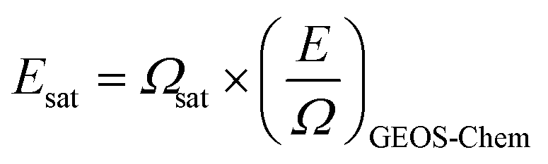Ω_sat is monthly mean TROPOMI NO₂ or IASI NH₃ column densities and (E/Ω)_GEOS-Chem is the modelled ratio of 24 h monthly total NO_x or NH₃ emissions to column densities of NO₂ or NH₃ averaged during the satellite overpass (Section 2.4). This approach attributes all the discrepancy between the satellite observations and model to biomass burning, so eqn (3) is only used for gridboxes with >50% contribution of biomass burning to total emissions, according to GEOS-Chem (Section 2.3). We use modelled emissions and columns driven with inventories that yield best agreement with TROPOMI for NO_x and with IASI for NH₃.

Interpretation of the spatial distribution of the emissions calculated with eqn (3) is aided by the global 0.5° pyrome classification dataset⁵⁹ archived by the Archibald Ecology Laboratory (https://archibaldlab.weebly.com/datasets.html, last accessed 25 February 2025) (Fig. S1†). Pyromes are classed by frequency, intensity, and size from Bayesian clustering informed by datasets of active fires, burned area, fire radiative power, fire season, ecoregions, and variables of climate and human influence.

3. Results

3.1 Bottom-up biomass burning NO_x and NH₃ emissions

Fig. 1 compares monthly June–October NO_x and NH₃ emissions from the three inventories. NO_x emissions totals are similar for GFEDv4s (4.5 Tg NO) and FINNv2.5 (4.8 Tg NO) and about 3-times less for GFASv1.2 (1.6 Tg NO). NH₃ emissions totals are similar for GFEDv4s (0.72 Tg) and GFASv1.2 (0.55 Tg) and at least double for FINNv2.5 at 1.4 Tg. Emissions peak in July according to GFEDv4s and GFASv1.2, and in August for FINNv2.5. Month-to-month variability is similar for GFEDv4s and GFASv1.2. FINNv2.5 exhibits distinct and greater seasonal variability than the other two inventories. FINNv2.5 emissions increase from similar emissions to GFASv1.2 in June to 4-times more NO_x and 6-times more NH₃ in August and sustaining 2- to 5-times more NO_x and 4-times more NH₃ than the other inventories in October.

Fig. 1 Comparison of monthly biomass burning NO_x and NH₃ emissions. Panels compare subtropical southern Africa biomass burning emissions of NO_x (as NO) (a) and NH₃ (b) in 2019 from the inventories GFEDv4s (blue), FINNv2.5 (red), and GFASv1.2 (green) and from our top-down estimate (black; Section 3.4). Inset regular font values are inventory and top-down totals for June–October, except for top-down NH₃ that is for July–October (time period shaded grey). Italicized values in parentheses are bottom-up NH₃ for July–October only.

Both dry matter burned and the choice of emission factors (Table 1) contribute to systematic differences in NO_x emissions between GFEDv4s and GFASv2.1. GFEDv4s uses a savanna emission factor (3.9 g NO_x as NO (kg DMB)⁻¹) that is almost double GFASv1.2 (2.1 g NO_x as NO (kg DMB)⁻¹). The effect of greater burned area in GFEDv4s is evident from differences in NH₃ emissions. The ∼40% greater emission factors for GFASv1.2 (0.74 g (kg DMB)⁻¹) than GFEDv4s (0.52 g (kg DMB)⁻¹) is offset by more dry matter burned in GFEDv4s. FINNv2.5 uses the same NO_x emission factor as GFEDv4s for savannas, and the chapparal vegetation type emission factor of 3.65 g NO_x as NO (kg DMB)⁻¹ for woody savannas that is similar to that for savannas, so differences between these two inventories is mostly due to estimated dry matter burned and more intense equatorward tropical forest fires in FINNv2.5. The forest fire emission factor in FINNv2.5 (2.5 g NO_x as NO (kg DMB)⁻¹) is less than the savanna emission factors, but the fuel consumed is far greater in FINNv2.5. FINNv2.5 burn fractions (α in eqn (2)) of 0.9 for savannas and 0.3 for tropical forests⁴⁰ and southern Africa fuel loads (B in eqn (2)) of 411 g m⁻² for savannas and 25 295 g m⁻² for tropical forests³⁶ amounts to ∼20-times more fuel consumed for tropical forests than savannas.

Distinct FINNv2.5 NH₃ emissions is in part because 20–30% of gridboxes with active fires are classified as woody savanna that has an emission factor (1.2 g (kg DMB)⁻¹) that is more than double that for savannas (Table 1). The proportion of woody savanna gridboxes in FINNv2.5 increases from ∼20% in June to ∼30% in August and declines back to ∼20% in October. Sustained October emissions in FINNv2.5 is because of widespread emissions in Angola and southwest Zambia that are either absent or far less intense in the other inventories.

Addition of VIIRS in FINNv2.5 increases total regional June–October NH₃ and NO_x emissions by ∼20% relative to emissions obtained with MODIS only. The effect on spatial coverage of emissions is small. Emissions using both VIIRS and MODIS sensors results in >600 000 more 0.1° daily gridboxes with emissions than the emissions product that uses MODIS only. Though this is a cumulative area of >700 000 km², the additional VIIRS gridboxes only amounts to 143 kt more NO_x as NO or just 3% of the Fig. 1(a) total. The increase in NH₃ emissions for these additional gridboxes is slightly more, at 8% (114 kt) of the Fig. 1(b) total.

In June–September, biomass burning dominates total boundary layer (<2 km) NO_x emissions in subtropical southern Africa, according to GEOS-Chem using GFEDv4s (monthly emissions range is 79–87% of total NO_x emissions), FINNv2.5 (72–87%), and GFASv1.2 (58–70%). The other prominent source is soil NO_x, totalling 110–190 kt NO or ∼10–30% of boundary layer NO_x emissions. By October, soil NO_x emissions of 200 kt NO are 86 kt more than GFASv1.2, 71 kt less than GFEDv4s, and less than half the 550 kt NO from FINNv2.5. Monthly anthropogenic NO_x, mostly from combustion of vehicular fuels and domestic burning of biomass and charcoal,^55,60,61 is a much smaller NO_x source than biomass burning and soils at 41–43 kt NO in June–October. Lightning is another prominent NO_x source in the region, but most (>95%) is emitted above the boundary layer, increasing from 28 kt NO in June to 140 kt NO in October with the transition to the rainy season.

For NH₃, the biomass burning contribution to total emissions is similar in June–September for GFEDv4s (40–52%) and GFASv1.2 (32–46%), but declines to 17–18% in October. For FINNv2.5, the contribution increases from 35% in June to 46–74% in July–October. The other major NH₃ source is anthropogenic, totalling 170–180 kt in each month from activities such as agriculture and charcoal production in rural areas and from vehicles and domestic burning of waste, biomass, and charcoal in urban areas.^55,60,61 More than half (∼53%) of this anthropogenic NH₃ is concentrated north of 5°S. Monthly natural NH₃ emissions total 19–21 kt.

A new GFED version (GFEDv5) has been developed that is undergoing quality checks and validation before final release (https://www.globalfiredata.org/data.html; last accessed 12 May 2025). GFEDv5 updates emission factors to the latest Binte Shahid et al.,²⁴ resulting in emissions for June–October that are 1.2 Tg more than GFEDv4s for NO_x at 5.7 Tg NO and ∼0.5 Tg more than GFEDv4s for NH₃ at 1.2 Tg. The NH₃ emissions seasonality shifts to a more pronounced August peak of 0.35 Tg for GFEDv5 compared to <0.2 Tg for GFEDv4s (Fig. 1(b)).

3.2 Evaluation of bottom-up NO_x emissions with TROPOMI NO₂ and implications for ozone and PAN

Fig. 2 compares TROPOMI and GEOS-Chem tropospheric NO₂ column densities averaged over June–October. Modelled NO₂ obtained with GFEDv4s and GFASv1.2 is more spatially consistent with TROPOMI (R = 0.93 for both) than FINNv2.5 (R = 0.64). The correlation in individual months exceeds 0.82 for GFEDv4s and GFASv1.2 and ranges from R = 0.42 in July to R = 0.75 in October for FINNv2.5. GEOS-Chem seasonal domain mean NO₂ is most consistent with TROPOMI using FINNv2.5 (NMB = 14%) and GFASv1.2 (NMB = −21%) compared to GFEDv4s (NMB = 44%). Due to large monthly variability in FINNv2.5 and GFEDv4s emissions (Fig. 1(a)), NMBs range from 2% in September to 50% in August for FINNv2.5 and from 1% in October to 75% in July for GFEDv4s. Those for GFASv1.2 are least variable at −14% in July to −28% in September. In June–September, FINNv2.5 NO_x emissions in the northern portion of the domain (pink dashed circles in Fig. 2) far exceed the other inventories. The northly extent of emissions in FINNv2.5 is in both the combined VIIRS and MODIS and the MODIS-only product and is because landcover there is tropical forest that, according to FINNv2.5, has 20-times greater fuel consumption than savannas.³⁶

Fig. 2 Observed vs. modelled June–October mean tropospheric column densities of NO₂. Panels are gridded (0.25° × 0.3125°) 2019 TROPOMI observations (a) and coincident GEOS-Chem using GFEDv4s (b), FINNv2.5 (c), and GFASv1.2 (d) all with TROPOMI averaging kernels applied (Section 2.4; Text S1†). Inset values in (b)–(d) are Pearson's correlation coefficients (R) and the model normalized mean bias (NMB) for the domain plotted. Countries discussed in Section 3.2 are indicated in (d) (DRC = Democratic Republic of the Congo, MOZ = Mozambique, MWI = Malawi, ZMB = Zambia). Pink dashed circles in all panels collocate the NO₂ hotspot from tropical forest fires discussed in the text.

The model overestimate in the integrated tropospheric column densities of NO₂ using GFEDv4s (Fig. 2(b)) is also apparent in comparisons of GEOS-Chem to discrete vertical profiles of free tropospheric NO₂ obtained by cloud-slicing total columns of TROPOMI NO₂. In that comparison, the model driven with GFEDv4s is more than double the June–August mean cloud-sliced NO₂ mixing ratios at 800–600 hPa (∼2–4 km) over southern Africa.⁶²

The averaging kernels applied to GEOS-Chem (Section 2.4; Text S1†) alter most monthly mean model gridboxes by ∼10%, with the exception of a few gridboxes in the DRC with larger enhancements in NO₂ (>5 × 10¹⁵ molecules cm⁻²) due to fires. These decline by 1–2 × 10¹⁵ molecules cm⁻² or 20–30%, due to the relatively poor sensitivity of TROPOMI to the lower troposphere.⁶³ The largest decline of 5–10 × 10¹⁵ molecules cm⁻² (25–65% decrease) is in August for NO₂ > 15 × 10¹⁵ molecules cm⁻² in central DRC obtained with GEOS-Chem using FINNv2.5.

A striking feature in Fig. 2(a)–(c) is the much lower NO₂ concentrations in Malawi than its neighbours Zambia and Mozambique. Malawi is amongst the least fire-prone countries in southern Africa, whereas its neighbours Zambia and Mozambique are amongst the most, based on 8 years of burned area data.⁶⁴ Malawi's mostly rural population density is ∼220 people km⁻², far more than its neighbours (<50 people km⁻²) (https://data.worldbank.org/indicator/EN.POP.DNST, last accessed 5 March 2025). There is a steep, exponential decline in fire size with population density.¹² A greater population density increases fire occurrence, but it also fragments the land, preventing fires that reach Malawi from propagating.^12,64

Differences in the NO_x emissions in Fig. 1(a) affect chemical production of ozone and PAN. According to GEOS-Chem, total chemical production of boundary layer ozone (O₃) in June–October is 20 Tg using GFASv1.2 that emits less NO_x than the other inventories (Fig. 1(a)). Ozone production with the other inventories is 11 Tg more than GFASv1.2 using GFEDv4s and 26 Tg more using FINNv2.5. Even though GFEDv4s and FINNv2.5 yield greater ozone production than GFASv1.2, the ozone production efficiency (OPE) for GFASv1.2 exceeds the other inventories. OPE for GFASv1.2 is 13 Tg O₃ (Tg NO)⁻¹ compared to 6.9 Tg O₃ (Tg NO)⁻¹ for GFEDv4s and 9.6 Tg O₃ (Tg NO)⁻¹ for FINNv2.5. Far more of the other ozone precursors, CO and non-methane volatile organic compounds (NMVOCs), in FINNv2.5 cause the greater OPE than GFEDv4s. FINNv2.5 emissions total 108 Tg CO and 13 Tg C for 21 NMVOCs compared to 82 Tg CO and 2.0 Tg C for 13 NMVOCs for GFEDv4s and 49 Tg CO and 0.82 Tg C for 12 NMVOCs for GFASv1.2. If all NO_x in FINNv2.5 is emitted as NO rather than mostly NO₂ (Section 2.1; Table 1), the OPE declines to 9.1 Tg O₃ (Tg NO)⁻¹, as there is more NO to react directly with ozone.

Boundary layer PAN is also affected by differences in NO_x emissions. PAN production with FINNv2.5 totals 3.6 Tg for June–October. This far exceeds the other inventories by 2.7 Tg for GFEDv4s and 3.1 Tg for GFASv1.2. In addition to differences in NO_x emissions, FINNv2.5 also includes NMVOCs with large PAN yields that are absent in the other inventories. Specifically, methyl glyoxal, methyl vinyl ketone, methacrolein, and hydroxyacetone.⁶⁵ PAN production efficiencies are 0.8 Tg PAN (Tg NO)⁻¹ for FINNv2.5, 0.2 Tg PAN (Tg NO)⁻¹ for GFEDv4s and 0.3 Tg PAN (Tg NO)⁻¹ for GFASv1.2. If all FINNv2.5 NO_x is emitted as NO, PAN production only declines by 0.1 Tg.

3.3 Evaluation of bottom-up NH₃ emissions with IASI

Fig. 3 compares NH₃ columns from the reprocessed IASI data and from GEOS-Chem for July–October. Even though we use IASI NH₃ from both MetOp-A and -B, data density is 20 to 24 times less than TROPOMI, due to the coarser IASI pixel resolution (Section 2.1). All three reprocessed products are very similar to each other, so differences relative to FINNv2.5 are shown for GFEDv4s (Fig. 3(b)) and GFASv1.2 (Fig. 3(c)). The spatial correlation (R) between products for individual months exceeds 0.95 and the relative difference in domain mean IASI NH₃ is <10%. More NH₃ emissions from FINNv2.5 compared to the other inventories (Fig. 1(b)) causes greater column densities in the DRC in the northcentral portion of the model domain. These are about 3–4 × 10¹⁵ molecules cm⁻² more in FINNv2.5, but the NH₃ columns there are still less prominent than the NH₃ due south in southern DRC. The model profile shape rather than magnitude is used in the retrieval, so there is limited influence of the prior on the spatial distribution of NH₃, as is evident in the distinct spatial distribution of NH₃ for the reprocessed IASI columns in Fig. 3(a) and the prior (Fig. 3(d)).

Fig. 3 Comparison of IASI and GEOS-Chem July–October mean NH₃. All gridded (0.25° × 0.3125°) maps are for 2019. Panels are IASI NH₃ retrieved with GEOS-Chem priors obtained using FINNv2.5 (a), the difference between (a) and IASI reprocessed with GEOS-Chem using GFEDv4s (b) and GFASv1.2 (c), and the GEOS-Chem IASI NH₃ columns obtained with FINNv2.5 (d), GFEDv4s (e) and GFASv1.2 (f). Grey grids mostly over the Atlantic Ocean lack at least 10 IASI pixels in all months (Text S2†). Values in (d)–(f) are Pearson's correlation coefficients (R) between IASI and the model and the model normalized mean bias (NMB) for the domain plotted. Countries discussed in Section 3.3 are indicated in (b) (AGO = Angola, DRC = Democratic Republic of the Congo, ZMB = Zambia). Pink dashed boxes in (a) identify features in Angola to the south and the Ukerewe basin in the north discussed in the text.

Replacing the default prior with GEOS-Chem leads to a systematic, extensive decrease in NH₃ column densities (Fig. S2†), as more NH₃ is distributed to higher altitudes in GEOS-Chem than the default terrestrial a priori profile. This was also the case for IASI PAN reprocessed with GEOS-Chem priors.⁵⁸ Specific NH₃ enhancements in the provided product that decrease on reprocessing include a persistent NH₃ enhancement along the west coast of Angola of 17–30 × 10¹⁵ molecules cm⁻² that declines to <15 × 10¹⁵ molecules cm⁻² with GEOS-Chem, and a decrease in the intensity of NH₃ in the Ukerewe (Lake Victoria) basin. The Ukerewe basin enhancement still occurs in the reprocessed product (pink dashed box in Fig. 3(a)) and is likely associated with anthropogenic activity, as this is one of the most densely populated, predominantly rural, regions in Africa.^66,67 The reprocessed NH₃ also has smoother spatial gradients than the provided product, such as along coastlines where the provided product a priori transitions from a fixed ocean to a fixed land vertical NH₃ profile. Fewer retrieved pixels are also removed in the postfilter step (Section 2.4) with GEOS-Chem as prior.

June is not in Fig. 3, as the spatial correlation is poor for all inventories (R < 0.5). The correlation improves to R = 0.62–0.83 in July–September and, in October, is stronger for FINNv2.5 (R = 0.70) than the other inventories (R = 0.38 for both). The major biomass burning NH₃ enhancement in the reprocessed IASI NH₃ in June that GEOS-Chem does not reproduce is fires in Angola. These include a widespread enhancement in NH₃ south of central Angola and a smaller, more intense well-defined plume along the border with Zambia, also apparent in July–October (Fig. 3(a)). This feature is absent in non-biomass burning months (Fig. S3†) and TROPOMI NO₂ is only marginally enhanced (<2.5 × 10¹⁵ molecules cm⁻²) in June over southern Angola, suggestive this is smouldering burning undetected by MODIS or VIIRS. Predominance of smouldering fires in June is consistent with the low combustion efficiency estimated by Fang et al.²² using satellite observations of CO and an assimilated CO₂ product. They attributed low combustion efficiency in June to relatively high fuel moisture content at the end of the rainy season.

Model NMBs for individual months are consistently biased high (NMB = 13–45%) in July and almost all biased low in August–October (NMB of −2% to −63%), except for FINNv2.5 that has a positive bias of 12% in August when its emissions far exceed the other inventories (Fig. 1(b)).

3.4 Top-down biomass burning NO_x and NH₃ emissions

We infer 24 h monthly NO_x and NH₃ emissions using eqn (3) (Section 2.5) and modelled emissions and columns driven with GFASv1.2 for NO_x, as it is most consistent with TROPOMI (Fig. 2), and FINNv2.5 for NH₃ for the same reason (Fig. 3). Emissions are also only estimated for months when GEOS-Chem and the satellite data are spatially correlated. These are June–October for NO_x (R = 0.85–0.94) and July–October for NH₃ (R = 0.68–0.81). According to the bottom-up inventories, model gridboxes with >50% biomass burning contribution to total emissions account for 93% of total biomass burning emissions for NO_x and 94% for NH₃.

Fig. 4 compares maps of collocated multi-month total top-down and bottom-up emissions of NO_x and NH₃. Top-down June–October NO_x emissions total 1.9 Tg compared to 1.5 Tg from GFASv1.2, due to widespread increases in emissions almost everywhere except northern Angola and southeast DRC. Top-down July–October NH₃ emissions total 1.2 Tg. This is only 27 kt less than FINNv2.5, as regional decline in top-down emissions in most of the west is balanced by increases in the east and in southern Angola. NO_x emissions across the domain are distributed normally (mean = 0.39 kt, median = 0.36 kt), whereas NH₃ has a long tail distribution (mean = 0.27 kt, median = 0.14 kt). Bottom-up and top-down emissions are very spatially consistent (R = 0.88 for NO_x, R = 0.89 for NH₃), as expected from selection of these inventories from comparison to TROPOMI and IASI (Fig. 2 and 3).

Fig. 4 Comparison of top-down and bottom-up reactive nitrogen emissions. Panels are top-down NO_x (a) and NH₃ (b), bottom-up GFASv1.2 NO_x (c) and FINNv2.5 NH₃ (d), and the difference between top-down and bottom-up NO_x (e) and NH₃ (f). Grey gridboxes have <50% biomass burning contribution to total emissions in all months, according to GEOS-Chem (Section 2.3). Arrows in (a) and (b) point to grey omitted gridboxes in and neighbouring Kinshasa discussed in Section 4. Inset values in (a)–(d) are emissions totals for NO_x in June–October and NH₃ in July–October. Top-down emissions totals for individual months are in Fig. 1. Countries discussed in Section 3.4 are indicated in (c) (AGO = Angola, DRC = Democratic Republic of the Congo, MOZ = Mozambique, MWI = Malawi, ZMB = Zambia).

NO_x emissions in northern Angola and southern DRC collocate with the yellow boomerang-shaped pyrome (Fig. S1†) of frequent, intense and large (FIL) fires that preferentially undergo flaming combustion. This is similarly the case for NO_x emissions in northeast Zambia and southeast Angola. The NO_x hotspot along the Angola/DRC border and also coincident with FIL fires is more pronounced in the top-down than the bottom-up emissions (Fig. 4(a) versus (c)), as expected from the relatively large TROPOMI tropospheric NO₂ column abundances in this location (Fig. 2(a)).

Many of the intense NH₃ emissions in Fig. 4(b) are spatially distinct from the intense NO_x emissions, except for those in Mozambique due south of Malawi. The correlation between top-down NO_x and NH₃ emissions in individual months is <0.4. Similarly, GFASv1.2 NO_x and FINNv2.5 NH₃ emissions are weakly correlated (also R < 0.4). The spatial consistency between NO_x and NH₃ emissions is much greater for each inventory (R > 0.99 for GFASv1.2, R > 0.87 for FINNv2.5).

Exclusive NH₃ emissions in the DRC coincide with fires classified as cool and small (Fig. S1†), so are more prone to smouldering, favouring formation of NH₃ over NO_x. These cool and small fires decline in frequency from occurring often to intermediate to rare with northerly extent. Both top-down and bottom-up NH₃ emissions extend further north into the Congolese forest than the pyrome regime map, likely because of encroachment of fires since the pyrome classification data record end date of 2010. Multiple independent studies corroborate a steep, statistically significant increase in fires at the southern edge of the Congolese forest^68–70 attributed to warmer, drier conditions.⁶⁸ Over the decade from the end of the pyrome classification time period (2010) to the observation record used here (2019), fires have increased by >50 active fires per 0.25° (∼28 km resolution) gridbox, based on trends in MODIS active fires.⁶⁹

Monthly top-down emissions totals are also shown in Fig. 1 for comparison to the bottom-up values. Top-down NO_x emissions shift the emissions peak from July in GFASv1.2 to August, though the top-down emissions estimate for July and August only differs by 19 kt. The top-down NO_x emissions suggest fires in subtropical southern Africa produce ∼25 Tg boundary layer ozone, based on an OPE of 13 Tg O₃ (Tg NO)⁻¹ obtained with GEOS-Chem using GFASv1.2 NO_x emissions (Section 3.2) and assuming linearity across the 0.4 Tg difference between the top-down and bottom-up NO_x emissions. Top-down NH₃ emissions are less than FINNv2.5 in all months (by 79 kt in July, 59 kt in August, and 9 kt in September), except October that is 120 kt more than FINNv2.5. Emissions peak in August for both estimates, though the top-down peak is less pronounced than FINNv2.5.

If GFEDv4s or FINNv2.5 instead of GFASv1.2 is used to estimate NO_x emissions, June–October totals are 2.2 Tg NO using GFEDv4s and 2.4 Tg NO using FINNv2.5 (Fig. S4(a)†). This is only 0.3–0.5 Tg more than the top-down emissions derived with GFASv1.2 and far more consistent than the 3.2 Tg NO spread in bottom-up emissions (Fig. 1(a)). All top-down estimates also peak in August and there is a substantial (∼1 Tg) decrease in the prominence of the FINNv2.5 August peak. Remaining differences in top-down NO_x emissions likely result from errors in free tropospheric NO₂ (ref. 71) where TROPOMI is most sensitive to NO₂.

If, for NH₃, GFEDv4s or GFASv1.2 is used to calculate top-down emissions, July–October totals are 0.9 Tg using GFEDv4s and 0.6 Tg using GFASv1.2 (Fig. S4(b)†). The values converge on a 0.6 Tg difference for top-down compared to 0.9 Tg difference for bottom-up. A large portion (∼0.2 Tg) of this spread is because many of the northerly equatorward forest fire emitting gridboxes in FINNv2.5 are absent in GFEDv4s and GFASv1.2, so the GEOS-Chem term in eqn (3) is zero for these gridboxes. Top-down emissions using GFEDv4s and GFASv1.2 shift the peak from July to August, but neither is as pronounced as FINNv2.5 (Fig. S4(b)†).

3.5 Error analysis of the top-down emissions

Potential sources of uncertainty in the top-down emissions include the satellite observations, the GEOS-Chem term in eqn (3), and GEOS-Chem inventories used to identify gridboxes with >50% contribution from biomass burning.

According to past error estimates for TROPOMI NO₂, the error is typically ∼30% and is dominated by the air mass factor used to convert slant columns to vertical column densities.⁴⁵ The IASI NH₃ relative error for the version 4 product we use is 19–36%.³³ These error estimates are for individual observations, so the random component decreases substantially by averaging over multiple months.

We quantify GEOS-Chem error contributions from emissions perturbation simulations. For the GEOS-Chem term in eqn (3), we assess the percent change in top-down emissions due to a perturbation in biomass burning emissions informed by differences between top-down and the selected bottom-up inventories in Fig. 1. Perturbation simulations are for August when emissions in NH₃ and NO_x peak. GFASv1.2 NO_x emissions are increased by 20% and FINNv2.5 NH₃ emissions are reduced by 12%. The domain mean change in top-down emissions for the same gridboxes shown in Fig. 4 is a ∼3% increase in NO_x emissions and a ∼2% decline in NH₃ emissions. The small change in emissions is because the perturbation in emissions causes a near-equal response in the column, as has been reported previously for top-down estimate of UK agricultural NH₃ emissions.⁵⁰

Bottom-up inventories of anthropogenic emissions are very uncertain and could impart errors in identifying gridboxes with >50% contribution from biomass burning. For NO_x, we test sensitivity to this by doubling anthropogenic NO_x emissions, prompted by the suggestion that these are underestimated in urban areas from a study that evaluated bottom-up emissions against single point measurements in 3 urban areas in Angola and 1 urban area in Zambia.⁷² For NH₃, informed by our own comparison of IASI and GEOS-Chem (Fig. 3), we halve anthropogenic NH₃ emissions, as the model overestimates NH₃ column densities over the densely populated Ukerewe basin (Section 3.3). The resultant biomass burning season (June–October for NO_x, July–October for NH₃) emissions are only 1% (25 kt NO) less than in Fig. 4(a) for NO_x and 3% (34 kt) more than Fig. 4(b) for NH₃. The limited sensitivity to biases in anthropogenic emissions is because these emissions are in populated areas where fire propagation is supressed.¹²

Conservatively, relative error contributions for NO_x emissions are 0.3 for TROPOMI, 0.03 for the GEOS-Chem term in eqn (3), and 0.01 for anthropogenic NO_x emissions. Adding these in quadrature yields total NO_x emissions of 1.9 ± 0.6 Tg. Similarly, for NH₃, contributions are at most 0.36 for IASI, 0.02 for the GEOS-Chem term in eqn (3), and 0.03 for anthropogenic NH₃ emissions. Domain total NH₃ emissions are then 1.2 ± 0.4 Tg.

4. Discussion

None of the inventories include primary sulfate and nitrate aerosol emissions. As a result, GEOS-Chem may overestimate NH₃ columns, due to an underestimate in partitioning of semi-volatile NH₃ to these acidic aerosols to form ammonium aerosol. We test sensitivity of modelled NH₃ to inclusion of primary sulfate and nitrate emissions by adding these to FINNv2.5, given its greater consistency with IASI (Fig. 3(e)). For simplicity, we allocate tropical forest sulfate and nitrate emission factors to fires north of 5°S and west of 30°E and savanna sulfate and nitrate emission factors to all other fires. The emission factors we use (per kg DMB) are 130 mg sulfate and 110 mg nitrate for tropical forests and 18 mg sulfate and 16 mg nitrate for savannas and woody savannas.²⁵ No emission factors are given for the chapparal landcover type used in FINNv2.5 for woody savannas (Section 3.1). The effect on the modelled NH₃ columns is near-negligible. With primary sulfate and nitrate, the model correlation is unchanged and the model NMB is only 1 percentage point less than in Fig. 3(d).

GFASv1.2 is the only inventory with recommended injection heights (Section 2.1). Emissions injected above the boundary layer would affect the comparisons in Fig. 2 and 3, due to variability in vertical sensitivity of the two instruments (Section 2.4). The GFASv1.2 injection heights in subtropical southern Africa typically extend to ∼3 km, but most (∼80%) emissions are released to the lowest 5 layers of the model, reaching 750–850 m above ground level. This is well within the daytime boundary layer when most biomass is burned (Section 2.1). Turning this injection height feature off in GEOS-Chem has no effect on the comparison statistics for NO₂ in Fig. 2(d) and NH₃ in Fig. 3(d), as GEOS-Chem immediately mixes surface layer emissions throughout the boundary layer.⁷³

There are more complex and computationally intensive approaches than eqn (3) to infer emissions from satellite observations. Some explicitly account for effects like non-linear chemistry and displacement of the observed trace gas from the emission gridbox or so-called smearing.^30,74 Such approaches are suitable for static perennial or seasonal sources, like anthropogenic or biogenic (vegetation) emissions, but are not practical for episodic biomass burning emissions. Another option is iteration that would account for non-linear chemistry and model errors in the amount and vertical distribution of free tropospheric NO₂. The top-down emissions obtained in our study would be embedded in the model or used to scale the prior emissions to simulate top-down-informed columns that would then be used to obtain new top-down emissions. This process would be repeated until a pre-defined convergence criterion is met,⁷⁵ but such an approach is computationally costly. Another inversion approach is application of wind rotation and a plume fitting model to TROPOMI NO₂ to estimate NO_x emissions of individual fire plumes.⁷⁶ This method has been successfully applied to individual fires in Africa using daily TROPOMI observations, but it only yields top-down emissions for select isolated plumes with a well-defined Gaussian shape on wind rotation.⁷⁷ Even so, the plume NO_x emissions that were derived exhibit a strong linear relationship with fire radiative power⁷⁷ that we also find is a suitable explanatory variable for NO_x emissions (Section 3.2).

Our top-down emissions would ideally be validated by simulating GEOS-Chem with these top-down emissions and comparing modelled concentrations to independent ground-based observations of NO_x and NH₃. The long-term International Network to Study Deposition and Atmospheric composition in Africa (INDAAF) designed to monitor dry and wet deposition includes trace gas surface concentration measurements of NH₃ and NO₂, but all are located outside the latitude band considered here.⁷⁸ The recent intensive (January 2019) Methane Observations and Yearly Assessments (MOYA) aircraft campaign sampled biomass burning plumes over Uganda, but these were for the northern hemisphere burning season and limited to CO and long-lived greenhouse gases.⁷⁹ There are routine commercial aircraft observations from the In-service Aircraft for a Global Observing System (IAGOS) programme, but these flights sample the vertical distribution of the troposphere at airports dominated by anthropogenic pollution or influenced by long-range transported biomass burning plumes.⁷

Validation of the satellite observations for conditions relevant to this work is also not feasible. There was a ground-based Multi-Axis Differential Optical Absorption Spectroscopy (MAX-DOAS) instrument measuring vertical column densities of NO₂ in Burundi for assessment of space-based tropospheric columns of NO₂,⁸⁰ but it ceased operating before TROPOMI launched and would anyway have been mostly influenced by anthropogenic emissions from the densely populated Ukerewe basin. A MAX-DOAS instrument has been operating in the fast-growing capital city of the DRC, Kinshasa, since 2019,⁸¹ but data over this city are excluded in the top-down inference of emissions (arrows in Fig. 4(a) and (b)), as emissions are mostly from non-biomass burning sources. Optimum locations of ground-based instruments to validate satellite observations of biomass burning NO₂ and NH₃ are national parks where burning is intense and propagates over large areas.¹²

Our results suggest that the most suitable approach to estimate byproducts of flaming fires is to use either burned area or fire radiative power products with a savanna NO_x emission factor of 2.1 g (kg DMB)⁻¹. Though this NO_x emission factor is unpublished, it is similar to the mean value of 2.4 g (kg DMB)⁻¹ reported by Andreae.²⁶ Other byproducts that would similarly be produced in relative abundance with these fires include black carbon and carbon dioxide (CO₂).

For smouldering fire emissions, the most suitable approach is application of landscape-specific fuel loadings and burning completeness fractions to active fires and NH₃ emission factors that distinguish landcover by the relative coverage of woody vegetation, as in FINNv2.5. Co-emitted smouldering fire byproducts include CO, organic aerosols, methane, and NMVOCs. The distinct August peak in NH₃ emissions in Fig. 1(b) is corroborated by top-down estimates of CO emissions for southern Africa from inversion of satellite observations of CO²¹ and from bottom-up emissions estimates using the very high spatial resolution (20 m) Sentinel-2 instrument for enhanced detection of small fires.⁸² The top-down CO emissions from Zheng et al.²¹ are 1.5 to 2 times more than CO from GFASv1.2 and GFEDv4s in August–October. Combustion efficiency, determined as the ratio of CO₂ to the sum of CO and CO₂, also declines from ∼0.93 in May–July to 0.84–0.87 in August–October due to an increase in fuel moisture content as the region transitions to the rainy season.²¹

The GFASv1.2 spatial consistency with TROPOMI NO₂ would likely also occur with the NASA Quick Fire Emissions Dataset (QFED) inventory that too is generated with fire radiative power (https://gmao.gsfc.nasa.gov/pubs/docs/Darmenov796.pdf). The next version of GFED (v5) would worsen the discrepancy with TROPOMI NO₂ in Fig. 2(b) and with the TROPOMI-derived NO_x emissions. GFEDv5 NH₃ emissions reproduce the IASI-derived domain total emissions (both 1.2 Tg) and would better match the top-down seasonality in Fig. 1(b) than GFEDv4s. Consistency with the spatial distribution of IASI NH₃ may remain an issue, as the distinct enhancement in NH₃ emissions in the southern edge of the Congolese forest in Fig. 4(b) is absent in GFEDv5.

5. Conclusions

We determined reactive nitrogen emissions of NO_x and NH₃ for the 2019 burning season in subtropical southern Africa using the GEOS-Chem model driven with three distinct biomass burning inventories (FINNv2.5, GFEDv4s, GFASv1.2) and satellite observations of NO₂ from TROPOMI and NH₃ from IASI. Mass balance top-down emissions estimates used GEOS-Chem driven with inventories yielding column density abundances with greatest spatial and regional mean consistency with TROPOMI (GFASv1.2) and with IASI (FINNv2.5).

Our top-down estimated biomass burning emissions total 1.9 ± 0.6 Tg NO_x as NO for June–October and 1.2 ± 0.4 Tg NH₃ for July–October. The satellite observations make the largest contribution to uncertainties in the emissions estimates. June is excluded for NH₃, due to poor agreement of GEOS-Chem with IASI using all three inventories. The model does not reproduce the IASI NH₃ enhancements in Angola that may be due to smouldering fires at the start of the burning season. The IASI observations suggest then that the burning season initiates in the southwest, upending current understanding that burning begins in the north and propagates south.

We find with GEOS-Chem sensitivity simulations that our top-down emissions estimates of NO_x and NH₃ are unaffected by including plume injection height, due to the relatively low altitude of fire plumes in this region, and that emissions of NH₃ are unchanged by inclusion of primary emissions of acidic sulfate and nitrate aerosols that promote partitioning of semi-volatile NH₃ to aerosols.

We additionally derive a top-down informed June–October ozone production efficiency (OPE) of 13 Tg O₃ (Tg NO)⁻¹. Far greater GFEDv4s (4.5 Tg NO) and FINNv2.5 (4.8 Tg NO) NO_x emissions than the top-down estimate decreases the OPE to 7–10 Tg O₃ (Tg NO)⁻¹ due to transition to a far less NO_x-sensitive O₃ production regime. PAN production is greatest with FINNv2.5, due to inclusion of high-yielding PAN precursor NMVOCs.

All inventories collocate NO_x and NH₃ emissions, whereas top-down estimates suggest these are distinct for almost all fires, supportive of a hybrid bottom-up approach. Such an inventory could apply landscape specific fuel loads and combustion completeness to active fires for smouldering emissions and burned area or fire radiative power data for flaming emissions. Still, the June southern Angola enhancement in NH₃ would be absent in this hybrid approach.

Data availability

Gridded 2D data generated for this article available for download from the UCL Data Repository include top-down monthly total biomass burning NO_x and NH₃ emissions (Fig. 4), monthly mean GEOS-Chem tropospheric columns of NO₂ co-sampled with TROPOMI (Fig. 2), total columns of NH₃ co-sampled with IASI (Fig. 3), and monthly mean IASI NH₃ columns reprocessed with GEOS-Chem a priori profiles (Fig. 3) [https://doi.org/10.5522/04/28712444].

Author contributions

Study concept, formal analysis, investigation, methodology, and original draft by EAM, data provision and guidance on use by MVD and LC for IASI, CW for FINNv2.5, GvdW for GFEDv5, and KM for GFASv1.2 implementation in GEOS-Chem. All authors contributed to editing and reviewing the manuscript.

Conflicts of interest

There are no conflicts to declare.

Acknowledgements

The authors are grateful for helpful discussions with pyrome data developer Sally Archibald and GFAS inventory developer Johannes Kaiser. EAM is grateful for support from the European Research Council under the European Union's Horizon 2020 research and innovation programme (through a Starting Grant awarded to Eloise A. Marais, UpTrop (grant no. 851854)). LC is a Senior Research Associate with the Fonds de la Recherche Scientifique – FNRS. MVD is supported by the FED-tWIN project ARENBERG (“Assessing the Reactive Nitrogen Budget and Emissions at Regional and Global Scales”) funded via the Belgian Science Policy Office (BELSPO).

References

1. D. A. Hegg, L. F. Radke, P. V. Hobbs and P. J. Riggan, Ammonia emissions from biomass burning, Geophys. Res. Lett., 1988, 15, 335–337.
2. P. J. Crutzen, L. E. Heidt, J. P. Krasnec, W. H. Pollock and W. Seiler, Biomass burning as a source of atmospheric gases CO, H₂, N₂O, NO, CH₃Cl and COS, Nature, 1979, 282, 253–256.
3. C. L. Heald, D. A. Ridley, J. H. Kroll, S. R. H. Barrett, K. E. Cady-Pereira, M. J. Alvarado and C. D. Holmes, Contrasting the direct radiative effect and direct radiative forcing of aerosols, Atmos. Chem. Phys., 2014, 14, 5513–5527.
4. F. Paulot, D. Paynter, P. Ginoux, V. Naik, S. Whitburn, M. Van Damme, L. Clarisse, P. F. Coheur and L. W. Horowitz, Gas-aerosol partitioning of ammonia in biomass burning plumes: Implications for the interpretation of spaceborne observations of ammonia and the radiative forcing of ammonium nitrate, Geophys. Res. Lett., 2017, 44, 8084–8093.
5. M. O. Andreae, in Biogeochemistry of Global Change, 1993, ch. 7, pp. 113–150,  DOI:10.1007/978-1-4615-2812-8_7.
6. V. Vakkari, J. P. Beukes, M. Josipovic and P. G. van Zyl, Observations of ozone formation in southern African savanna and grassland fire plumes, Atmos. Environ., 2020, 223, 117256.
7. B. Sauvage, V. Thouret, J. P. Cammas, F. Gheusi, G. Athier and P. Nédélec, Tropospheric ozone over Equatorial Africa: regional aspects from the MOZAIC data, Atmos. Chem. Phys., 2005, 5, 311–335.
8. K. Vohra, E. A. Marais, W. J. Bloss, J. Schwartz, L. J. Mickley, M. Van Damme, L. Clarisse and P.-F. Coheur, Rapid rise in premature mortality due to anthropogenic air pollution in fast-growing tropical cities from 2005 to 2018, Sci. Adv., 2022, 8, eabm4435.
9. G. R. van der Werf, J. T. Randerson, L. Giglio, T. T. van Leeuwen, Y. Chen, B. M. Rogers, M. Mu, M. J. E. van Marle, D. C. Morton, G. J. Collatz, R. J. Yokelson and P. S. Kasibhatla, Global fire emissions estimates during 1997–2016, Earth Syst. Sci. Data, 2017, 9, 697–720.
10. R. Ramo, E. Roteta, I. Bistinas, D. van Wees, A. Bastarrika, E. Chuvieco and G. R. van der Werf, African burned area and fire carbon emissions are strongly impacted by small fires undetected by coarse resolution satellite data, Proc. Natl. Acad. Sci. U. S. A., 2021, 118, e2011160118.
11. C. Ichoku, in Oxford Research Encyclopedia of Climate Science, 2020,  DOI:10.1093/acrefore/9780190228620.013.523.
12. S. Archibald, Managing the human component of fire regimes: lessons from Africa, Philos. Trans. R. Soc., B, 2016, 371, 20150346.
13. N. Andela and G. R. van der Werf, Recent trends in African fires driven by cropland expansion and El Niño to La Niña transition, Nat. Clim. Change, 2014, 4, 791–795.
14. B. Byrne, J. Liu, K. W. Bowman, M. Pascolini-Campbell, A. Chatterjee, S. Pandey, K. Miyazaki, G. R. van der Werf, D. Wunch, P. O. Wennberg, C. M. Roehl and S. Sinha, Carbon emissions from the 2023 Canadian wildfires, Nature, 2024, 633, 835–839.
15. I. R. van der Velde, G. R. van der Werf, S. Houweling, J. D. Maasakkers, T. Borsdorff, J. Landgraf, P. Tol, T. A. van Kempen, R. van Hees, R. Hoogeveen, J. P. Veefkind and I. Aben, Vast CO₂ release from Australian fires in 2019–2020 constrained by satellite, Nature, 2021, 597, 366–369.
16. S. N. Behera, M. Sharma, V. P. Aneja and R. Balasubramanian, Ammonia in the atmosphere: a review on emission sources, atmospheric chemistry and deposition on terrestrial bodies, Environ. Sci. Pollut. Res., 2013, 20, 8092–8131.
17. L. W. A. Chen, P. Verburg, A. Shackelford, D. Zhu, R. Susfalk, J. C. Chow and J. G. Watson, Moisture effects on carbon and nitrogen emission from burning of wildland biomass, Atmos. Chem. Phys., 2010, 10, 6617–6625.
18. J. M. Roberts, C. E. Stockwell, R. J. Yokelson, J. de Gouw, Y. Liu, V. Selimovic, A. R. Koss, K. Sekimoto, M. M. Coggon, B. Yuan, K. J. Zarzana, S. S. Brown, C. Santin, S. H. Doerr and C. Warneke, The nitrogen budget of laboratory-simulated western US wildfires during the FIREX 2016 Fire Lab study, Atmos. Chem. Phys., 2020, 20, 8807–8826.
19. I. R. van der Velde, G. R. van der Werf, S. Houweling, H. J. Eskes, J. P. Veefkind, T. Borsdorff and I. Aben, Biomass burning combustion efficiency observed from space using measurements of CO and NO₂ by the TROPOspheric Monitoring Instrument (TROPOMI), Atmos. Chem. Phys., 2021, 21, 597–616.
20. B. Mota and M. J. Wooster, A new top-down approach for directly estimating biomass burning emissions and fuel consumption rates and totals from geostationary satellite fire radiative power (FRP), Remote Sens. Environ., 2018, 206, 45–62.
21. B. Zheng, F. Chevallier, P. Ciais, Y. Yin and Y. Wang, On the role of the flaming to smoldering transition in the seasonal cycle of African fire emissions, Geophys. Res. Lett., 2018, 45, 11998–12007.
22. X. Fang, Z. Wang, X. Huang, L. Xue, W. Hua, S. Lou, K. Ding and A. Ding, Variation of Modified Combustion Efficiency and its impact on biomass burning emission estimation in Africa, J. Geophys. Res.: Atmos., 2024, 129, e2024JD041808.
23. M. O. Andreae and P. Merlet, Emission of trace gases and aerosols from biomass burning, Global Biogeochem. Cycles, 2001, 15, 955–966.
24. S. Binte Shahid, F. G. Lacey, C. Wiedinmyer, R. J. Yokelson and K. C. Barsanti, NEIVAv1.0: Next-generation Emissions InVentory expansion of Akagi et al. (2011) version 1.0, Geosci. Model Dev., 2024, 17, 7679–7711.
25. S. K. Akagi, R. J. Yokelson, C. Wiedinmyer, M. J. Alvarado, J. S. Reid, T. Karl, J. D. Crounse and P. O. Wennberg, Emission factors for open and domestic biomass burning for use in atmospheric models, Atmos. Chem. Phys., 2011, 11, 4039–4072.
26. M. O. Andreae, Emission of trace gases and aerosols from biomass burning – an updated assessment, Atmos. Chem. Phys., 2019, 19, 8523–8546.
27. A. K. Mebust and R. C. Cohen, Observations of a seasonal cycle in NO_x emissions from fires in African woody savannas, Geophys. Res. Lett., 2013, 40, 1451–1455.
28. R. J. Swap, H. J. Annegarn, J. T. Suttles, J. Haywood, M. C. Helmlinger, C. Hely, P. V. Hobbs, B. N. Holben, J. Ji, M. D. King, T. Landmann, W. Maenhaut, L. Otter, B. Pak, S. J. Piketh, S. Platnick, J. Privette, D. Roy, A. M. Thompson, D. Ward and R. Yokelson, The Southern African Regional Science Initiative (SAFARI 2000): Overview of the dry season field campaign, S. Afr. J. Sci., 2002, 98, 6.
29. R. A. Delmas, A. Druilhet, B. Cros, P. Durand, C. Delon, J. P. Lacaux, J. M. Brustet, D. Serça, C. Affre, A. Guenther, J. Greenberg, W. Baugh, P. Harley, L. Klinger, P. Ginoux, G. Brasseur, P. R. Zimmerman, J. M. Grégoire, E. Janodet, A. Tournier, P. Perros, T. Marion, A. Gaudichet, H. Cachier, S. Ruellan, P. Masclet, S. Cautenet, D. Poulet, C. B. Biona, D. Nganga, J. P. Tathy, A. Minga, J. Loemba-Ndembi and P. Ceccato, Experiment for Regional Sources and Sinks of Oxidants (EXPRESSO): An overview, J. Geophys. Res.: Atmos., 1999, 104, 30609–30624.
30. E. A. Marais, D. J. Jacob, T. P. Kurosu, K. Chance, J. G. Murphy, C. Reeves, G. Mills, S. Casadio, D. B. Millet, M. P. Barkley, F. Paulot and J. Mao, Isoprene emissions in Africa inferred from OMI observations of formaldehyde columns, Atmos. Chem. Phys., 2012, 12, 6219–6235.
31. D. M. Westervelt, P. K. Isevulambire, R. Yombo Phaka, L. H. Yang, G. Raheja, G. Milly, J.-L. B. Selenge, J. P. M. Mulumba, D. Bousiotis, B. L. Djibi, V. F. McNeill, N. L. Ng, F. Pope, G. K. Mbela and J. N. Konde, Low-cost investigation into sources of PM_2.5 in Kinshasa, Democratic Republic of the Congo, ACS ES&T Air, 2023, 1, 43–51.
32. E. Irankunda, Z. Török, A. Mereuţă, J. Gasore, E. Kalisa, B. Akimpaye, T. Habineza, O. Shyaka, G. Munyampundu and A. Ozunu, The comparison between in-situ monitored data and modelled results of nitrogen dioxide (NO₂): case-study, road networks of Kigali city, Rwanda, Heliyon, 2022, 8, e12390.
33. L. Clarisse, B. Franco, M. Van Damme, T. Di Gioacchino, J. Hadji-Lazaro, S. Whitburn, L. Noppen, D. Hurtmans, C. Clerbaux and P. Coheur, The IASI NH₃ version 4 product: averaging kernels and improved consistency, Atmos. Meas. Tech., 2023, 16, 5009–5028.
34. M. Van Damme, L. Clarisse, C. L. Heald, D. Hurtmans, Y. Ngadi, C. Clerbaux, A. J. Dolman, J. W. Erisman and P. F. Coheur, Global distributions, time series and error characterization of atmospheric ammonia (NH₃) from IASI satellite observations, Atmos. Chem. Phys., 2014, 14, 2905–2922.
35. K. Lange, A. Richter, A. Schönhardt, A. C. Meier, T. Bösch, A. Seyler, K. Krause, L. K. Behrens, F. Wittrock, A. Merlaud, F. Tack, C. Fayt, M. M. Friedrich, E. Dimitropoulou, M. Van Roozendael, V. Kumar, S. Donner, S. Dörner, B. Lauster, M. Razi, C. Borger, K. Uhlmannsiek, T. Wagner, T. Ruhtz, H. Eskes, B. Bohn, D. Santana Diaz, N. Abuhassan, D. Schüttemeyer and J. P. Burrows, Validation of Sentinel-5P TROPOMI tropospheric NO₂ products by comparison with NO₂ measurements from airborne imaging DOAS, ground-based stationary DOAS, and mobile car DOAS measurements during the S5P-VAL-DE-Ruhr campaign, Atmos. Meas. Tech., 2023, 16, 1357–1389.
36. C. Wiedinmyer, Y. Kimura, E. C. McDonald-Buller, L. K. Emmons, R. R. Buchholz, W. Tang, K. Seto, M. B. Joseph, K. C. Barsanti, A. G. Carlton and R. Yokelson, The Fire Inventory from NCAR version 2.5: an updated global fire emissions model for climate and chemistry applications, Geosci. Model Dev., 2023, 16, 3873–3891.
37. J. W. Kaiser, A. Heil, M. O. Andreae, A. Benedetti, N. Chubarova, L. Jones, J. J. Morcrette, M. Razinger, M. G. Schultz, M. Suttie and G. R. van der Werf, Biomass burning emissions estimated with a global fire assimilation system based on observed fire radiative power, Biogeosciences, 2012, 9, 527–554.
38. ECMWF, CAMS global biomass burning emissions based on fire radiative power (GFAS): data documentation, https://confluence.ecmwf.int/display/CKB/CAMS+global+biomass+burning+emissions+based+on+fire+radiative+power+%28GFAS%29%3A+data+documentation, accessed 9 January, 2025.
39. W. Seiler and P. J. Crutzen, Estimates of gross and net fluxes of carbon between the biosphere and the atmosphere from biomass burning, Clim. Change, 1980, 2, 207–247.
40. C. Wiedinmyer, S. K. Akagi, R. J. Yokelson, L. K. Emmons, J. A. Al-Saadi, J. J. Orlando and A. J. Soja, The Fire INventory from NCAR (FINN): A high resolution global model to estimate the emissions from open burning, Geosci. Model Dev., 2011, 4, 625–641.
41. M. Mu, J. T. Randerson, G. R. van der Werf, L. Giglio, P. Kasibhatla, D. Morton, G. J. Collatz, R. S. DeFries, E. J. Hyer, E. M. Prins, D. W. T. Griffith, D. Wunch, G. C. Toon, V. Sherlock and P. O. Wennberg, Daily and 3-hourly variability in global fire emissions and consequences for atmospheric model predictions of carbon monoxide, J. Geophys. Res.: Atmos., 2011, 116, D24303.
42. S. Rémy, A. Veira, R. Paugam, M. Sofiev, J. W. Kaiser, F. Marenco, S. P. Burton, A. Benedetti, R. J. Engelen, R. Ferrare and J. W. Hair, Two global data sets of daily fire emission injection heights since 2003, Atmos. Chem. Phys., 2017, 17, 2921–2942.
43. H. Eskes, J. van Geffen, M. Sneep, P. Veefkind, S. Niemeijer and C. Zehner, S5P Nitrogen Dioxide v02.03.01 intermediate reprocessing on the S5P-PAL system: Readme file, 2021.
44. H. Eskes, K.-U. Eichmann, J.-C. Lambert, D. Loyola, D. Stein-Zweers, A. Dehn and C. Zehner, ATM-MPC Mission Performance Cluster Nitrogen Dioxide [L2__NO2___] Readme, 2024.
45. J. van Geffen, H. Eskes, K. F. Boersma and P. Veefkind, TROPOMI ATBD of the Total and Tropospheric NO2 Data Products (Issue 2.2.0), Royal Netherlands Meteorological Institute (KNMI), De Bilt, The Netherlands, 2021.
46. Air-Sciences-Inc., 2002 Fire Emission Inventory for the WRAP Region – Phase II, Air Sciences Inc., 2005.
47. A. F. Bouwman, D. S. Lee, W. A. H. Asman, F. J. Dentener, K. W. Van Der Hoek and J. G. J. Olivier, A global high-resolution emission inventory for ammonia, Global Biogeochem. Cycles, 1997, 11, 561–587.
48. D. Simpson, W. Winiwarter, G. Börjesson, S. Cinderby, A. Ferreiro, A. Guenther, C. N. Hewitt, R. Janson, M. A. K. Khalil, S. Owen, T. E. Pierce, H. Puxbaum, M. Shearer, U. Skiba, R. Steinbrecher, L. Tarrasón and M. G. Öquist, Inventorying emissions from nature in Europe, J. Geophys. Res.: Atmos., 1999, 104, 8113–8152.
49. F. Paulot, D. J. Jacob, R. W. Pinder, J. O. Bash, K. Travis and D. K. Henze, Ammonia emissions in the United States, European Union, and China derived by high-resolution inversion of ammonium wet deposition data: Interpretation with a new agricultural emissions inventory (MASAGE_NH3), J. Geophys. Res.: Atmos., 2014, 119, 4343–4364.
50. E. A. Marais, A. K. Pandey, M. Van Damme, L. Clarisse, P. F. Coheur, M. W. Shephard, K. E. Cady-Pereira, T. Misselbrook, L. Zhu, G. Luo and F. Yu, UK ammonia emissions estimated With satellite observations and GEOS-Chem, J. Geophys. Res.: Atmos., 2021, 126, e2021JD035237.
51. L. T. Murray, D. J. Jacob, J. A. Logan, R. C. Hudman and W. J. Koshak, Optimized regional and interannual variability of lightning in a global chemical transport model constrained by LIS/OTD satellite data, J. Geophys. Res.: Atmos., 2012, 117, D20307.
52. R. C. Hudman, N. E. Moore, A. K. Mebust, R. V. Martin, A. R. Russell, L. C. Valin and R. C. Cohen, Steps towards a mechanistic model of global soil nitric oxide emissions: implementation and space based-constraints, Atmos. Chem. Phys., 2012, 12, 7779–7795.
53. R. M. Hoesly, S. J. Smith, L. Feng, Z. Klimont, G. Janssens-Maenhout, T. Pitkanen, J. J. Seibert, L. Vu, R. J. Andres, R. M. Bolt, T. C. Bond, L. Dawidowski, N. Kholod, J.-i. Kurokawa, M. Li, L. Liu, Z. Lu, M. C. P. Moura, P. R. O'Rourke and Q. Zhang, Historical (1750–2014) anthropogenic emissions of reactive gases and aerosols from the Community Emissions Data System (CEDS), Geosci. Model Dev., 2018, 11, 369–408.
54. E. E. McDuffie, S. J. Smith, P. O'Rourke, K. Tibrewal, C. Venkataraman, E. A. Marais, B. Zheng, M. Crippa, M. Brauer and R. V. Martin, A global anthropogenic emission inventory of atmospheric pollutants from sector- and fuel-specific sources (1970–2017): an application of the Community Emissions Data System (CEDS), Earth Syst. Sci. Data, 2020, 12, 3413–3442.
55. E. A. Marais and C. Wiedinmyer, Air Quality Impact of Diffuse and Inefficient Combustion Emissions in Africa (DICE-Africa), Environ. Sci. Technol., 2016, 50, 10739–10745.
56. C. Fountoukis and A. Nenes, ISORROPIA II: a computationally efficient thermodynamic equilibrium model for K⁺-Ca₂⁺-Mg₂⁺-NH₄⁺-Na⁺-SO₄^2--NO₃^--Cl^--H₂O aerosols, Atmos. Chem. Phys., 2007, 7, 4639–4659.
57. H. Eskes, J. v. Geffen, F. Boersma, K.-U. Eichmann, A. Apituley, M. Pedergnana, M. Sneep, J. P. Veefkind and D. Loyola, Sentinel-5 precursor/TROPOMI Level 2 Product User Manual Nitrogendioxide, 2022.
58. S. Zhai, D. J. Jacob, B. Franco, L. Clarisse, P. Coheur, V. Shah, K. H. Bates, H. Lin, R. Dang, M. P. Sulprizio, L. G. Huey, F. L. Moore, D. A. Jaffe and H. Liao, Transpacific transport of Asian peroxyacetyl nitrate (PAN) observed from satellite: Implications for ozone, Environ. Sci. Technol., 2024, 58, 9760–9769.
59. S. Archibald, C. E. R. Lehmann, J. L. Gómez-Dans and R. A. Bradstock, Defining pyromes and global syndromes of fire regimes, Proc. Natl. Acad. Sci. U. S. A., 2013, 110, 6442–6447.
60. A. S. Bockarie, E. A. Marais and A. R. MacKenzie, Air pollution and climate forcing of the charcoal industry in Africa, Environ. Sci. Technol., 2020, 54, 13429–13438.
61. S. Keita, C. Liousse, E.-M. Assamoi, T. Doumbia, E. T. N'Datchoh, S. Gnamien, N. Elguindi, C. Granier and V. Yoboué, African anthropogenic emissions inventory for gases and particles from 1990 to 2015, Earth Syst. Sci. Data, 2021, 13, 3691–3705.
62. R. P. Horner, E. A. Marais, N. Wei, R. G. Ryan and V. Shah, Vertical profiles of global tropospheric nitrogen dioxide (NO₂) obtained by cloud slicing the TROPOspheric Monitoring Instrument (TROPOMI), Atmos. Chem. Phys., 2024, 24, 13047–13064.
63. J. Douros, H. Eskes, J. van Geffen, K. F. Boersma, S. Compernolle, G. Pinardi, A.-M. Blechschmidt, V.-H. Peuch, A. Colette and P. Veefkind, Comparing Sentinel-5P TROPOMI NO₂ column observations with the CAMS regional air quality ensemble, Geosci. Model Dev., 2023, 16, 509–534.
64. S. Archibald, R. J. Scholes, D. P. Roy, G. Roberts and L. Boschetti, Southern African fire regimes as revealed by remote sensing, Int. J. Wildland Fire, 2010, 19, 861–878.
65. E. V. Fischer, D. J. Jacob, R. M. Yantosca, M. P. Sulprizio, D. B. Millet, J. Mao, F. Paulot, H. B. Singh, A. Roiger, L. Ries, R. W. Talbot, K. Dzepina and S. Pandey Deolal, Atmospheric peroxyacetyl nitrate (PAN): a global budget and source attribution, Atmos. Chem. Phys., 2014, 14, 2679–2698.
66. C. Nyamweya, T. J. Lawrence, M. Z. Ajode, S. Smith, A. O. Achieng, J. E. Barasa, F. O. Masese, A. Taabu-Munyaho, S. Mahongo, R. Kayanda, E. Rukunya, L. Kisaka, J. Manyala, M. Medard, S. Otoung, H. Mrosso, B. Sekadende, J. Walakira, S. Mbabazi, M. Kishe, A. Shoko, T. Dadi, A. Gemmell and W. Nkalubo, Lake Victoria: Overview of research needs and the way forward, J. Great Lakes Res., 2023, 49, 102211.
67. M. Olokotum, V. Mitroi, M. Troussellier, R. Semyalo, C. Bernard, B. Montuelle, W. Okello, C. Quiblier and J.-F. Humbert, A review of the socioecological causes and consequences of cyanobacterial blooms in Lake Victoria, Harmful Algae, 2020, 96, 101829.
68. Y. Jiang, L. Zhou and A. Raghavendra, Observed changes in fire patterns and possible drivers over Central Africa, Environ. Res. Lett., 2020, 15, 0940b8.
69. M. C. Wimberly, D. Wanyama, R. Doughty, H. Peiro and S. Crowell, Increasing fire activity in African tropical forests is associated with deforestation and climate change, Geophys. Res. Lett., 2024, 51, e2023GL106240.
70. A. C. Shapiro, H. S. Grantham, N. Aguilar-Amuchastegui, N. J. Murray, V. Gond, D. Bonfils and O. Rickenbach, Forest condition in the Congo Basin for the assessment of ecosystem conservation status, Ecol. Indic., 2021, 122, 107268.
71. R. F. Silvern, D. J. Jacob, L. J. Mickley, M. P. Sulprizio, K. R. Travis, E. A. Marais, R. C. Cohen, J. L. Laughner, S. Choi, J. Joiner and L. N. Lamsal, Using satellite observations of tropospheric NO₂ columns to infer long-term trends in US NO_x emissions: the importance of accounting for the free tropospheric NO₂ background, Atmos. Chem. Phys., 2019, 19, 8863–8878.
72. Y. Wang, K. Li, X. Chen, Z. Yang, M. Tang, P. M. D. Campos, Y. Yang, X. Yue and H. Liao, Revisiting the high tropospheric ozone over southern Africa: role of biomass burning and anthropogenic emissions, Atmos. Chem. Phys., 2025, 25, 4455–4475.
73. J.-T. Lin and M. B. McElroy, Impacts of boundary layer mixing on pollutant vertical profiles in the lower troposphere: Implications to satellite remote sensing, Atmos. Environ., 2010, 44, 1726–1739.
74. L. N. Lamsal, R. V. Martin, A. Padmanabhan, A. van Donkelaar, Q. Zhang, C. E. Sioris, K. Chance, T. P. Kurosu and M. J. Newchurch, Application of satellite observations for timely updates to global anthropogenic NO_x emission inventories, Geophys. Res. Lett., 2011, 38, L05810.
75. S. D. Ghude, G. G. Pfister, C. Jena, R. J. van der A, L. K. Emmons and R. Kumar, Satellite constraints of nitrogen oxide (NO_x) emissions from India based on OMI observations and WRF-Chem simulations, Geophys. Res. Lett., 2013, 40, 423–428.
76. G. Lu, E. A. Marais, K. Vohra, R. P. Horner, D. Zhang, R. V. Martin and S. Guttikunda, Near-automated estimate of city nitrogen oxides emissions applied to South and Southeast Asia, J. Geophys. Res.: Atmos., 2025, 130, e2024JD041000.
77. X. Jin, Q. Zhu and R. C. Cohen, Direct estimates of biomass burning NO_x emissions and lifetimes using daily observations from TROPOMI, Atmos. Chem. Phys., 2021, 21, 15569–15587.
78. M. Adon, C. Galy-Lacaux, V. Yoboué, C. Delon, J. P. Lacaux, P. Castera, E. Gardrat, J. Pienaar, H. Al Ourabi, D. Laouali, B. Diop, L. Sigha-Nkamdjou, A. Akpo, J. P. Tathy, F. Lavenu and E. Mougin, Long term measurements of sulfur dioxide, nitrogen dioxide, ammonia, nitric acid and ozone in Africa using passive samplers, Atmos. Chem. Phys., 2010, 10, 7467–7487.
79. P. A. Barker, G. Allen, M. Gallagher, J. R. Pitt, R. E. Fisher, T. Bannan, E. G. Nisbet, S. J. B. Bauguitte, D. Pasternak, S. Cliff, M. B. Schimpf, A. Mehra, K. N. Bower, J. D. Lee, H. Coe and C. J. Percival, Airborne measurements of fire emission factors for African biomass burning sampled during the MOYA campaign, Atmos. Chem. Phys., 2020, 20, 15443–15459.
80. I. De Smedt, T. Stavrakou, F. Hendrick, T. Danckaert, T. Vlemmix, G. Pinardi, N. Theys, C. Lerot, C. Gielen, C. Vigouroux, C. Hermans, C. Fayt, P. Veefkind, J. F. Müller and M. Van Roozendael, Diurnal, seasonal and long-term variations of global formaldehyde columns inferred from combined OMI and GOME-2 observations, Atmos. Chem. Phys., 2015, 15, 12519–12545.
81. R. Yombo Phaka, A. Merlaud, G. Pinardi, M. M. Friedrich, M. Van Roozendael, J.-F. Müller, T. Stavrakou, I. De Smedt, F. Hendrick, E. Dimitropoulou, R. Bopili Mbotia Lepiba, E. Phuku Phuati, B. L. Djibi, L. Jacobs, C. Fayt, J.-P. Mbungu Tsumbu and E. Mahieu, Ground-based Multi-AXis Differential Optical Absorption Spectroscopy (MAX-DOAS) observations of NO₂ and H₂CO at Kinshasa and comparisons with TROPOMI observations, Atmos. Meas. Tech., 2023, 16, 5029–5050.
82. I. R. van der Velde, G. R. van der Werf, D. van Wees, N. A. J. Schutgens, R. Vernooij, S. Houweling, E. Tonucci, E. Chuvieco, J. T. Randerson, M. M. Frey, T. Borsdorff and I. Aben, Small fires, big impact: Evaluating fire emission estimates in southern Africa using new satellite imagery of burned area and carbon monoxide, Geophys. Res. Lett., 2024, 51, e2023GL106122.

---

Footnote

† Electronic supplementary information (ESI) available: Equations for applying TROPOMI averaging kernels to GEOS-Chem NO₂ and for reprocessing IASI NH₃ with local GEOS-Chem a priori profiles. Figures are of the spatial distribution of pyrome classes, the effect of the GEOS-Chem prior on IASI NH₃, non-biomass burning season IASI NH₃, and comparison of monthly total top-down emissions from all three inventories. See DOI: https://doi.org/10.1039/d5ea00041f

---