
 Open Access Article
 This Open Access Article is licensed under a
 Creative Commons Attribution 3.0 Unported Licence
Active and transfer learning with partially Bayesian neural networks for materials and chemicals†
Sarah I.
Allec
 and
Maxim
Ziatdinov
*
and
Maxim
Ziatdinov
*
Physical Sciences Division, Pacific Northwest National Laboratory, Richland, WA 99354, USA. E-mail: sarah.allec@pnnl.gov; maxim.ziatdinov@pnnl.gov
First published on 9th April 2025
Abstract
Active learning, an iterative process of selecting the most informative data points for exploration, is crucial for efficient characterization of materials and chemicals property space. Neural networks excel at predicting these properties but lack the uncertainty quantification needed for active learning-driven exploration. Fully Bayesian neural networks, in which weights are treated as probability distributions inferred via advanced Markov Chain Monte Carlo methods, offer robust uncertainty quantification but at high computational cost. Here, we show that partially Bayesian neural networks (PBNNs), where only selected layers have probabilistic weights while others remain deterministic, can achieve accuracy and uncertainty estimates on active learning tasks comparable to fully Bayesian networks at lower computational cost. Furthermore, by initializing prior distributions with weights pre-trained on theoretical calculations, we demonstrate that PBNNs can effectively leverage computational predictions to accelerate active learning of experimental data. We validate these approaches on both molecular property prediction and materials science tasks, establishing PBNNs as a practical tool for active learning with limited, complex datasets.
1 Introduction
Active learning (AL)1,2 optimizes exploration of large parameter spaces by strategically selecting which experiments or simulations to conduct, reducing resource consumption and potentially accelerating scientific discovery.3–8 A key component of this approach is a surrogate machine learning (ML) model, which approximates an unknown functional relationship between structure or process parameters and target properties. At each step, the model uses the information gathered from previous measurements to update its ‘understanding’ of these relationships and identify the next combinations of parameters likely to yield valuable information. The success of this approach critically depends on reliable uncertainty quantification (UQ) in the underlying ML models.The development of effective ML models for active learning builds upon broader advances in machine learning across materials and chemical sciences, tackling problems including phase stability,9–11 thermal conductivity,12–15 glass transition temperatures,16–20 dielectric properties,21–24 and more.25–28 However, traditional ML models often lack inherent robust UQ, requiring additional post-hoc UQ methods such as the computation of jackknife variances for random forest29 or temperature scaling for neural networks.30 These challenges often limit their application in AL workflows. Moreover, many of them are trained on computational data, such as density functional theory calculations,31–33 and generalization to experimental workflows in physical labs, where data are often sparse, noisy, and costly to acquire, is often non-trivial and requires predictions with reliable coverage probabilities.
Gaussian Process (GP)34–36 is an ML approach that provides mathematically-grounded UQ and has become a popular choice for scientific applications, including AL frameworks.8,37 However, GPs struggle with high-dimensional data, discontinuities, and non-stationarities, which are common in physical science problems. Deep kernel learning (DKL)38–40 attempts addressing these issues by combining neural network representation learning with GP-based UQ. While DKL has shown promise in chemistry and materials science,41–43 it is still limited by GP scalability in feature space, potential mode collapse, and conflicting optimization dynamics between its GP and neural network components.44 These limitations highlight the need for further advancement of methods to support AL in non-trivial materials design and discovery tasks.
Bayesian neural networks (BNNs), where all network weights are treated as probability distributions rather than scalar values,45,46 offer a promising approach that combines powerful representation learning capabilities with reliable UQ. By maintaining a distribution over network parameters rather than point estimates, BNNs naturally account for model uncertainty, and are particularly effective for smaller and noisier datasets. However, reliable Bayesian inference requires computationally intensive sampling methods, making fully Bayesian neural networks prohibitively expensive for many practical applications.
In this work, we explore partially Bayesian neural networks (PBNNs) for active learning of molecular and materials properties. We show that by making strategic choices about which layers are treated probabilistically we can achieve performance on active learning tasks comparable to fully Bayesian neural networks at significantly reduced computational cost. Furthermore, we demonstrate how PBNNs can be enhanced through transfer learning by initializing their prior distributions from weights pre-trained on computational data. We validate these approaches on several benchmark datasets, demonstrating the practical potential of PBNNs for materials and molecular design with limited, complex data.
2 Methods
2.1 Bayesian neural networks
In conventional, non-Bayesian NNs, network weights θ are optimized to minimize a specified loss function, resulting in a deterministic, single-point prediction for each new input. Due to their architectural flexibility they can be powerful function approximators, but are known to suffer from overfitting on small or noisy datasets and overconfidence on out-of-distribution inputs.47–49 In contrast, in BNNs the weights θ are treated as random variables with a prior distribution p(θ). This not only helps reduce overfitting, but also provides robust prediction uncertainties. Given a dataset , a BNN is defined by its probabilistic model:
 | (1) |
| Noise: σ ∼ p(σ) (typically half-normal(0,1)) | (2) |
 | (3) |
 | (4) |
This predictive distribution can be interpreted as an infinite ensemble of networks, with each network's contribution to the overall prediction weighted by the posterior probability of its weights given the training data. Unfortunately, the posterior  in eqn (4) is typically intractable. It is therefore common to use Markov Chain Monte Carlo (MCMC)50 or variational inference51 techniques to approximate the posterior. The advanced MCMC methods, such as Hamiltonian Monte Carlo (HMC),52 generally provide higher accuracy than variational methods for complex posterior distributions.53 Here, we employ the No-U-Turn Sampler (NUTS) extension of the HMC, which efficiently explores the posterior distribution
  of neural network parameters, especially in high-dimensional spaces, without requiring significant manual tuning.54 The predictive mean (μpost) and predictive variance (Upost) at new data points are then given by:
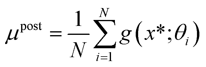 | (5) |
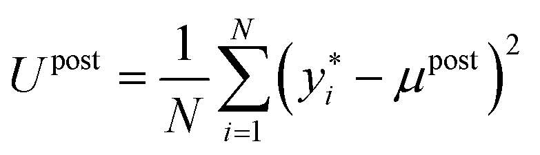 | (6) |
 | (7) |
 is a single sample from the model posterior at new input x*, {θi,σi}Ni=1 are samples from the MCMC chain approximating
  , and N is the total number of MCMC samples. Note that Upost naturally combines both epistemic uncertainty (from the variation in network predictions across different weight samples θi) and aleatoric uncertainty (from the noise terms σi), providing a comprehensive measure of predictive uncertainty.55
The PBNNs are trained in two stages. First, it trains a deterministic neural network, incorporating stochastic weight averaging (SWA)65 at the end of the training trajectory to enhance robustness against noisy training objectives. Second, the probabilistic component is introduced by selecting a subset of layers and using the corresponding pre-trained weights to initialize prior distributions for this subset, while keeping all remaining weights frozen. HMC/NUTS sampling is then applied to derive posterior distributions for the selected subset. Finally, predictions are made by combining both the probabilistic and deterministic components. See Algorithm 1 and Fig. 1 for more details. In certain scenarios, such as autonomous experiments, the entire training process needs to be performed in an end-to-end manner. In these cases, it is crucial to avoid overfitting in the deterministic component, as there will be no human oversight to evaluate its results before transitioning to the probabilistic part. To address this, we incorporate a MAP prior, modeled as a Gaussian penalty, into the loss function during deterministic training. All the PBNNs were implemented via a NeuroBayes package‡ developed by the authors.
 | ||
| Fig. 1 (a) Schematic illustration of Partially Bayesian Neural Network (PBNN) operation. First, we train a deterministic neural network, incorporating stochastic weight averaging to enhance robustness against noisy training objectives. Second, the probabilistic component is introduced by selecting a subset of layers and using the corresponding pre-trained weights to initialize prior distributions for this subset, while keeping all remaining weights frozen. HMC/NUTS sampling is then applied to derive posterior distributions for the selected subset. Finally, predictions are made by combining both the probabilistic and deterministic components. (b) Schematic illustration of flow through a PBNN model alternating probabilistic and deterministic processing stages. | ||
In this work, we have investigated PBNNs of multilayer perceptron (MLP) architecture consisting of five layers: four utilize non-linear activation functions, such as the sigmoid linear unit, while the final (output) layer contains a single neuron without a non-linear activation, as is typical for regression tasks. As there are multiple ways to select probabilistic layers for the PBNNs, we have evaluated the effects of setting different combinations of probabilistic layers as shown in Fig. 2.

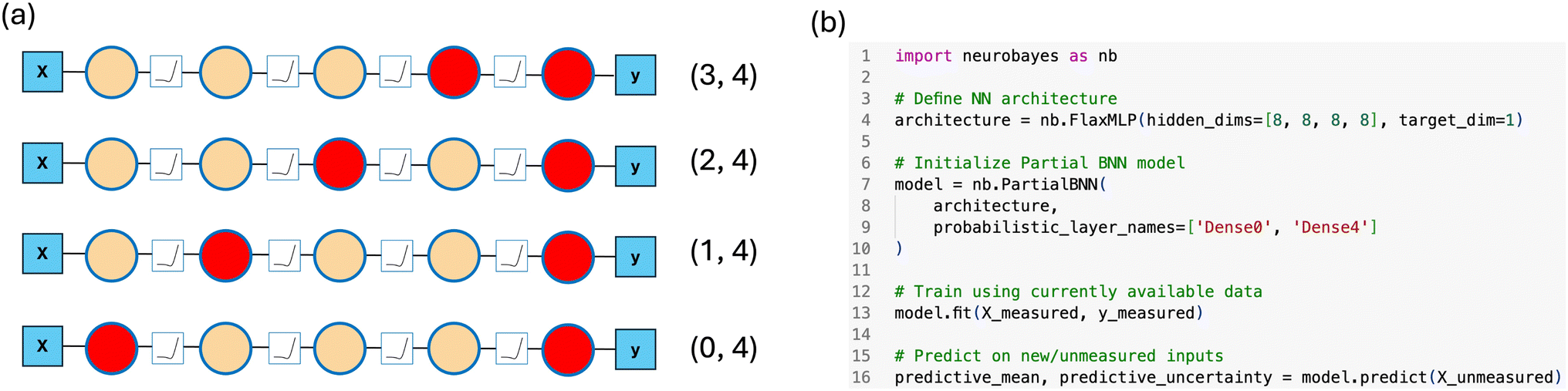 | ||
| Fig. 2 (a) Schematic representation of the partially Bayesian MLP employed in this study. The model consists of five layers: four utilize non-linear activation functions, such as the sigmoid linear unit, while the final (output) layer contains a single neuron without a non-linear activation, as is typical for regression tasks. Circles filled with red denote stochastic layers, while orange filled circles represent deterministic layers. Note that the single output neuron is always made probabilistic, as it often improves training stability. (b) Code snippet illustrating a single train-predict step with PBNN (0, 4). | ||
2.2 Active learning
In AL, the algorithm iteratively identifies points from a pool of unobserved data, within a pre-defined parameter space , that are expected to improve the model's performance in reaching some objective. Starting with an initial, usually small, training dataset
  , an initial PBNN is trained and predictions are made on all
  . The predictions that maximize a suitably selected acquisition function are then selected for measurement via an experiment, simulation, or human labeling. For the sake of benchmarking, we have chosen an acquisition function that simply maximizes the predictive uncertainty, i.e.,
  , and only select a single xnext at each iteration. Note that here we naturally balance exploration between regions of model uncertainty and inherent complexity, as high aleatoric uncertainty often indicates areas requiring additional samples to better estimate noise distributions and capture underlying patterns. For further details regarding the AL algorithm, see Algorithm 2. Usually, this process is repeated until a desired goal is reached or an experimental budget is exhausted; here, we perform 200 exploration steps for all datasets. Lastly, we have selected initial training datasets by randomly sampling subsets of the total datasets containing 5% of the total number of data points. While this procedure results in differently sized initial training datasets, the trends observed are consistent across all datasets and corresponding sizes.
Prediction accuracy was evaluated using the standard root mean square error (RMSE):
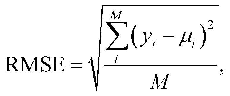 | (8) |
To assess the quality of the predictive uncertainties, we used two metrics, the negative log predictive density (NLPD) and the confidence interval coverage probability, which we refer to as coverage from this point forward. NLPD is given by the following equation:
 | (9) |
NLPD assesses how well a model's predictive distributions align with observed data. A lower NLPD indicates that the model assigns higher probability density to true outcomes while maintaining well-calibrated uncertainty estimates. This metric is valuable for evaluating probabilistic models as it penalizes both overconfident incorrect predictions and underconfident correct ones.
Coverage is given by
 | (10) |
As far as the input features are concerned, we used standard RDKit68 physicochemical descriptors for the molecular datasets. For the steel fatigue dataset, the input features were chemical compositions, upstream processing details, and heat treatment conditions. For the electrical conductivity data, the input features were formed from oxide concentrations, deposition conditions, and processing parameters, such as power settings and gas flow rate. The input features for the Bandgap dataset were derived using the Magpie featurizer, which computes statistical descriptors from elemental properties and composition fractions.69
3 Results and discussion
3.1 Active learning on toy dataset
Before assessing the effectiveness of PBNNs for AL on the materials and molecular datasets, we first analyze their effectiveness on a toy dataset. In particular, we have generated non-stationary data with abrupt changes in frequency and amplitude, a use case where full BNNs consistently outperform GPs.76 We denote PBNN configurations as PBNN (i, 4), where i indicates which hidden layer is probabilistic (counting from 0), and 4 denotes the output layer that is always treated as probabilistic. For example, PBNN (0, 4) has probabilistic first hidden and output layers, while PBNN (3, 4) has probabilistic last hidden and output layers. To ensure fair comparison, all hidden layers have equal width. The output layer consists of a single neuron, so making it probabilistic adds minimal computational overhead while helping with training stability.Fig. 3 shows the evolution of predictions and uncertainty estimates across active learning steps for full BNN (a), PBNN (0,4) (b), and PBNN (3,4) (c). PBNN (0,4) exhibits behavior remarkably similar to full BNN, both in terms of predictive mean and uncertainty estimates (shown as pink shading), while requiring fewer probabilistic layers. In contrast, PBNN (3,4) struggles to provide reliable uncertainty estimates, particularly in regions with strong oscillatory behavior. This is reflected in the performance metrics (d), where PBNN (0,4) closely tracks full BNN's performance while PBNN (3,4) shows consistently higher RMSE and NLPD values, along with coverage probability further from the ideal value of 0.95.
 | ||
| Fig. 3 Active learning results for 1D toy dataset with non-stationary features. Evolution of predictions and uncertainty estimates across active learning steps for (a) full BNN model, (b) model with probabilistic first hidden and output layers, PBNN(0,4), and (c) model with probabilistic last hidden and output layers, PBNN(3,4). Blue lines show predictive mean, pink shading represents uncertainty estimates, and black dashed lines indicate ground truth. Black dots mark noisy observations. Panel (d) compares performance metrics (RMSE, NLPD, and coverage probability) as a function of active learning exploration steps. | ||
3.2 Active learning on molecular datasets
We now investigate the effectiveness of different PBNNs for AL on the standard molecular benchmark datasets. Fig. 4(a) and (b) show RMSE, NLPD, and coverage probability as a function of AL exploration step for ESOL and FreeSolv, respectively. We see that the accuracy and quality of the uncertainties improve with AL for all PBNNs, as demonstrated by (i) decreasing RMSE and NLPD and (ii) coverage approaching 0.95 for all models. Across all metrics for both datasets, making earlier layers probabilistic proves more effective, with PBNN(0,4) approaching the accuracy of a full BNN. Furthermore, PBNN(0,4) exhibits a relatively stable decrease in NLPD and coverage approaching 0.95 throughout the AL process, similar to full BNN. In contrast, configurations where the probabilistic layer is moved away from the first hidden layer, PBNN(1,4), (2,4), and (3,4), show strong oscillatory behavior in NLPD and coverage metrics, suggesting that uncertainty propagation becomes unstable when probabilistic layers are placed in later hidden layers. This shows that, at least within the standard MLP architecture employed here, capturing uncertainty in the first feature transformation layer, combined with a probabilistic output layer, is more effective, both in terms of performance and reliability. In addition, it decreased the overall computational time by nearly a factor of four. Notably, with only a fraction of points explored, AL with PBNN achieves accuracy either comparable to (ESOL) or better than (FreeSolv) that obtained using standard 80![[thin space (1/6-em)]](https://www.rsc.org/images/entities/char_2009.gif) :20 or 90:10 train-test splits with standard deterministic ML models.77
:20 or 90:10 train-test splits with standard deterministic ML models.77
 | ||
| Fig. 4 Comparison of Partially Bayesian Neural Networks (PBNNs) and fully Bayesian neural network (full BNN) on molecular property prediction tasks. (a–c) Aqueous solubility prediction (ESOL database) and (d–f) hydration free energy prediction (FreeSolv database). Each PBNN configuration PBNN (i, 4) has two probabilistic layers: one at position i (counting from 0) and one at the output. Shaded areas represent a standard deviation across five different random seeds. | ||
3.3 Active learning on materials datasets
Next, we follow a similar analysis for the two materials datasets, steel fatigue (NIMS) and conductivity (HTEM), as shown in Fig. 5. We observe overall similar trends to the molecular datasets (decreasing RMSE and NLPD and coverage approaching 0.95), although we see a much stronger difference between the different PBNNs in the uncertainty metrics, with smaller difference in RMSE across different selections of probabilistic layers. We also do not observe the clean monotonic trends that we observed with the molecular datasets for NLPD and coverage on the steel fatigue (NIMS) dataset. This could be due to a variety of factors, but we suspect that this is largely due to differences in the types of input features. While the molecular datasets utilized SMILES-derived descriptors as their input features, the materials datasets contained experimental parameters as their input features, which may not be as predictive of the target properties as the structural SMILES-based descriptors. There could also be a difference in experimental noise between the molecular and materials datasets, as it is well known that values of the materials target properties, fatigue strength and electrical conductivity, are sensitive to experimental variations in their measurement, whereas measurements of hydration free energy and aqueous solubility are relatively standardized. | ||
| Fig. 5 Comparison of Partially Bayesian Neural Networks (PBNNs) and fully Bayesian neural network (full BNN) on materials property prediction tasks. (a–c) Fatigue strength prediction (NIMS database) and (d–f) electrical conductivity prediction (HTEM database). Each PBNN configuration PBNN (i, 4) has two probabilistic layers: one at position i (counting from 0) and one at the output. Shaded areas represent a standard deviation across five different random seeds. | ||
Despite these domain-specific variations, the results across both molecular and materials domains support the emerging general principle that making the first hidden and the output layers probabilistic is more effective than doing so for intermediate or final layers. We would also like to emphasize that we used the same MLP architecture and training parameters (SGD learning rate and iterations for the deterministic component, warmup steps and samples for NUTS in the probabilistic component) across all four datasets. This demonstrates that PBNNs can be relatively robust to hyperparameter selection, a valuable characteristic for practical applications as it minimizes the need for extensive dataset-specific tuning.
3.4 Convergence diagnostics
We next discuss convergence diagnostics for PBNN models during active learning. A popular choice for convergence diagnostics in Bayesian inference is the Gelman–Rubin statistic (‘R-hat’), which provides a measure of convergence for each model parameter.78 However, for Bayesian neural networks, where the parameter space is high-dimensional, examining individual parameter convergence becomes impractical. Instead, we analyzed the distribution of R-hat values across all parameters and found that for the majority of weights (95–99%, depending on dataset), these values lie within acceptable ranges between 1.0 and 1.1.79 While layer-wise or module-wise convergence analysis is also possible for complex architectures, we opted for global parameter statistics due to the relatively simple network structure in this study. See Appendix 1 for more details.†We note that in active learning-based autonomous science tasks, reliable convergence diagnostics play an important role in ensuring the autonomous system performance. The R-hat statistic can therefore serve as an automated quality check, triggering specific actions when convergence issues are detected: for example, if a high proportion (>10%) of parameters display R-hat values outside the acceptable range, the system can employ various convergence improvement heuristics. These include increasing the number of warm-up states, trying different parameter initialization schemes, or adjusting prior distributions. If issues persist after these interventions, the system can flag the experiment for human review, ensuring reliability of the autonomous decision-making process.
3.5 Transfer learning
Transfer learning (TL) is a machine learning method commonly used to improve model performance and/or accelerate training by leveraging knowledge from a related task. TL is particularly valuable when data is limited and difficult to acquire, as is often the case in experimental materials science and chemistry. For deterministic NNs, TL is performed by initializing the network parameters with those of a pre-trained network. Most often the target NN's parameters are still optimized for the task at-hand via backpropagation, which is referred to as fine-tuning.In the context of BNNs, transfer learning can be done through a selection of prior distributions over weights. First, let us revisit how the initial prior distributions are commonly selected. Ideally, the goal of priors in the Bayesian framework is to have a principled way to incorporate domain knowledge. In practice, however, we simply set priors of BNNs to zero-centered normal distributions. This approach provides good regularization and meaningful uncertainty estimates in predictions, but it doesn't incorporate any actual prior domain knowledge. We argue that we can use the weights of a deterministic model trained in a computational (“digital twin”) space to initialize these prior distributions by setting their means to the corresponding pre-trained weights, thereby transferring domain knowledge to a (P)BNN operating in the real world. We can choose to do it for the entire model or only for some parts (layers) of it. We can also specify a “degree of trust” in the theory by selecting appropriate standard deviations for these distributions: wider distributions indicate less confidence in the computational model, while narrower ones encode stronger belief in the underlying theory.
Here, we examine how this simulation-to-experiment transfer learning affects AL with (P)BNNs. The process involves first training a deterministic NN on simulation data, then using its weights to inform the (P)BNN surrogate model that guides active learning on experimental data. A schematic showing this joint TL-AL process is shown in Fig. 6(a). We first study the effectiveness of TL via PBNNs using 1D toy data, where we have generated “theoretical” and “experimental” datasets, emulating phase transitions, with the latter introducing an abrupt change in behavior not captured by the theoretical model (Fig. 6(b)). This is a rather common scenario in scientific modeling where theoretical models reflect the overall trend but fail to capture certain experimental phenomena. Such discrepancies are frequently encountered when theoretical models rely on simplifying assumptions and fail to account for complex physical mechanisms. The middle and bottom panels in Fig. 6(b) compare two approaches to addressing this challenge using full BNNs. Using pre-trained priors, informed by the theoretical model, allows the BNN to maintain good predictions in regions where the theory works well while adapting to experimental evidence where it doesn't. In contrast, standard uninformative priors fail to capture a second phase transition and lead to overly conservative uncertainty estimates.
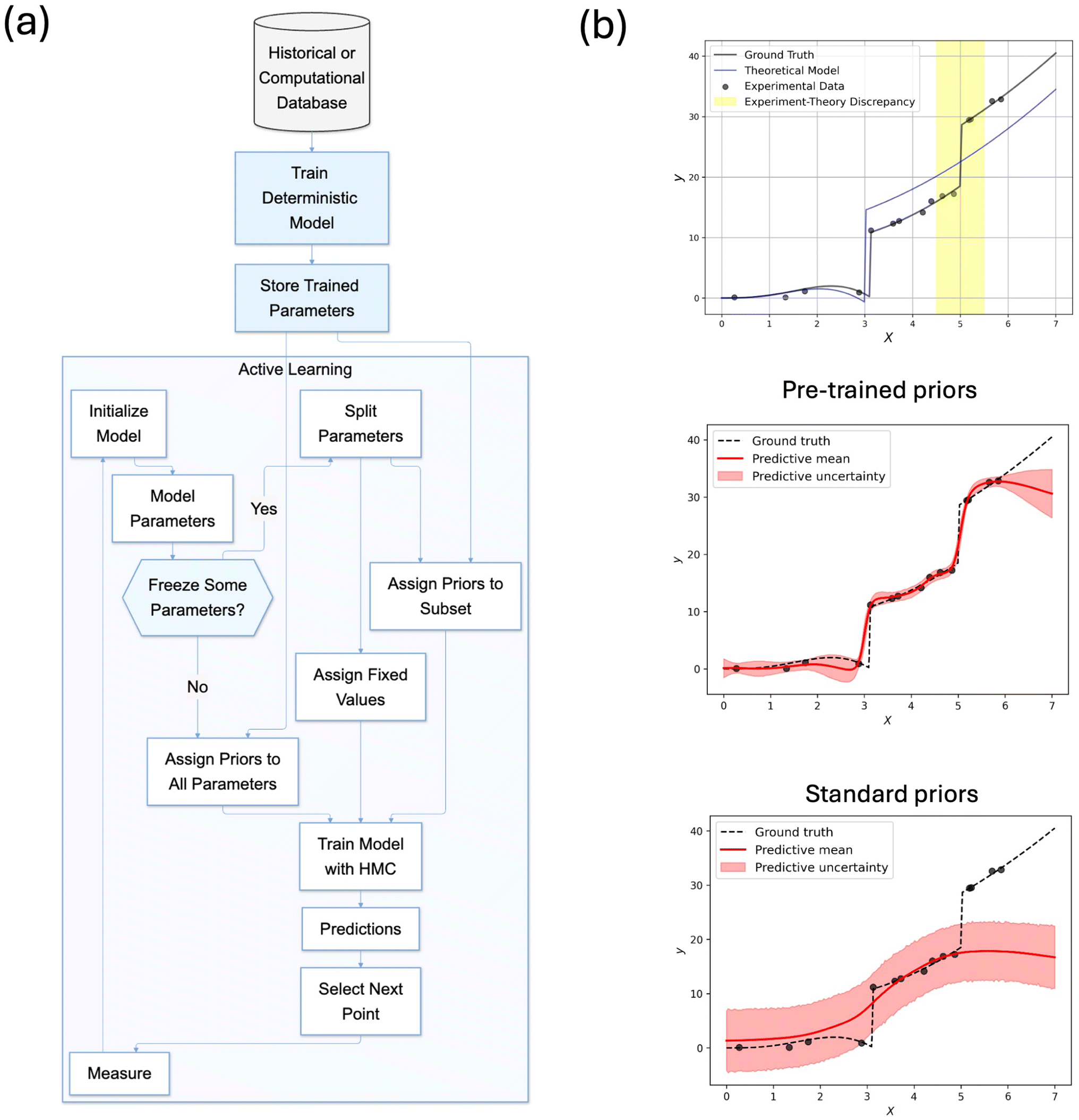 | ||
| Fig. 6 (a) Schematic workflow of transfer learning in active learning: a deterministic model is first trained on historical or computational data, and its parameters are used to initialize and inform priors in the subsequent active learning process. (b) Example predictions comparing BNNs with pre-trained and standard priors. | ||
We now move to the molecular and materials datasets. We start with the Noisy-FreeSolv dataset. Here the deterministic neural network is pre-trained on computational data from molecular dynamics simulations, whereas experimental data is augmented with synthetic noise to create a more challenging test case for our models. For this study, we made the last two hidden layers and the output layer probabilistic, with priors initialized at values of weights from the corresponding pre-trained deterministic neural network. Fig. 7 shows the performance of PBNN with theory-informed priors for different prior widths (τ). While all prior widths demonstrate good performance, wider priors (τ = 0.5, 1.0) outperform narrower priors τ = 0.1 across all metrics. This can be explained by the fact that with small τ values, the prior (informed by the theoretical model) dominates the likelihood in shaping the posterior, failing to account for discrepancy between experiment and theory, whereas with larger values, the likelihood (based on experimental data) starts exerting greater influence. Overall, an ideal value would balance leveraging theoretical knowledge and adapting to experimental observations for a given set of theoretical and experimental data. Comparing pre-trained and standard priors at τ = 1.0, we observe that theory-informed priors lead to substantially better performance across all metrics. The improvement is particularly pronounced in NLPD and coverage, where standard priors show high uncertainty and unstable behavior throughout the active learning process. Finally, we analyze bandgaps of non-metals, where priors are pre-trained on density functional theory (DFT) calculations. Similar to the results observed for Noisy FreeSolv, the results shown in Fig. 8 demonstrate that among different prior widths, there is a clear trade-off: the tight prior (τ = 0.1) shows stable but limited improvement, suggesting it constrains the model too closely to DFT predictions, while wider priors (τ = 0.5 and τ = 1.0) show initial oscillations but ultimately achieve better RMSE through greater adaptation to experimental data. This suggests that one can in principle apply dynamic adjustment: impose a strong belief in the theoretical model initially, and then, as more data becomes available, gradually relax it, allowing the data to speak for itself. Comparing pre-trained and standard priors at τ = 1.0, we observe similar trends to the FreeSolv dataset. The advantage of pre-trained priors is particularly pronounced in the early stages of active learning, where in the first 50 steps they achieve significantly lower RMSE and better calibrated uncertainties compared to standard priors, indicating more efficient use of limited experimental data. While both approaches eventually converge to similar RMSE values, the benefits of pre-trained priors persist in uncertainty quantification throughout the entire process, maintaining substantially better coverage probability.
 | ||
| Fig. 7 Transfer learning with pre-trained PBNNs applied to noisy FreeSolv dataset. (a) RMSE, NLPD, and coverage probability for different prior widths (τ). (b) Comparing the performance of pre-trained priors (τ = 1.0) against standard priors. Shaded areas represent a standard deviation across five different random seeds. | ||
 | ||
| Fig. 8 Transfer learning with pre-trained PBNNs applied to bandgaps dataset. (a–c) RMSE, NLPD, and coverage probability for different prior widths (τ). (d–f) Comparing the performance of pre-trained priors (τ = 1.0) against standard priors. Shaded areas represent a standard deviation across five different random seeds. | ||
4 Conclusion
In this work, we explored the capabilities of partially Bayesian neural networks (PBNNs) in active learning tasks. Within the MLP architectures deployed here, we found that the choice of which layers are made probabilistic significantly impacts performance, with early layers providing better and more stable uncertainty estimates – a finding that held consistently across studied molecular and materials datasets. Notably, PBNNs with probabilistic first layer achieved performance comparable to fully Bayesian networks while requiring substantially fewer computational resources.We further enhanced PBNN performance through transfer learning by initializing priors using theoretical models, which proved particularly beneficial in the early stages of active learning. Our analysis revealed an important trade-off in prior width selection: tight priors ensure stability but may constrain the model too closely to theoretical predictions, while wider priors enable better adaptation to experimental data. Across both studied systems, theory-informed priors led to better calibrated uncertainties and more efficient data utilization.
Overall, this work demonstrates the feasibility of PBNNs for materials science and chemistry, particularly in the context of AL for limited, complex datasets. In the future, we plan to explore the effectiveness of PBNNs across a wider range of architectures, including Graph Neural Networks and Transformers. There may also be interesting connections between our findings about which layers to make probabilistic and emerging research on neural network interpretability, particularly studies that identify specific neurons responsible for distinct behaviors in large language models. Just as certain neurons in LLMs have been found to encode specific linguistic features or semantic concepts, understanding which neurons are most critical for uncertainty quantification could inform more targeted and efficient PBNN architectures.
Data availability
Code and data supporting the paper's findings, together with additional implementation details, are available at https://github.com/ziatdinovmax/NeuroBayes/tree/paper/active_learning_scripts.Conflicts of interest
There are no conflicts to declare.Acknowledgements
This work was supported by the Laboratory Directed Research and Development Program at Pacific Northwest National Laboratory, a multiprogram national laboratory operated by Battelle for the U.S. Department of Energy.References
- D. A. Cohn, Z. Ghahramani and M. I. Jordan, Active learning with statistical models, J. Artif. Intell. Res., 1996, 4(1), 129–145 CrossRef.
- B. Settles, Active Learning Literature Survey, Computer Sciences Technical Report 1648, University of Wisconsin–Madison, 2009, http://axon.cs.byu.edu/%7Emartinez/classes/778/Papers/settles.activelearning.pdf Search PubMed.
- B. Cao, et al., Active learning accelerates the discovery of high strength and high ductility lead-free solder alloys, Mater. Des., 2024, 241, 112921, DOI:10.1016/j.matdes.2024.112921.
- T. Lookman, et al., Active learning in materials science with emphasis on adaptive sampling using uncertainties for targeted design, npj Comput. Mater., 2019, 5, 21, DOI:10.1038/s41524-019-0153-8.
- A. Wang, et al., Benchmarking active learning strategies for materials optimization and discovery, Oxford Open Mater. Sci., 2022, 2(1) DOI:10.1093/oxfmat/itac006.
- P. Xu, et al., Small data machine learning in materials science, npj Comput. Mater., 2023, 9, 42, DOI:10.1038/s41524-023-01000-z.
- B. N. Slautin, et al., Bayesian Conavigation: Dynamic Designing of the Material Digital Twins via Active Learning, ACS Nano, 2024, 18(36), 24898–24908, DOI:10.1021/acsnano.4c05368.
- M. Ziatdinov, et al., Bayesian Active Learning for Scanning Probe Microscopy: From Gaussian Processes to Hypothesis Learning, ACS Nano, 2022, 16(9), 13492–13512, DOI:10.1021/acsnano.2c05303.
- R. Arróyave, Phase Stability Through Machine Learning, J. Phase Equilib. Diffus., 2022, 43(6), 606–628, DOI:10.1007/s11669-022-01009-9.
- I. Peivaste, E. Jossou and A. A. Tiamiyu, Data-driven analysis and prediction of stable phases for high-entropy alloy design, Sci. Rep., 2023, 13(1), 22556, DOI:10.1038/s41598-023-50044-0.
- S. Liu, et al., A comparative study of predicting high entropy alloy phase fractions with traditional machine learning and deep neural networks, npj Comput. Mater., 2024, 10, 172, DOI:10.1038/s41524-024-01335-1.
- H. Xiang, et al., Exploring high thermal conductivity polymers via interpretable machine learning with physical descriptors, npj Comput. Mater., 2023, 9, 191, DOI:10.1038/s41524-023-01154-w.
- Y. Luo, et al., Predicting lattice thermal conductivity via machine learning: a mini review, npj Comput. Mater., 2023, 9, 4, DOI:10.1038/s41524-023-00964-2.
- N. K. Barua, et al., Interpretable Machine Learning Model on Thermal Conductivity Using Publicly Available Datasets and Our Internal Lab Dataset, Chem. Mater., 2024, 36(14), 7089–7100, DOI:10.1021/acs.chemmater.4c01696.
- J. Carrete, et al., Finding Unprecedentedly Low-Thermal-Conductivity Half-Heusler Semiconductors via High-Throughput Materials Modeling, Phys. Rev. X, 2014, 4(1), 011019, DOI:10.1103/PhysRevX.4.011019.
- C. Liu and H. Su, Prediction of glass transition temperature of oxide glasses based on interpretable machine learning and sparse data sets, Mater. Today Commun., 2024, 40, 109691, DOI:10.1016/j.mtcomm.2024.109691.
- J. Zhang, et al., Data-driven machine learning prediction of glass transition temperature and the glass-forming ability of metallic glasses, Nanoscale, 2023, 15(45), 18511–18522, 10.1039/D3NR04380K.
- G. Armeli, J. H. Peters and T. Koop, Machine-Learning-Based Prediction of the Glass Transition Temperature of Organic Compounds Using Experimental Data, ACS Omega, 2023, 8(13), 12298–12309, DOI:10.1021/acsomega.2c08146.
- T. Galeazzo and M. Shiraiwa, Predicting glass transition temperature and melting point of organic compounds via machine learning and molecular embeddings, Environ. Sci.: Atmos., 2022, 2(3), 362–374, 10.1039/d1ea00090j.
- M. J. Uddin and J. Fan, Interpretable Machine Learning Framework to Predict the Glass Transition Temperature of Polymers, Polymers, 2024, 16(8) DOI:10.3390/polym16081049.
- Y. Hu, et al., Accurate prediction of dielectric properties and bandgaps in materials with a machine learning approach, Appl. Phys. Lett., 2024, 125(15), 152905, DOI:10.1063/5.0223890.
- S. S. Dong, M. Govoni and G. Galli, Machine learning dielectric screening for the simulation of excited state properties of molecules and materials, Chem. Sci., 2021, 12(13), 4970–4980, 10.1039/d1sc00503k.
- M. Grumet, et al., Delta Machine Learning for Predicting Dielectric Properties and Raman Spectra, J. Phys. Chem. C, 2024, 128(15), 6464–6470, DOI:10.1021/acs.jpcc.4c00886.
- Y. Shimano, A. Kutana and R. Asahi, Machine learning and atomistic origin of high dielectric permittivity in oxides, Sci. Rep., 2023, 13(1), 22236, DOI:10.1038/s41598-023-49603-2.
- D. Morgan and R. Jacobs, Opportunities and Challenges for Machine Learning in Materials Science, Annu. Rev. Mater. Res., 2020, 50(1), 71–103, DOI:10.1146/annurev-matsci-070218-010015.
- S. S. Chong, et al., Advances of machine learning in materials science: Ideas and techniques, Front. Phys., 2023, 19, 13501, DOI:10.1007/s11467-023-1325-z.
- X. Zhong, et al., Explainable machine learning in materials science, npj Comput. Mater., 2022, 8, 204, DOI:10.1038/s41524-022-00884-7.
- J. Schmidt, et al., Recent advances and applications of machine learning in solid-state materials science, npj Comput. Mater., 2019, 5, 83, DOI:10.1038/s41524-019-0221-0.
- S. Wager, T. Hastie and B. Efron, Confidence intervals for random forests: the jackknife and the infinitesimal jackknife, J. Mach. Learn. Res., 2014, 15(1), 1625–1651 Search PubMed.
- C. Guo et al., On calibration of modern neural networks, in Proceedings of the 34th International Conference on Machine Learning - Volume 70. ICML'17, JMLR.org, Sydney, NSW, Australia, 2017, pp. 1321–1330 Search PubMed.
- B. He, et al., FFMDFPA: A FAIRification Framework for Materials Data with No-Code Flexible Semi-Structured Parser and Application Programming Interfaces, J. Chem. Inf. Model., 2023, 63(16), 4986–4994, DOI:10.1021/acs.jcim.3c00836.
- L. Himanen, et al., Data-Driven Materials Science: Status, Challenges, and Perspectives, Adv. Sci., 2019, 6(21), 1900808, DOI:10.1002/advs.201900808.
- D. Jha, et al., Enhancing materials property prediction by leveraging computational and experimental data using deep transfer learning, Nat. Commun., 2019, 10(1), 5316, DOI:10.1038/s41467-019-13297-w.
- C. E. Rasmussen and C. K. I. Williams, Gaussian Processes for Machine Learning, The MIT Press, 2005 Search PubMed.
- J. Snoek, H. Larochelle and R. P. Adams, Practical Bayesian Optimization of Machine Learning Algorithms, in Advances in Neural Information Processing Systems, ed. F. Pereira, et al., Curran Associates, Inc., 2012, vol. 25, https://proceedings.neurips.cc/paper_files/paper/2012/file/05311655a15b75fab86956663e1819cd-Paper.pdf Search PubMed.
- R. Gramacy. Surrogates: Gaussian Process Modeling, Design, and Optimization for the Applied Sciences, 2020 Search PubMed.
- V. L. Deringer, et al., Gaussian process regression for materials and molecules, Chem. Rev., 2021, 121(16), 10073–10141 CrossRef CAS PubMed.
- R. Calandra, et al., Manifold Gaussian Processes for regression, in 2016 International Joint Conference on Neural Networks (IJCNN), 2016, pp. 3338–3345 Search PubMed.
- A. G. Wilson, et al., Deep Kernel Learning, in Proceedings of the 19th International Conference on Artificial Intelligence and Statistics, ed. A. Gretton and C. C. Robert, PMLR, Cadiz, Spain, 2016, vol. 51. Proceedings of Machine Learning Research, pp. 370–378, https://proceedings.mlr.press/v51/wilson16.html Search PubMed.
- A. G. Wilson, et al., Stochastic variational deep kernel learning, in Proceedings of the 30th International Conference on Neural Information Processing Systems. NIPS'16: Curran Associates Inc., Barcelona, Spain, 2016, pp. 2594–2602 Search PubMed.
- S. Singh and J. M. Hernandez-Lobato, Deep Kernel learning for reaction outcome prediction and optimization, Commun. Chem., 2024, 7(1), 136, DOI:10.1038/s42004-024-01219-x.
- K. Duhrkop, Deep kernel learning improves molecular fingerprint prediction from tandem mass spectra, Bioinformatics, 2022, 38(Suppl 1), i342–i349, DOI:10.1093/bioinformatics/btac260.
- M. Valleti, et al., Deep kernel methods learn better: from cards to process optimization, Mach. Learn.: Sci. Technol., 2024, 5, 015012, DOI:10.1088/2632-2153/ad1a4f.
- S. W. Ober, C. E. Rasmussen, and M. van der Wilk. The promises and pitfalls of deep kernel learning, in Proceedings of the Thirty-Seventh Conference on Uncertainty in Artificial Intelligence. ed. C. de Campos and M. H. Maathuis, 2021, vol. 161. Proceedings of Machine Learning Research. PMLR, pp. 1206–1216, https://proceedings.mlr.press/v161/ober21a.html Search PubMed.
- D. M. Titterington, Bayesian Methods for Neural Networks and Related Models, Stat. Sci., 2004, 19(1), 128–139, DOI:10.1214/088342304000000099.
- J. Lampinen and A. Vehtari, Bayesian approach for neural networks—review and case studies, Neural Netw., 2001, 14(3), 257–274 CrossRef CAS PubMed.
- A. Nguyen, J. Yosinski, and J. Clune, Deep neural networks are easily fooled: High confidence predictions for unrecognizable images, Conference Paper, 2015, DOI:10.1109/CVPR.2015.7298640.
- D. Hendrycks and K. Gimpel, A Baseline for Detecting Misclassified and Out-of-Distribution Examples in Neural Networks, Conference Paper, 2017 Search PubMed.
- B. Lakshminarayanan, A. Pritzel and C. Blundell, Simple and Scalable Predictive Uncertainty Estimation using Deep Ensembles, Conference Paper, 2017 Search PubMed.
- W. K. Hastings, Monte Carlo Sampling Methods Using Markov Chains and Their Applications, Biometrika, 1970, 57(1), 97–109 CrossRef.
- D. M. Blei, A. Kucukelbir and J. D. McAuliffe, Variational Inference: A Review for Statisticians, J. Am. Stat. Assoc., 2017, 112(518), 859–877, DOI:10.1080/01621459.2017.1285773.
- M. Betancourt, A Conceptual Introduction to Hamiltonian Monte Carlo, arXiv, 2018, preprint, arXiv:1701.02434[stat.ME], DOI:10.48550/arXiv.1701.02434.
- Y. Yao, et al., Yes, but Did It Work?: Evaluating Variational Inference, in Proceedings of the 35th International Conference on Machine Learning, ed. J. Dy and A. Krause, 2018, vol. 80. Proceedings of Machine Learning Research. PMLR, pp. 5581–5590, https://proceedings.mlr.press/v80/yao18a.html Search PubMed.
- M. D. Homan and A. Gelman, The No-U-turn sampler: adaptively setting path lengths in Hamiltonian Monte Carlo, J. Mach. Learn. Res., 2014, 15(1), 1593–1623 Search PubMed.
- A. Kendall and Y. Gal, What uncertainties do we need in Bayesian deep learning for computer vision?, in Proceedings of the 31st International Conference on Neural Information Processing Systems. NIPS'17, Curran Associates Inc., Long Beach, California, USA, 2017, pp. 5580–5590 Search PubMed.
- B. Charles, et al., Weight Uncertainty in Neural Network, in Proceedings of the 32nd International Conference on Machine Learning, ed. F. Bach and D. Blei, PMLR, Lille, France, 2015, vol. 37. Proceedings of Machine Learning Research, pp. 1613–1622, https://proceedings.mlr.press/v37/blundell15.html Search PubMed.
- E. Daxberger, et al., Laplace Redux - Effortless Bayesian Deep Learning, in Advances in Neural Information Processing Systems, ed. M. Ranzato, et al., Curran Associates, Inc., 2021, vol. 34, pp. 20089–20103, https://proceedings.neurips.cc/paper_files/paper/2021/file/a7c9585703d275249f30a088cebba0ad-Paper.pdf Search PubMed.
- R. M. Neal, Bayesian Learning for Neural Networks, Lecture Notes in Statistics, Springer, New York, 2012, https://books.google.com/books?id=LHHrBwAAQBAJ Search PubMed.
- M. Welling and Y. Whye Teh, Bayesian learning via stochastic gradient langevin dynamics, in Proceedings of the 28th International Conference on International Conference on Machine Learning. ICML'11, Omnipress, Bellevue, Washington, USA, 2011, pp. 681–688 Search PubMed.
- A. Y. K. Foong, et al., On the expressiveness of approximate inference in Bayesian neural networks, in Proceedings of the 34th International Conference on Neural Information Processing Systems. NIPS '20, Curran Associates Inc., Vancouver, BC, Canada, 2020 Search PubMed.
- A. K. D. M. Blei and J. D. McAuliffe, Variational Inference: A Review for Statisticians, J. Am. Stat. Assoc., 2017, 112(518), 859–877, DOI:10.1080/01621459.2017.1285773.
- S. Rossi, P. Michiardi and M. Filippone, Good Initializations of Variational Bayes for Deep Models, in Proceedings of the 36th International Conference on Machine Learning, ed. K. Chaudhuri and R. Salakhutdinov, 2019. vol. 97. Proceedings of Machine Learning Research. PMLR, pp. 5487–5497, https://proceedings.mlr.press/v97/rossi19a.html Search PubMed.
- M. Sharma, et al., Do Bayesian Neural Networks Need To Be Fully Stochastic?, arXiv, 2023, preprint, arXiv:2211.06291[cs.LG], DOI:10.48550/arXiv.2211.06291.
- J. Harrison, J. Willes and J. Snoek, Variational Bayesian Last Layers, arXiv, 2024, preprint, arXiv:2404.11599[cs.LG], DOI:10.48550/arXiv.2404.11599.
- P. Izmailov, et al., Averaging Weights Leads to Wider Optima and Better Generalization, arXiv, 2019, preprint, arXiv:1803.05407[cs.LG], DOI:10.48550/arXiv.1803.05407.
- B. Kompa, J. Snoek and A. L. Beam, Empirical Frequentist Coverage of Deep Learning Uncertainty Quantification Procedures, Entropy, 2021, 23(12), 1608, DOI:10.3390/e23121608.
- L. Sluijterman, E. Cator and T. Heskes, How to evaluate uncertainty estimates in machine learning for regression?, Neural Netw., 2024, 173, 106203, DOI:10.1016/j.neunet.2024.106203.
- RDKit Contributors, RDKit: Open-source cheminformatics, https://www.rdkit.org Search PubMed.
- L. Ward, et al., A general-purpose machine learning framework for predicting properties of inorganic materials, npj Comput. Mater., 2016, 2(1), 1–7 CrossRef.
- D. L. Mobley and J. P. Guthrie, FreeSolv: a database of experimental and calculated hydration free energies, with input files, J. Comput.-Aided Mol. Des., 2014, 28(7), 711–720, DOI:10.1007/s10822-014-9747-x.
- J. S. Delaney, ESOL: Estimating Aqueous Solubility Directly from Molecular Structure, J. Chem. Inf. Comput. Sci., 2004, 44(3), 1000–1005, DOI:10.1021/ci034243x.
- A. Agrawal, et al., Exploration of data science techniques to predict fatigue strength of steel from composition and processing parameters, Integr. Mater. Manuf. Innov., 2014, 3, 90–108, DOI:10.1186/2193-9772-3-8.
- A. Zakutayev, et al., An open experimental database for exploring inorganic materials, Sci. Data, 2018, 5, 180053, DOI:10.1038/sdata.2018.53.
- A. Jain, et al., Commentary: The Materials Project: A materials genome approach to accelerating materials innovation, APL Mater., 2013, 1(1), 011002, DOI:10.1063/1.4812323.
- Ya Zhuo, A. M. Tehrani and J. Brgoch, Predicting the Band Gaps of Inorganic Solids by Machine Learning, J. Phys. Chem. Lett., 2018, 9(7), 1668–1673, DOI:10.1021/acs.jpclett.8b00124.
- M. Ziatdinov, Active Learning with Fully Bayesian Neural Networks for Discontinuous and Nonstationary Data, arXiv, 2024, preprint, arXiv:2405.09817[cs.LG], DOI:10.48550/arXiv.2405.09817.
- Z. Wu, et al., MoleculeNet: A Benchmark for Molecular Machine Learning, arXiv, 2018, preprint, arXiv:1703.00564[cs.LG], DOI:10.48550/arXiv.1703.00564.
- A. Gelman and D. B. Rubin, Inference from Iterative Simulation Using Multiple Sequences, Stat. Sci., 1992, 7(4), 457–472, DOI:10.1214/ss/1177011136.
- S. P. Brooks and A. Gelman, General Methods for Monitoring Convergence of Iterative Simulations, J. Comput. Graph. Stat., 1998, 7(4), 434–455, DOI:10.1080/10618600.1998.10474787.
Footnotes |
| † Electronic supplementary information (ESI) available. See DOI:https://doi.org/10.1039/d5dd00027k |
| ‡ https://github.com/ziatdinovmax/NeuroBayes |
| This journal is © The Royal Society of Chemistry 2025 |