Enhancing predictive models for solubility in multicomponent solvent systems using semi-supervised graph neural networks

Abstract

Solubility plays a critical role in guiding molecular design, reaction optimization, and product formulation across diverse chemical applications. Despite its importance, current approaches for measuring solubility face significant challenges, including time- and resource-intensive experiments and limited applicability to novel compounds. Computational prediction strategies, ranging from theoretical models to machine learning (ML) based methods, offer promising pathways to address these challenges. However, such methodologies need further improvement to achieve accurate predictions of solubilities in multicomponent solvent systems, as expanding the modeling approaches to multicomponent mixtures enables broader practical applications in chemistry. This study focuses on modeling solubility in multicomponent solvent systems, where data scarcity and model generalizability remain key hurdles. We curated a comprehensive experimental solubility dataset (MixSolDB) and examined two graph neural network (GNN) architectures – concatenation and subgraph – for improved predictive performance. By further integrating computationally derived COSMO-RS data via a teacher–student semi-supervised distillation (SSD) framework, we significantly expanded the chemical space and corrected previously high error margins. These results illustrate the feasibility of unifying experimental and computational data in a robust, flexible GNN-SSD pipeline, enabling greater coverage, improved accuracy, and enhanced applicability of solubility models for complex multicomponent solvent systems.

---

Introduction

Solubility, defined as the equilibrium concentration of a solute at saturation, is a fundamental property that influences a wide range of chemical applications. The role of solubility is pivotal, as it governs the rate of diffusion, the formation of molecular complexes, the kinetics of reactions, and the final material properties of substances, thereby influencing every stage of chemical manipulation and analysis. Without proper attention to solubility, the design and optimization of chemical processes may not fully meet their intended goals of obtaining target chemicals. In the pharmaceutical industry, for example, water and organic solvent solubility guide drug candidate screening, synthetic strategies, and bioavailability during the entire development process.^1–10 Moreover, understanding kinetic solvent effects is crucial for choosing appropriate solvents to control the solubility of reacting species, influencing both the reaction pathway and the product selectivity.^11–22 This concept extends to research areas such as sustainable chemistry and renewable energy, where controlling water solubility can help manage contaminants from crude oil refining, and optimization of solvent can enhance catalytic activity in biomass upgrading to biofuels and renewable polymers.^23–26

Although one can experimentally measure solubilities to design fit-for-purpose solvent systems, experiments are often time-consuming, resource-intensive, and pose challenges for compounds that have yet to be synthesized. Furthermore, there is no universally reliable method for solubility measurements because of varying experimental conditions, such as agitation and solvent composition, which can influence the measured values.²⁷ As a result, computational solubility prediction has emerged as an attractive alternative, with two main approaches gaining prominence: theoretical and data-driven methods. Theoretical approaches, such as those based on quantum mechanics (QM) and molecular dynamics (MD), approximate solvation energies by parameterizing or sampling solute–solvent interactions, either implicitly or explicitly. Although these methods can give accurate results for certain systems, they frequently require substantial time and computational resources, particularly when modeling explicit solvent environments.^28,29 Moreover, the resulting solubility predictions, in some cases with increasing complexity, deviate systematically from experimental data in QM-based models like COnductor-like Screening MOdel for Real Solvents (COSMO-RS), Solvation Model based on Density (SMD), and other implicit solvation frameworks.^30–37

In contrast to theoretical approaches, data-driven methods, particularly those employing machine learning (ML), can rapidly predict solubility once models are trained.^38–46 Recent advances include the use of graph neural networks (GNNs),^47–49 recurrent neural networks,⁴⁵ and transformer-based models originally developed for natural language processing.⁵⁰ These ML techniques have been extended to predict solubility at various temperatures,⁵¹ guiding the design of molecules with optimal solubility in a variety of solvent systems.^49,52 However, achievement of high accuracy with ML models depends heavily on the size, diversity, and quality of training data. Many models often struggle to generalize to novel compounds not represented in the training set. In particular, GNN-based architectures often require hundreds of thousands of datapoints to achieve reliable predictions.^48,53

These challenges become even more distinct in multicomponent solvent systems. Recently, there has been much interest in using mixtures of multiple solvents to precisely tune solvation behavior for a variety of industrial processes; as opposed to single-solvent systems, the use of multiple solvents allows chemists fine-grained control over solvation-based processes. For instance, controlling solubility supports the extraction of aromatic components from oils with impurities to improve fuel quality and efficiency.^54–56 Similarly, understanding solubility behavior in multicomponent solvent systems is key to optimizing product extraction, as demonstrated by using hexane–ethyl acetate–methanol–water (HEMWat) solvent system to separate lignin-derived monomers.²⁶ Moreover, the selection of appropriate cosolvents can also enhance the solubility of water-insoluble drugs, thereby expanding their therapeutic potential.^57,58 There are several studies using ML approaches to broaden chemical space coverage for multicomponent solvent systems.^59,60 However, the requirement of understanding the interactions between multiple solvents hampers the applicability of conventional ML models, as each solvent potentially influences solute behavior through distinct molecular interactions. As a result, building reliable ML models for multicomponent systems not only demands more qualified data but also sophisticated modeling approaches considering the complex relationship between solute and solvents.

Our group has previously developed GNN models for the prediction of solubility in single solvent systems.⁴⁹ Based on our previous work, this report is motivated by the need to address the challenge of accurately modeling solubility in multicomponent solvent systems. After curating a dataset of experimental solubilities in multicomponent solvents from the literature containing up to three solvents, we developed and analyzed two modeling architectures: ‘concatenation’ and ‘subgraph’. By identifying the most promising architecture and augmenting a limited experimental dataset with computationally generated data, we expanded the chemical space covered and improved prediction reliability through a semi-supervised distillation (SSD) framework.

Methods

Solvation free energy database

Curation of experimental solvation free energy. As part of this work, we developed an extensive new database (MixSolDB) for small molecule solubility, containing solvation free energy values (ΔG_solv.) in single, binary, and ternary solvent systems. We meticulously curated experimental measurements from previously published literature, with each entry accompanied by an attributing reference. In addition to our solubility data curations, we also integrated data from previously published database⁵⁹ to create MixSolDB. The complete MixSolDB is publicly available for distribution through our GitHub page,⁶¹ providing easy access to researchers.

Experimental solubility datasets are labeled by either molar solubility (log S) or solvation free energy (ΔG_solv.). Our focus is on ΔG_solv. because it represents the thermodynamic stability of a solute in a solvent, being governed solely by solute–solvent interaction, whereas log S directly quantifies the solute concentration. To maintain the consistency across the datapoints in MixSolDB, we used the following equation for unit conversion from molar solubility (S) to solvation free energy (ΔG_solv.)⁶²

where R is the gas constant, T is temperature, S is the solubility of the solute in molarity unit, M° is the standard state molarity (1 mol L⁻¹), P_vap is the vapor pressure of the solute in equilibrium with its pure liquid, and P° is the pressure of an ideal gas at 1 mol L⁻¹ and 298 K (24.45 atm). For this unit conversion, the vapor pressure of each solute molecule was needed, so we developed a separate prediction model for vapor pressure prediction, and details can be found in subsection ‘Assembling a comprehensive solubility dataset (MixSolDB)’ of Results and discussion section. Notably, the thermodynamic procedure of converting log S data to the Gibbs free energy of solvation ΔG_solv. relies solely on reputable experimental references and does not involve predictions from our solubility model. This ensures the database remains experimentally grounded, without data leakage from predictive modeling steps.

Computational details for solvation free energy calculation. In this work, we also calculated solvation free energy values (ΔG_solv.) for novel solute–solvent combinations for which no experimental measurements are available. This calculated database was used for augmenting data used for training our models. Solvation free energy was calculated based on quantum mechanical COSMO-RS theory,^35,63,64 utilizing COSMOTherm program.⁶⁵ For practical use, polarization charges of each solute and solvent molecule in a continuum were calculated at the BVP86/TZVP/DGA1 theoretical level.

ML model details. All ML models developed were trained in Python 3.8.13 using the following packages: TensorFlow 2.9.1, Keras 2.9.0, RDKit 2022.3.5, and Neural Fingerprint (NFP) 0.3.0. Model metrics for all models were calculated via Scikit-Learn functions where available or using NumPy when not. The GNN used mean absolute error (MAE) as the loss function and Adam as the optimizer, with a batch size of 1024 with 1000 epochs. The ReduceLROnPlateau TensorFlow callback was used to determine the model learning rate, with an initial learning rate of 1 × 10⁻⁴, a factor of 0.5 with patience of 5 epochs, and a minimum learning rate of 1 × 10⁻⁶.

Unless stated otherwise, all graph neural network (GNN) models were trained using an 80/10/10 train/validation/test split. In the standard GNN architecture used, each model has two separate GNN blocks: an intramolecular GNN and an intermolecular GNN. The intramolecular GNN was the same for all models trained, while the intermolecular GNN was either a “subgraph” or “concatenation” based architecture. For a given datapoint, there is one intramolecular GNN for each chemical species (solute/solvent 1/…/solvent N) which feeds their output into an intermolecular GNN. The output of the intermolecular GNN is the predicted solvation free energy values (ΔG_solv.) for the respective input (solute identity, solvent system identity and stoichiometry, and temperature).

Results and discussion

Assembling a comprehensive solubility dataset (MixSolDB)

We assembled a comprehensive dataset of experimental solubilities totaling 56 789 entries, which included 11 609 measured solvation free energy values and 45 180 values expressed as the logarithm of molar solubility (Fig. 1A). To accurately convert between these units, we required reliable estimates of vapor pressure for each solute. Since the vapor pressure is commonly estimated using the Antoine equation, we developed a dedicated prediction model to determine its three compound-specific Antoine parameters, A, B, and C. The Antoine equation is an empirical formula that relates vapor pressure to temperature:where P is the vapor pressure (in atm), T is the temperature (in °C), and A, B, and C are substance-dependent parameters.

Fig. 1 (A) Composition of datapoints in MixSolDB: data units and solvent system categories. (B) Distribution of solvation free energy curated in MixSolDB.

Fig. 2 provides a schematic overview of our vapor pressure prediction model. The model processes molecular structures by first embedding atom and bond features into 128-dimensional vectors. Atom-level features include chemical symbol, hydrogen count, aromaticity, and ring state, while bond-level features encode bond type, connectivity (start and end atom), ring state, and global features that incorporate hydrogen bonding capabilities. These embeddings are then passed through a series of five message passing layers in the GNN model used by our group's previous work on cetane number prediction for single compounds,⁶⁶ to refine the internal molecular representation iteratively. The resulting latent vector is finally fed into a dense output layer that predicts the three Antoine parameters. This end-to-end learned representation enables the model to relate molecular structure to its vapor pressure behavior effectively.

Fig. 2 Model structure for vapor pressure prediction.

To develop and validate this approach, we employed the published database,⁶⁷ curating Antoine parameters of organic liquids from the Yaws Handbook. The dataset encompasses a chemical space of 23 346 compounds, predominantly composed of carbon (C) and hydrogen (H), with up to 100 carbon and 202 hydrogen atoms per molecule. A range of heteroatoms are also present, most notably oxygen (O), halogens (Cl, F, Br, I), sulfur (S), and nitrogen (N), with oxygen found in over 9000 compounds and halogens appearing in thousands more. Less common elements such as silicon (Si), phosphorus (P), selenium (Se), arsenic (As), and various metals (e.g., Hg, In, Ni, Zn) appear in a smaller subset of molecules. The values in the database span a broad range: A values fall between 1.03 and 127.89 (mean 4.52), B ranges from 136.85 to 500 000 (mean 2100.42), and C ranges from −83.1 to 3943.49 (mean 182.35). After tuning hyperparameters and conducting 5-fold cross-validation, our final configuration – featuring a learning rate of 1.0 × 10⁻³, five graph neural network layers, and 64 hidden nodes – yielded mean test set mean absolute errors (MAEs) of 1.24, 67.8, and 7.83 for A, B, and C, respectively, with corresponding standard deviations of 0.77, 11.72, and 0.8. Although the MAEs for B, and C appear larger, it should be noted that B is divided by (C + T) in the Antoine equation, effectively reducing the impact of a larger absolute error. Moreover, the MAE of A is quite small when compared to its overall range, indicating our model's strong performance. Overall, these errors remain marginal and illustrate the capability of our method to provide accurate vapor pressure estimates. By integrating these Antoine parameters into our workflow, we enhanced the reliability of unit conversions and, consequently, improved the overall consistency of our solubility dataset, MixSolDB. Although our vapor pressure prediction model achieves robust accuracy in predicting Antoine parameters for the dataset curated from the Yaws Handbook, we recognize that the chemical space of the curated datapoints may not capture the full diversity of vapor pressure behaviors. Consequently, systematic uncertainties stemming from the limited scope of the training data could propagate into subsequent solvation free energy calculations, prompting caution when applying this model beyond its current domain.

The resulting MixSolDB dataset spans a broad choice of molecules, comprising 11 796 unique solutes and 1445 unique solvents distributed across 56 789 total datapoints (Fig. 1A and B). This collection includes 25 909 single solvent, 29 158 binary solvent, and 1722 ternary solvent datapoints, ensuring coverage of a wide range of compositional complexities. The solvation free energy values range from −33.74 to 24.58 kcal mol⁻¹, and the largest bins in each color represent 12% of single solvent, 12% of binary solvent, and 51% of ternary solvents. Additionally, the dataset encompasses temperatures from 252.55 K up to 368.15 K. The distribution of functional groups of solute molecules is reported in Table S1† to identify the most common and less frequent derivatives.

Despite its considerable diversity, MixSolDB still covers only a small fraction of the full combinatorial chemical space. Although it includes 11 778 unique solutes for single solvent systems, the number of solutes present in binary and ternary solvent combinations is much smaller – 174 and 3, respectively – highlighting the limited entries in more complex mixtures. While the overall number of unique solutes is large, it does not translate into proportional increases in solute–solvent pair or multicomponent solvent combinations. As a result, this dataset, despite its size, represents only a narrow slice of the vast chemical complexity of solutions. Moving forward, it is imperative to expand MixSolDB's diversity by systematically increasing both solute and solvent types, particularly in multicomponent solvent systems. We discuss about how we expanded the diversity of MixSolDB in the following sections.

Expanding solubility modeling with subgraph GNN strategies: insights into binary and ternary mixtures

To accurately model solubility, it is essential to consider both the intramolecular interactions inherent to the chemical species of interest and the intermolecular interactions occurring between different components in solution. By intermolecular, we refer to the interactions between multiple molecules (e.g., solute–solute, solute–solvent, and solvent–solvent interactions). Previous work has demonstrated that a directed message passing neural network (D-MPNN) can effectively capture intramolecular interactions, making it well suited for predicting the solubility of a solute within a single solvent system.^52–54

A widely used approach to extending these methods to the multicomponent solvent system is the so-called “concatenation GNN” (Fig. 3A). In this method, separate representations of the solute and solvents are concatenated to create a combined solute–solvent vector, which is then processed through sequential neural network layers. Although this strategy has proven effective,^68–70 it becomes increasingly vulnerable to permutation equivariance as the number of components increases, making it less robust for complex mixtures. Moreover, it remains unclear whether solvent representations should be pre-pooled before concatenation or if it is more beneficial to integrate solute and solvent interactions in a stepwise, iterative fashion. To address these challenges, we have developed a novel scheme for representing multicomponent solvent systems termed here as the “subgraph GNN” approach (Fig. 3B). While subgraph neural networks have been explored for a variety of prediction tasks,^71,72 this work presents the first in-depth study using subgraph GNNs to predict multicomponent solubility. Our approach employs a fully connected subgraph to ensure thorough consideration of mixing effects among solutes and solvents, although this constraint is not fundamental and can be relaxed to model other systems or to incorporate additional inductive biases. In particular, the subgraph GNN framework can embed chemically relevant information into edge states, including molecular size via molar mass, molecular shape via the Balaban J index, and hydrogen bonding information via the number of hydrogen bond acceptors/donors (Fig. 4). By incorporating these properties directly into the edge connections between components, the subgraph GNN offers a flexible and chemically informed model.

Fig. 3 Schematic diagram of the intramolecular component of our solubility prediction architecture alongside the two methods used for modeling intermolecular interactions.

Fig. 4 Detailed model architectures for the concatenation model and subgraph model.

Under conditions where every solute–solvent pair is fully connected, the concatenation and subgraph GNN strategies share some conceptual similarities in that both require the pooling of solute and solvent features followed by neural network refinements with dense layer updates. Crucially, however, the subgraph approach re-adds the dense embeddings of the original solute and solvent nodes through skip connections that follow each node and edge update step (Fig. 4, right). This design reduces the amount of solute and solvent information lost or diluted during the subsequent dense updates while preserving information on both solute–solvent interactions and solute–solute/solvent–solvent interactions. Moreover, the subgraph GNN gains additional richness from the newly incorporated edge state interactions.⁷³ Such inclusion of richer chemical information is possible in the subgraph GNN, since it can explicitly consider intermolecular interactions among solutes/solvents through ‘intermolecular’ edge states which do not exist in the weighted concatenation model. We hypothesized that when combined, these features lead to the subgraph model's improved model performance with fewer extreme outliers relative to the concatenation-based approach, achieving a qualitatively and quantitatively better fit on binary solvent predictions.

To verify this hypothesis, in the following section, we trained two models for each type of solvent system using MixSolDB and compared their accuracies. In our model training on MixSolDB for binary solvent systems, the subgraph GNN consistently outperformed the concatenation GNN model across multiple cross-validation folds. As illustrated in the parity plots for binary solvent systems (Fig. 5A and B), the concatenation model achieved mean absolute errors (MAEs) of 0.81/0.85/0.88 kcal mol⁻¹ on the train/validation/test sets. In contrast, the subgraph model reduced these errors to 0.57/0.63/0.67 kcal mol⁻¹, corresponding to a notable decrease of roughly 0.2 kcal mol⁻¹ in test MAE relative to the concatenation approach. The tighter clustering of datapoints around the diagonal in the parity plots further underscores the subgraph model's improved predictive accuracy, in addition to qualitatively improved performance on datapoints with ΔG_solv. > 0. This performance improvement can also be seen by comparing the subgraph model's RMSE values (0.9/0.98/1.12) to the concatenation model's (1.36/1.4/1.48), which demonstrates improved performance on outliers through reduced RMSE values. We attribute this enhancement to the additional inductive bias introduced by the edge state embeddings as well as to the simultaneous, rather than sequential, integration of solute and solvent features. By jointly updating solute and solvent states, the subgraph model attains a more coherent representation of the underlying interactions governing solubility.

Fig. 5 Parity plots comparing solubility predictions across two solvent system types using two different model architectures. (A) Binary with concatenation. (B) Binary with subgraph. (C) Ternary with concatenation. (D) Ternary with subgraph.

For ternary solvent systems in MixSolDB (Fig. 5C and D), both models demonstrated comparable predictive performance. Here, the concatenation model's MAEs were 0.07/0.1/0.09 kcal mol⁻¹, while the subgraph model produced MAEs of 0.07/0.1/0.09 kcal mol⁻¹; the respective RMSEs were 0.19/0.21/0.14 and 0.19/0.24/0.14. In this case, the subgraph model achieved a performance similar to that of the concatenation model, reflecting a much narrower performance gap than that observed for binary systems. This narrower performance gap likely stems from the ternary systems' more limited dataset (1722 datapoints), including only 3 unique solutes. Under this more constrained condition, the overall prediction task becomes simpler, leading to inherently lower MAEs across both models. Consequently, while the subgraph model's advantage is more pronounced when dealing with large, diverse datasets, the approach remains a robust and flexible modeling tool for systems of varying complexity.

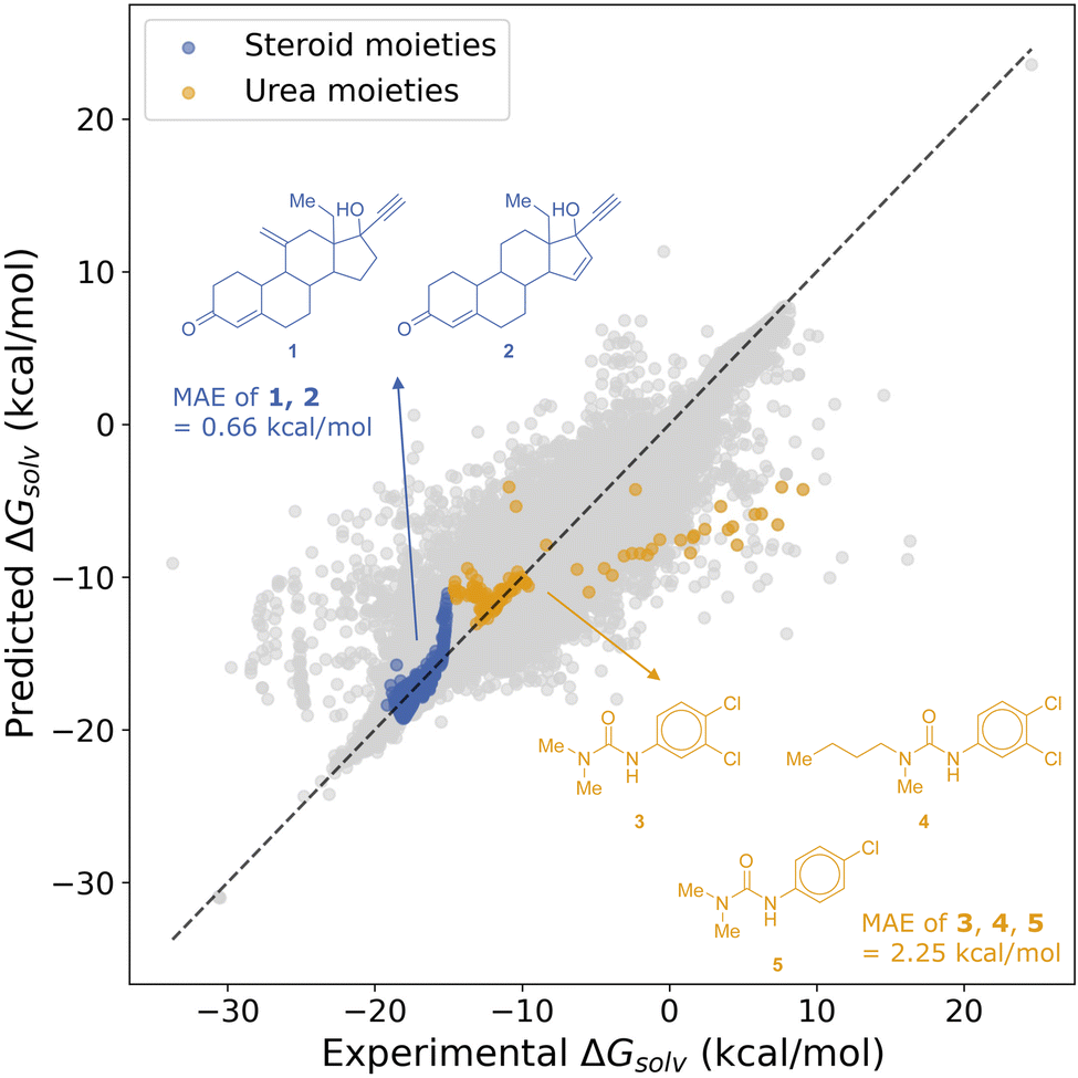
To gain deeper insight into the model's performance, we examined specific cases where predictions deviated significantly from experimental measurements in the concatenation model. Specifically, we sorted all prediction results by their absolute error and identified two distinct sets of outlier solutes emerging in different ranges of solvation free energy values. One set involved two steroid-based molecules 1 and 2, and the other consisted of urea-containing compounds 3, 4, and 5 (Fig. 6). These particular scaffolds presented greater challenges for the model, prompting further evaluation of the underlying chemical features that contributed to these prediction gaps. The first group of outliers with 1 and 2 emerged as notable outliers, with experimental solvation free energies in the range of −19 to −15 kcal mol⁻¹. Solvation free energies of these compounds dissolved in the binary solvent of water and methanol were consistently overpredicted by 5 to 7 kcal mol⁻¹ with the concatenation model. Although the introduction of the subgraph model architecture partially improved these predictions, reducing the error to about 4 kcal mol⁻¹, their accuracy remained below expectations. Interestingly, other structurally similar steroids were well predicted, suggesting that the presence of the alkynyl bond – a feature absent in any other molecules within the MixSolDB – may be driving these anomalies. This observation implies that broadening the chemical diversity of the dataset or incorporating more specialized inductive biases could further enhance predictions for such rare functional groups. On the other hand, the second group of outliers involved 3, 4, and 5 with solvation free energies ranging from 0 to 7 kcal mol⁻¹. Examples include monuron (5) dissolved in binary solvent of water and methanol, as well as its variants bearing additional chlorine substitutions and a more extended alkyl chain, dissolved in either water/methanol or water/DMSO mixtures. Solvation free energies of these urea-based molecules were systematically underpredicted by as much as 6 to 11 kcal mol⁻¹. Notably, our MixSolDB did not contain any other urea-based molecules, suggesting that the model lacked prior exposure to this chemical motif. Unlike the steroid outliers, the subgraph model architecture did not substantially reduce the prediction errors for this set. The persistent underestimation may indicate that the model struggles with certain intermolecular interactions specific to urea derivatives or that more targeted feature engineering is required to capture their distinct solvation behavior.

Fig. 6 Solutes in outlier regions with their solvation free energy values from experiments and errors in predictions.

Combining heterogeneous databases with semi-supervised distillation based on sharing weights scheme for simultaneous prediction

Outliers discussed in the previous section underscore the importance of incorporating a broader range of chemical motifs, particularly alkynyl functionalities and urea derivatives, into the model's training to achieve better generalizability. In other words, expanding the chemical space represented in the database is crucial for capturing nuanced interactions that current data curation may overlook. To facilitate such an expansion while retaining a coherent modeling framework, we implement a single GNN for solvent weight sharing, as depicted in Fig. 7A. Rather than assigning a dedicated network to each solvent, this strategy standardizes the representation process across single, binary, and ternary solvent scenarios in a unified manner. Specifically, all datapoints are treated as ternary systems, with one or two dummy solvents (e.g., “C” in SMILES representation) substituting any missing components. Although this approach introduces a modest trade-off in predictive accuracy as Fig. 7B demonstrates, it significantly increases model flexibility and applicability, allowing seamless integration of heterogeneous datasets from experimental measurements and computational generations.

Fig. 7 (A) Solvent weight-sharing schematic diagram. (B) Parity plot for our simultaneous prediction using solvent weight sharing model.

Leveraging our unified solvent weight sharing model, we further extend its generalizability and practicality by incorporating semi-supervised distillation (SSD) techniques. Given that assembling a large, fully labeled solubility database purely from experimental measurements is both challenging and resource-intensive, this framework allows us to integrate heterogeneous datasets, encompassing both experimental and computational domains, into a single training environment. In doing so, we enhance the model's predictive capabilities without the need to rely solely on an extensive, experimentally derived database. This integration of the “solvent weight sharing” model and SSD thus represents a significant step forward in creating more general, robust, and scalable solutions for solubility prediction across a wide range of chemical systems.

Many predictive models in computational chemistry are constrained by the limited availability of high-quality experimental data, while computationally generated estimates are abundantly available. To address this shortfall, we integrate a smaller but reliable experimental dataset, MixSolDB, with a much larger computationally derived dataset generated using COSMO-RS theory. COSMO-RS calculations, though comparatively easier to generate, carry inherent uncertainties due to the approximations involved in continuum solvation models. By blending these two sources, we aim to broaden the chemical space and compositional diversity captured by the model, enhancing its robustness and ability to generalize.

To build our computational dataset, we performed COSMO calculations for a large subset of molecules: 1315 solute molecules out of a total of 11 798 unique solutes and all 1445 unique solvents. These calculations yielded polarization charges for 1315 solutes and 1375 solvents. Subsequently, we generated approximately one million COSMO-RS datapoints, maintaining an even distribution among single, binary, and ternary solvent systems. For each data point, we randomly selected solute and solvent molecules from our computed pool, assigned mole fractions summing to unity, and sampled temperatures within 273 K to 373 K. The final COSMO-RS dataset comprised 998 516 datapoints: 333 062 for single solvent systems, 332 835 for binary, and 332 629 for ternary. Because our model is trained to handle single, binary, and ternary solvent systems simultaneously, it can seamlessly incorporate the newly generated COSMO-RS data. This unified training approach ensures straightforward augmentation of the dataset, allowing the model to expand its predictive domain without restructuring its architecture. However, integrating computational predictions in large quantities risks diluting data quality if all points are treated equally. To mitigate this, we employ a teacher–student SSD framework as depicted in Fig. 8. A teacher model, trained initially on the high-quality MixSolDB dataset, serves as a gatekeeper. It assigns pseudo-labels to the COSMO-RS data, accepting only those predictions that meet certain reliability thresholds. Data that fail to meet these criteria are not discarded but remain as candidates for future training cycles, providing a filtering mechanism that continually refines data quality.

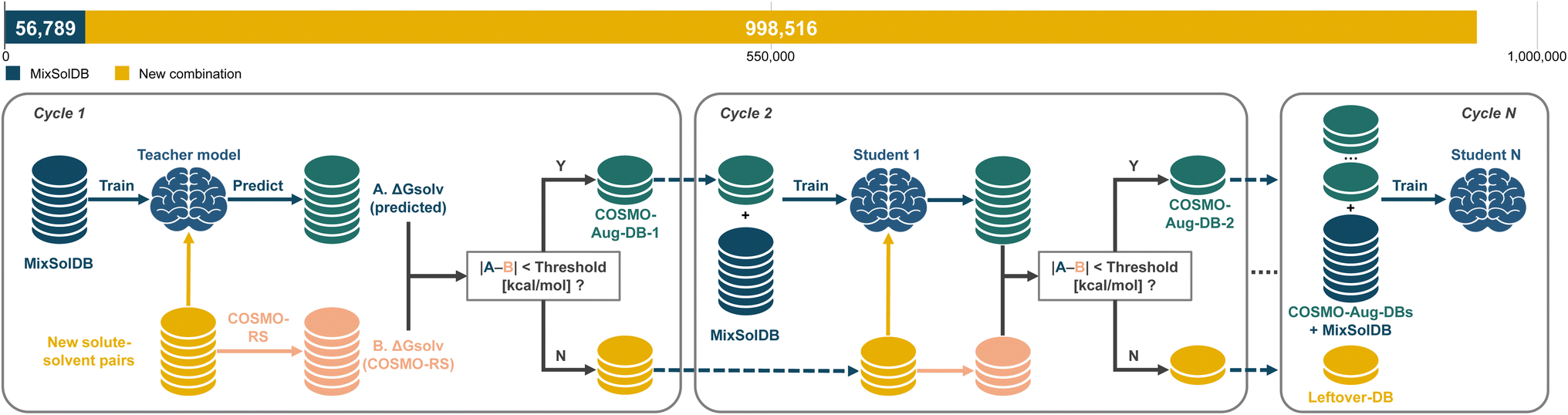Fig. 8 Schematic diagram of the semi-supervised distillation process with teacher–student framework.

We establish two threshold values colored orange and blue in Fig. 9, 0.3 and 1.0 kcal mol⁻¹, to determine whether a computational data point is sufficiently reliable to serve as a pseudo-label for the student model. The 0.3 kcal mol⁻¹ threshold is more conservative, mirroring the accuracy levels observed for carefully measured experimental data in single solvent systems. Although this strict filter preserves data quality and enhances the final predictive accuracy, it accepts fewer datapoints, potentially limiting the diversity and coverage gained. In contrast, the 1.0 kcal mol⁻¹ threshold represents a more lenient standard, still considered chemically reasonable, especially for multicomponent systems with greater complexity. This threshold admits more datapoints, broadening chemical and compositional coverage, but carries a higher risk of incorporating moderate uncertainty. Our results, visualized through violin plots in Fig. 9C, highlight the trade-offs between conservative and generous. Under the conservative 0.3 kcal mol⁻¹ threshold, the distributions of test errors remain notably tighter, as evidenced by violin plots that show comparatively narrow spreads. As shown in Fig. 9A, this stricter filtering leads to incrementally lower root mean squared error (RMSE) values, stabilizing around 1.7 kcal mol⁻¹ after successive student model iterations. However, in Fig. 9B, the cumulative number of augmented datapoints included at this threshold grows more slowly, reaching 229 917 after five SSD iterations, which is substantially fewer than the 376 026 datapoints incorporated at the 1.0 kcal mol⁻¹ threshold.

Fig. 9 (A) RMSE of SSD models based on a test set from the teacher model. (B) Accumulative size of the integrated database for each model. (C) Absolute error distribution of student models.

In contrast, models trained with the generous 1.0 kcal mol⁻¹ threshold gain access to a significantly larger dataset early on, nearly tripling the available training points after just one iteration compared to the 0.3 kcal mol⁻¹ threshold. Despite the rapid growth in data coverage, RMSE values show greater fluctuation and tend to trend higher than those from the conservative threshold, at a time exceeding 2.00 kcal mol⁻¹. The violin plots for these models confirm that the error distributions become broader, and standard deviations of absolute error are consistently higher, reflecting the introduction of noisier data. Indeed, the standard deviation measurements in Fig. 10 underscore the instability introduced by the more lenient filtering criteria, as larger portions of the computational data fail to meet stringent quality standards. In summary, lowering the threshold to 0.3 kcal mol⁻¹ ensures a more stable and accurate, yet data-limited, training environment, while raising it to 1.0 kcal mol⁻¹ dramatically expands the dataset size but at the expense of increased variability in model performance.

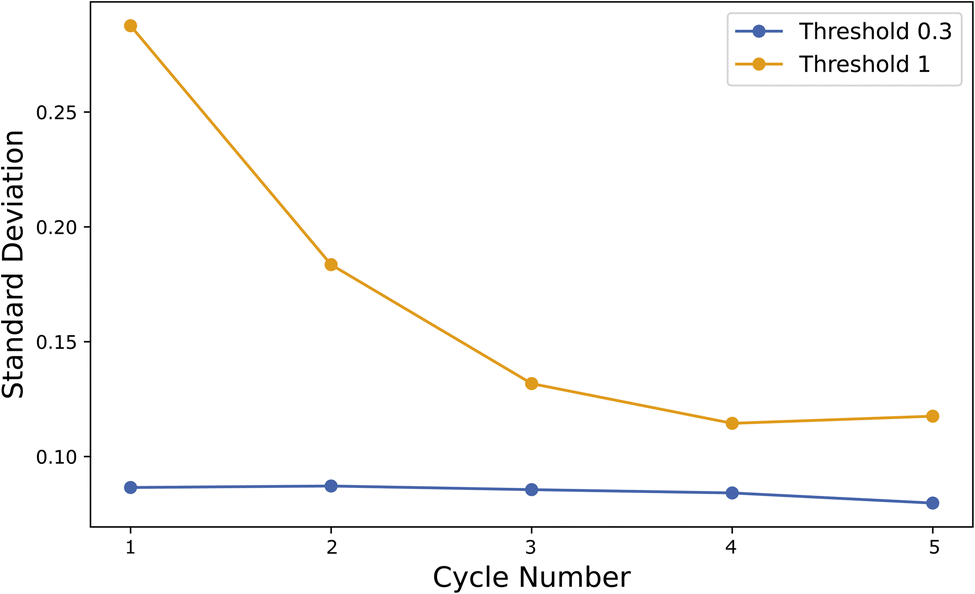Fig. 10 Standard deviation of the absolute error in augmented datapoints for each cycle in SSD.

Fig. 11 presents cluster visualizations using UMAP for three distinct scenarios related to MixSolDB and our SSD approach. Fig. 11A provides a clear depiction of the coverage within MixSolDB's chemical space, illustrating both its spread and the inherent limitations in current data representation with 56 789 entries. Fig. 11B shows 1315 solute molecules chosen for SSD procedure out of a total of 11 798 unique solutes in MixSolDB. It confirms that the solutes randomly selected for SSD constitute a reasonably broad sampling of this chemical space, ensuring that the chosen set is neither overly constrained nor unrepresentative, without any human bias. Finally, Fig. 11C demonstrates the substantial expansion of chemical space in the database following the SSD procedure at a 0.3 kcal mol⁻¹ threshold by the 5th student model with total of 229 917 datapoints. In order to represent the diverse chemical motifs present in multiple solvation system components in a single plot, we used a binary OR operation to combine the fragment identities represented by the Morgan fingerprint of each solvation system component.⁷⁴ This allows us to compactly jointly represent the chemical space covered by all molecules in each solvent–solute system. In addition to increasing coverage across diverse solvent systems (single, binary, and ternary) and temperature ranges, this expansion highlights the capacity of SSD to systematically enhance the complexity and richness of the training data, thereby pushing the boundaries of what the database can represent.

Fig. 11 (A) Cluster visualization using UMAP for MixSolDB, (B) chosen solute molecule for SSD, and (C) the database expanded after SSD.

Following these SSD procedures, we observed an increase in the number of solute molecules containing the same chemical moieties that had previously contributed to outlier behavior in MixSolDB. With this enriched chemical space shown in Fig. 12, the 5th student model trained at the 0.3 kcal mol⁻¹ threshold yielded mean absolute errors (MAEs) of 0.66 and 2.25 kcal mol⁻¹ for the first (1, 2) and second (3, 4, 5) outlier groups, respectively. Given that solvation free energies of compounds 1 and 2 in binary water–methanol mixtures were previously overpredicted by 5–7 kcal mol⁻¹ using the concatenation model, and only partially corrected to 4 kcal mol⁻¹ by the subgraph model, this improvement is significant. Similarly, for compounds 3, 4, and 5, which were underpredicted by as much as 6 to 11 kcal mol⁻¹ and not substantially corrected by the subgraph model, the decent reduction in error underscores the advantage of expanding the chemical space with SSD.

Fig. 12 Mean absolute errors (MAEs) for datapoints involving the previously discussed outlier solute molecules in MixSolDB after SSD expansion.

In conclusion, integrating MixSolDB and COSMO-RS data through SSD enables a flexible and scalable approach for solubility prediction. By adjusting threshold criteria, one can fine-tune the balance between data quality and coverage. The conservative threshold offers a meticulous filtering mechanism that maximizes predictive accuracy, while the more generous threshold accelerates the exploration of chemical space at the cost of introducing some uncertainty. This careful orchestration of datasets, thresholds, and models thus provides a robust blueprint for achieving both reliability and extensiveness in predictive models of solubility in multicomponent solvent systems.

Conclusions

In this work, we introduced and compared two graph neural network (GNN) architectures – concatenation and subgraph – for predicting the solubility of small molecules in multicomponent solvent systems. By curating a large experimental database (MixSolDB) and integrating it with computationally derived data through a semi-supervised distillation (SSD) framework, we addressed key challenges in data scarcity and model generalizability. Our results demonstrated that the subgraph GNN architecture outperformed the concatenation model in binary solvent systems, reducing mean absolute error and displaying fewer extreme outliers. We attribute these improvements to the subgraph approach's ability to capture chemically relevant interactions between solute and solvents more effectively, thus enhancing molecular representation without diluting critical information.

To further extend chemical coverage and improve predictive accuracy, we incorporated COSMO-RS calculations into the training process under a teacher–student SSD framework. By adjusting threshold criteria (0.3 or 1.0 kcal mol⁻¹) for accepting pseudo-labeled data, we balanced the trade-off between data quality and coverage, substantially increasing the diversity of solvent compositions, temperatures, and solute structures. This, in turn, produced a more versatile and scalable predictive model. Moreover, our proposed GNN-SSD framework not only demonstrated the feasibility of expanding model applicability to highly diverse solvent environments but also broadened the chemical space to address previously high error margins, particularly for challenging outlier solutes. This integration strategy further underscores how bridging experimental data with theory-based calculations can accelerate predictive accuracy in complex multicomponent systems.

Overall, these findings highlight the promise of a robust framework for achieving both coverage and precision, moving the field closer to reliable and generalizable solubility predictions that can readily be applied in a wide range of chemical contexts.

Data availability

Data for this article, including the databases and the code used for machine learning model development and training, are available at https://doi.org/10.5281/zenodo.15284975 (https://github.com/BioE-KimLab-Lab/MulticompSol).

Conflicts of interest

There are no conflicts to declare.

Acknowledgements

The authors would like to graciously acknowledge support from the Department of Chemistry at Colorado State University. This work was also supported by a National Science Foundation grant (NSF CHE-2304658). Computational resources were provided by the NSF Advanced Cyberinfrastructure Coordination Ecosystem: Services & Support program (ACCESS), Grant No. TH-CHE210034.

References

1. S. P. Pinho and E. A. Macedo, Solubility in Food, Pharmaceutical, and Cosmetic Industries, in Developments and Applications in Solubility, ed. T. M. Letcher, The Royal Society of Chemistry, 2007, ch. 20, pp. 305–322.
2. A. Jouyban, J. Pharm. Pharm. Sci., 2008, 11, 32–58.
3. A. Llinàs, R. C. Glen and J. M. Goodman, J. Chem. Inf. Model., 2008, 48, 1289–1303.
4. C. A. S. Bergström, W. N. Charman and C. J. H. Porter, Adv. Drug Delivery Rev., 2016, 101, 6–21.
5. C. A. S. Bergström and P. Larsson, Int. J. Pharm., 2018, 540, 185–193.
6. S. E. Fioressi, D. E. Bacelo, C. Rojas, J. F. Aranda and P. R. Duchowicz, Ecotoxicol. Environ. Saf., 2019, 171, 47–53.
7. A. K. Nayak and P. P. Panigrahi, ISRN Phys. Chem., 2012, 2012, 820653.
8. N. Seedher and M. Kanojia, Pharm. Dev. Technol., 2009, 14, 185–192.
9. S. A. Newmister, S. Li, M. Garcia-Borràs, J. N. Sanders, S. Yang, A. N. Lowell, F. Yu, J. L. Smith, R. M. Williams, K. N. Houk and D. H. Sherman, Nat. Chem. Biol., 2018, 14, 345–351.
10. J. Kraml, F. Hofer, A. S. Kamenik, F. Waibl, U. Kahler, M. Schauperl and K. R. Liedl, J. Chem. Inf. Model., 2020, 60, 3843–3853.
11. T. Dalton, T. Faber and F. Glorius, ACS Cent. Sci., 2021, 7, 245–261.
12. B. Steenackers, A. Neirinckx, L. De Cooman, I. Hermans and D. De Vos, ChemPhysChem, 2014, 15, 966–973.
13. T. Zhou, Z. Lyu, Z. Qi and K. Sundmacher, Chem. Eng. Sci., 2015, 137, 613–625.
14. D. Millán, J. G. Santos and E. A. Castro, J. Phys. Org. Chem., 2012, 25, 989–993.
15. A. Jalan, R. W. Ashcraft, R. H. West and W. H. Green, Annu. Rep. Prog. Chem., Sect. C: Phys. Chem., 2010, 106, 211–258.
16. P. J. Dyson and P. G. Jessop, Catal. Sci. Technol., 2016, 6, 3302–3316.
17. F. Huxoll, F. Jameel, J. Bianga, T. Seidensticker, M. Stein, G. Sadowski and D. Vogt, ACS Catal., 2021, 11, 590–594.
18. H. C. Hailes, Org. Process Res. Dev., 2007, 11, 114–120.
19. J. J. Varghese and S. H. Mushrif, React. Chem. Eng., 2019, 4, 165–206.
20. J. D. Moseley and P. M. Murray, J. Chem. Technol. Biotechnol., 2014, 89, 623–632.
21. B. L. Slakman and R. H. West, J. Phys. Org. Chem., 2019, 32, e3904.
22. J. Sherwood, H. L. Parker, K. Moonen, T. J. Farmer and A. J. Hunt, Green Chem., 2016, 18, 3990–3996.
23. X. Yang, D. Beckmann, S. Fiorenza and C. Niedermeier, Environ. Sci. Technol., 2005, 39, 7279–7286.
24. J. Esteban, A. J. Vorholt and W. Leitner, Green Chem., 2020, 22, 2097–2128.
25. G. W. Huber, J. N. Chheda, C. J. Barrett and J. A. Dumesic, Science, 2005, 308, 1446–1450.
26. Z. Shen and R. C. Van Lehn, Ind. Eng. Chem. Res., 2020, 59, 7755–7764.
27. C. A. S. Bergström and A. Avdeef, ADMET & DMPK, 2019, 7, 88–105.
28. S. Boothroyd, A. Kerridge, A. Broo, D. Buttar and J. Anwar, Phys. Chem. Chem. Phys., 2018, 20, 20981–20987.
29. R. E. Skyner, J. L. McDonagh, C. R. Groom, T. van Mourik and J. B. O. Mitchell, Phys. Chem. Chem. Phys., 2015, 17, 6174–6191.
30. J. Tomasi, B. Mennucci and R. Cammi, Chem. Rev., 2005, 105, 2999–3094.
31. J. Zhang, B. Tuguldur and D. van der Spoel, J. Chem. Inf. Model., 2015, 55, 1192–1201.
32. A. V. Marenich, C. J. Cramer and D. G. Truhlar, J. Phys. Chem. B, 2009, 113, 6378–6396.
33. J. Zhang, H. Zhang, H. T. Wu, Q. Wang and D. van der Spoel, J. Chem. Theory Comput., 2017, 13, 1034–1043.
34. Y. Takano and K. N. Houk, J. Chem. Theory Comput., 2005, 1, 70–77.
35. A. Klamt, V. Jonas, T. Bürger and J. C. W. Lohrenz, J. Phys. Chem. A, 1998, 102, 5074–5085.
36. F. Eckert and A. Klamt, AIChE J., 2002, 48, 369–385.
37. M. A. Lovette, J. Albrecht, R. S. Ananthula, F. Ricci, R. Sangodkar, M. S. Shah and S. Tomasi, Cryst. Growth Des., 2022, 22, 5239–5263.
38. A. Llinas, I. Oprisiu and A. Avdeef, J. Chem. Inf. Model., 2020, 60, 4791–4803.
39. Y. Ran, Y. He, G. Yang, J. L. H. Johnson and S. H. Yalkowsky, Chemosphere, 2002, 48, 487–509.
40. D. S. Palmer and J. B. O. Mitchell, Mol. Pharm., 2014, 11, 2962–2972.
41. S. Boobier, D. R. J. Hose, A. J. Blacker and B. N. Nguyen, Nat. Commun., 2020, 11, 5753.
42. K. Yang, K. Swanson, W. Jin, C. Coley, P. Eiden, H. Gao, A. Guzman-Perez, T. Hopper, B. Kelley, M. Mathea, A. Palmer, V. Settels, T. Jaakkola, K. Jensen and R. Barzilay, J. Chem. Inf. Model., 2019, 59, 3370–3388.
43. J. Qiu, J. Albrecht and J. Janey, Org. Process Res. Dev., 2020, 24, 2702–2708.
44. M. Lovrić, K. Pavlović, P. Žuvela, A. Spataru, B. Lučić, R. Kern and M. W. Wong, J. Chemom., 2021, 35, e3349.
45. H. Lim and Y. Jung, Chem. Sci., 2019, 10, 8306–8315.
46. Q. Cui, S. Lu, B. Ni, X. Zeng, Y. Tan, Y. D. Chen and H. Zhao, Front. Oncol., 2020, 10, 121.
47. Y. Pathak, S. Laghuvarapu, S. Mehta and U. D. Priyakumar, Proc. AAAI Conf. Artif. Intell., 2020, 34, 873–880.
48. F. H. Vermeire and W. H. Green, Chem. Eng. J., 2021, 418, 129307.
49. Y. Kim, H. Jung, S. Kumar, R. S. Paton and S. Kim, Chem. Sci., 2024, 15, 923–939.
50. J. Yu, C. Zhang, Y. Cheng, Y.-F. Yang, Y.-B. She, F. Liu, W. Su and A. Su, Digital Discovery, 2023, 2, 409–421.
51. F. H. Vermeire, Y. Chung and W. H. Green, J. Am. Chem. Soc., 2022, 144, 10785–10797.
52. C. Bilodeau, W. Jin, H. Xu, J. A. Emerson, S. Mukhopadhyay, T. H. Kalantar, T. Jaakkola, R. Barzilay and K. F. Jensen, React. Chem. Eng., 2022, 7, 297–309.
53. P. C. St. John, Y. Guan, Y. Kim, S. Kim and R. S. Paton, Nat. Commun., 2020, 11, 2328.
54. M. N. Hossain, H. C. Park and H. S. Choi, Catalysts, 2019, 9, 229.
55. M. Sharma, P. Sharma and J. N. Kim, RSC Adv., 2013, 3, 10103–10126.
56. S. M. Fakhr Hoseini, T. Tavakkoli and M. S. Hatamipour, Sep. Purif. Technol., 2009, 66, 167–170.
57. A. Hussain, M. A. Altamimi, O. Afzal, A. S. A. Altamimi, A. Ali, A. Ali, F. Martinez, M. U. M. Siddique, W. E. Acree and A. Jouyban, ACS Omega, 2022, 7, 1197–1210.
58. J. Qiu, J. Albrecht and J. Janey, Org. Process Res. Dev., 2019, 23, 1343–1351.
59. Z. Bao, G. Tom, A. Cheng, J. Watchorn, A. Aspuru-Guzik and C. Allen, J. Cheminf., 2024, 16, 117.
60. R. J. Leenhouts, N. Morgan, E. A. Ibrahim, W. H. Green and F. H. Vermeire, arXiv, 2024, preprint, arXiv:2412.01982v2,  DOI:10.48550/arXiv.2412.01982.
61. H. Jung and C. D. Stubbs, BioE-KimLab/MulticompSol: v1.0.0, Zenodo, 2025,  DOI:10.5281/zenodo.15284976.
62. A. V. Marenich, C. P. Kelly, J. D. Thompson, G. D. Hawkins, C. C. Chambers, D. J. Giesen, P. Winget, C. J. Cramer and D. G. Truhlar, Minnesota Solvation Database (MNSOL) version 2012, Retrieved from the Data Repository for the University of Minnesota, 2020,  DOI:10.13020/3eks-j0590.
63. A. Klamt and G. Schüürmann, J. Chem. Soc., Perkin Trans. 2, 1993, 799.
64. A. Klamt, J. Phys. Chem., 1996, 99, 2224.
65. COSMO-RS, https://www.3ds.com/products/biovia/cosmo-rs.
66. Y. Kim, J. Cho, N. Naser, S. Kumar, K. Jeong, R. L. McCormick, P. C. St. John and S. Kim, Proc. Combust. Inst., 2023, 39, 4969–4978.
67. J. L. Lansford, K. F. Jensen and B. C. Barnes, Propellants, Explos., Pyrotech., 2023, 48, e202200265,  DOI:10.1002/prep.202200265.
68. B. Winter, C. Winter, J. Schilling and A. Bardow, Digital Discovery, 2022, 1, 859–869.
69. E. I. Sanchez Medina, S. Linke, M. Stoll and K. Sundmacher, Digital Discovery, 2022, 1, 216–225.
70. B. Winter, C. Winter, T. Esper, J. Schilling and A. Bardow, Fluid Phase Equilib., 2023, 568, 113731.
71. H. Wang, D. Lian, Y. Zhang, L. Qin and X. Lin, arXiv, 2020, preprint, arXiv:2005.05537,  DOI:10.48550/arXiv.2005.05537.
72. S. Qin, S. Jiang, J. Li, P. Balaprakash, R. C. V. Lehn and V. M. Zavala, Digital Discovery, 2023, 2, 138–151.
73. K. He, X. Zhang, S. Ren and J. Sun, Proc. IEEE Conf. CVPR, 2016, pp. 770–778.
74. Y. Kim, S. Kumar, J. Cho, N. Naser, W. Ko, P. C. St. John, R. L. McCormick and S. Kim, SAE Technical Paper, 2023.

---

Footnotes

† Electronic supplementary information (ESI) available. See DOI: https://doi.org/10.1039/d5dd00015g

‡ Equal contribution.

---