Predicting hydrogen atom transfer energy barriers using Gaussian process regression

Abstract

Predicting reaction barriers for arbitrary configurations based on only a limited set of density functional theory (DFT) calculations would render the design of catalysts or the simulation of reactions within complex materials highly efficient. We here propose Gaussian process regression (GPR) as a method of choice if DFT calculations are limited to hundreds or thousands of barrier calculations. For the case of hydrogen atom transfer in proteins, an important reaction in chemistry and biology, we obtain a mean absolute error of 3.23 kcal mol⁻¹ for the range of barriers in the data set using SOAP descriptors and similar values using the marginalized graph kernel. Thus, the two GPR models can robustly estimate reaction barriers within the large chemical and conformational space of proteins. Their predictive power is comparable to a graph neural network-based model, and GPR even outcompetes the latter in the low data regime. We propose GPR as a valuable tool for an approximate but data-efficient model of chemical reactivity in a complex and highly variable environment.

---

1 Introduction

Chemical reactivity in complex chemical or biochemical systems can be assessed typically at very high accuracy using quantum chemical methods such as density functional theory (DFT). Surrogate models built using machine learning have been recently suggested to be able to replace these computationally demanding DFT calculations.¹ The trained model serves as a black box approximation of the true mapping between reaction geometries and energy barriers. Machine-learned surrogate models can in principle predict reaction barriers solely based on molecular structures, after being trained on pre-calculated DFT barriers, albeit at lower accuracy than the actual DFT calculation itself.^2,3

In molecular machine learning, graph representations for molecular prediction problems have seen great success in recent years, specifically in the form of Graph Neural Networks (GNNs). Prominent recent examples include the frameworks Polarizable Atom Interaction Neural Network (PaiNN),⁴ Neural Equivariant Interatomic Potentials (NequIP)⁵ and MACE.⁶ We have recently shown that a variant of the PaiNN model can be used to predict electronic activation energies, in this paper referred to as energy barriers, of hydrogen atom transfer (HAT) reactions in proteins.⁷ We have chosen HAT because of its important role in proteins subjected to oxidative stress molecules, light, or, as recently shown by us, mechanical force. Mechanoradicals are formed in type I collagen through homolytic bond scission when subject to mechanical stress.⁸ The generated radicals migrate through the material, eventually to a site that can stabilize radicals.⁹ Understanding the mechanisms behind these reactions is especially interesting to get a better insight into the effects stress, such as exercise, can have on protein materials like collagen. Beyond mechanoradicals, migration of protein radicals, originating from light, oxidative stress molecules, or other external factors, often occurs through HAT, e.g. ref. 10. Exact radical migration paths are, however, mostly unknown. This renders HAT an interesting test bed to tackle the prediction of biochemical reactivity.

Our model presented in ref. 7 based on PaiNN was able to predict HAT reactions with geometries obtained from molecular dynamics (MD) simulations, with a mean absolute error (MAE) of 2.4 kcal mol⁻¹ when restricting the prediction to transitions with distances ≤2 Å, i.e. the most relevant transitions in a material.

Geometries originated directly from molecular dynamics (MD) simulations, without subsequent DFT optimizations, rendering such a method very efficient. The model allows the prediction of a reaction barrier for virtually any reactant pair occurring during an MD simulation of the protein. This can ultimately allow simulating these reactions in a kinetic Monte Carlo setting coupled to the MD simulations, i.e. reactive dynamics of the biochemical system under investigation.¹¹ From a practical perspective, the energy barrier prediction should only rely on the initial geometric configuration as input for it to be useful in a future application.

One major drawback of building such a surrogate model is the need to initially compute, using DFT, a large set of energy barriers of the reaction at hand to train the model. Here, large often refers to thousands of barriers, in our case to 19 164 barriers for reaching an intermediate accuracy of a PaiNN model for HAT, with further room for improvement by enlarging the dataset. For practitioners, a more data-efficient model would be very advantageous.

We propose two alternative variants to model these reactions with Gaussian Process Regression (GPR):¹² (1) using the Smooth Overlap of Atomic Positions (SOAP) descriptor¹³ and (2) using the Marginalized Graph Kernel.^14–17 We show that these approaches are a useful alternative to the previously developed GNN, especially in the low data regime. This is of particular interest, since DFT can be very computationally demanding for large systems at high levels of accuracy. Therefore, acquiring new training points can be costly. The proposed methods would allow practitioners to achieve good predictions while reducing the time and cost spent generating training data.

2 Methods

2.1 Data

For the predictions, we used the same data as obtained and described in ref. 7. In short, the data was generated in two ways. The first method consisted mostly of procedurally positioning two amino acids such that two hydrogen atoms faced one another, after which a random distance and tilt angle between the amino acid pairs was chosen and one of the hydrogen atoms was removed to represent a radical centre. Also, intramolecular transitions were considered, in which the acceptor and donor of the hydrogen atom reside in the same molecule. The data generated via this method will, in agreement with ref. 7, be referred to as synthetic systems. In contrast to this, the trajectory systems were taken as sub-systems from molecular dynamics trajectories, where possible HAT reactions were first identified. After removing duplicate transitions as well as a clear outlier, the training set consisted of 17 238 energy barriers and 1926 randomly chosen barriers as the test set. The hydrogen atom was moved from initial to end position in a straight line, see Fig. 1a, and DFT energies were obtained at equidistant steps along the transition as can be seen in Fig. 1b. Note that DFT values for steps 1, 2, 8, and 9, as depicted in Fig. 1a and b, were often not calculated, since the transition state was found to be mostly around the geometric middle (see ref. 7). We define the energy barrier ΔE as the difference between the maximum and the initial DFT calculated energy of a given reaction geometry and direction.

Fig. 1 Predictive modelling of hydrogen atom transfer energy barriers by GPR. (a) Projection of the HAT reaction for a given geometry. The hydrogen atom moves in a linear trajectory at equidistant steps. All other atoms remain fixed. (b) The energy of the system is calculated using DFT for each step of the transition. The energy barrier is taken as the difference between the maximum and initial energy. (c) For the SOAP method, the SOAP vectors were centred on the initial position (S), the final position (E) and the halfway point (M).

As discussed in ref. 7, a linear transition path is a reasonable estimate of the true reaction. Nonetheless, this neglects that neighbouring atoms can undergo conformational changes during the reaction. Therefore, some structures in the dataset were additionally optimized using the same level of DFT as the energy calculations. This is computationally more expensive, but also yields more realistic energy barriers. In total, 1434 optimized reaction barriers were used for training and 162 barriers as a randomly selected test set.

It is important to note that each transition, both optimized and not optimized, has two energy barriers, namely, one for each direction of the transition.

2.2 Gaussian process regression

In this paper, we use Gaussian Process Regression (GPR),¹² a flexible and probabilistic machine learning method, to predict energy barriers of HAT reactions. For the purpose of conciseness, we here only introduce the necessary equations. The ESI, Section A,† includes a more complete description of GPR and the used definitions. In short, our GPR models a collection of m unobserved scalar values Y_u using a collection of n observed scalar values Y_o by assuming that the union of Y_u and Y_o, denoted as Y, follow a multivariate normal distribution (MVN) with a covariance structure given by the following parametric function:

K_θ(x,x′) = σ²(C_θc(x,x′) + g²δ_x,x′), (1)

where C_θc(·,·) is any valid class of correlation functions, which can be characterized by the set of parameters θ_c, x and x′ are covariates, g ≥ 0 is the nugget term that models the potential white noise of the data, σ > 0 models the process standard deviation, and θ = (θ_c,σ,g) embodies the complete set of parameters found in the defined covariance function. The (i,j)th element of the covariance matrix Σ of the MVN is given by K_θ(x_i,x_j). Furthermore, we here assume that the MVN has a constant mean value μ.

It is therefore possible to condition the MVN on the observed values Y_o, yielding a different (conditional) MVN of the unobserved values Y_u. The resulting MVN is specified by the following mean vector and covariance matrix:

μ_u|o = μ + Σ_uoΣ_oo⁻¹(Y_o − μ) (2)

Σ_u|o = Σ_uu − Σ_uoΣ_oo⁻¹Σ^⊤_uo, (3)

where Σ_IJ is the covariance matrix block corresponding to rows I and columns J in the original joint Σ. The variance or the uncertainty of the unobserved points is given by the diagonal elements of (3). We estimate μ using the mean of Y_o.

Evidently, the GPR based predictions from (2) and (3) rely on the specified mean μ, which in general need not be a constant, and the covariance function K_θ(·,·). The covariance function serves as a robust mathematical metric for determining “similarity” among samples, under the premise that the most “similar” samples have the most influence on the outcome. Selecting an appropriate covariance function is critical for making high-quality predictions.

Furthermore, once the covariance function is selected, it is necessary to estimate its associated parameters, denoted by θ, so that they align well with the observed data. Maximum likelihood estimation (MLE) is commonly employed for this task in GPR. However, the computational cost and time complexity of MLE can become prohibitive for large n, leading to the use of approximate methods. Among these, methods based on composite likelihoods¹⁸ are quite common. In this work, we specifically use a particular variant of composite likelihood called random composite likelihood estimation.¹⁹ In the following sections, we explore the two distinct definitions of the covariate x and correlation function C_θc(·,·) in our study, resulting in two different GPR models.

2.3 Smooth overlap of atomic positions method

Given that GPR modelling of the HAT reaction necessitates the covariance functions to accurately capture reactions related to atomic geometries, constructing an accurate covariance function that represents the specifics of the HAT setting is not straightforward. This is particularly challenging since most common kernels primarily rely on real-valued scalars as features.

Smooth Overlap of Atomic Positions (SOAP)¹³ is an elegant representation of a local atomic environment. Consider an atomic environment that is centred on an atom and extends up to a cut-off radius r_cut. Let the atomic density be the sum of atoms inside this environment, where each atom is transformed into a Gaussian density. The atomic density of atoms of chemical species a is then given by²⁰

where ρ_a(r) is the atomic density at position r with the coordinate system fixed on the central atom, σ_S is the length scale parameter of the Gaussian smearing, r_i is the centre of atom i, the sum runs over all neighbours of species a of which there are N_a in total. The function f_cut decreases smoothly towards 0 as the argument approaches r_cut. The atomic density can be expanded in terms of spherical harmonics and orthogonal normalized radial basis functions g_n, such that , where c_anlm are expansion coefficients that can be calculated. In real-world applications, the infinite sum is truncated at some predefined maximum values n_max and l_max.

The SOAP power spectrum can be defined as

which can be collected as individual components of a vector and is invariant under rotation, permutation, and translation,²⁰ here referred to as the SOAP vector of an environment.

In order to model the HAT process, a covariance function needs to be defined where similar atomic geometries result in a high correlation and vice versa. It has been shown in previous works that the starting environment as well as the transition state environment are important in predicting energy barriers in HAT reactions.²¹ For this method we choose a correlation function in the following way,

where x = (x_S, x_M, x_E, x_d) and x′ represent two different reactions, and the subscripts S, M and E stand for the SOAP vectors of the environments at steps S (initial position), M (halfway point) and E (final position), respectively. The feature x_d stores the total transition distance, since this was previously found to correlate with the energy barrier.⁷ The parameters θ_c = (λ_S, λ_M, λ_E, λ_d) of each feature refer to the respective positive valued length-scale of the difference of the feature vectors.

Eqn (6) is equivalent to a product of squared exponential correlation functions¹² which is a valid kernel as a result of the Schur product theorem.²² We considered also including SOAP environments at other steps of a transition, however we found that this only marginally improved the results, but required a much higher computational cost. The interpretation of this kernel suggests that reactions, where the beginning, intermediate, and final environments, along with the total transition distance, exhibit similarity, should correspondingly produce similar energy barriers. Conversely, if any of these features demonstrates dissimilarity, it would result in a minor contribution to the prediction.

We placed a hydrogen atom at the starting, middle, and end positions of the HAT reaction. Each of these hydrogen atoms was assigned a different unique chemical species, since SOAP does not interpret the chemical elements, but instead only serves to distinguish geometrically the hydrogen atom at each step of the transition from the other atoms. The environments around the starting, middle and end positions were encoded as SOAP vectors as depicted in Fig. 1c. Through manual trial and error optimization of randomly chosen validation sets from the training set, we chose the SOAP parameters as r_cut = 2.5 Å, σ_S = 0.3 Å, n_max = 12 and l_max = 12. The SOAP vectors were calculated using the DScribe library²³ and normalized. Furthermore, the energy barriers and transition distances were standardized during training using their respective training means and standard deviations.

2.4 Marginalized graph kernel

As an alternative to using descriptors to capture the geometries of the transition, we built a GPR model using graphs. Here we define a graph G as a set of vertices V = {v_i}_i=1…N, where some vertices are connected through undirected edges E = {e_ij}_i,j=1…N with associated weights w_ij. The Marginalized Graph Kernel (MGK) was first introduced in ref. 14 and computes the covariance between two graphs by comparing random walks on each graph. Following the explanation and notation of ref. 15, the MGK covariance is the expectation value of the covariance between all possible concurrent random walk paths on the two graphs. Each vertex v_i has a start probability p_s(v_i) for the walk to begin at this vertex and, similarly, a termination probability p_e(v_i). The weight w_ij of an edge e_ij, obtained through a separately defined function, the adjacency rule, is used to calculate the transition probability , where the sum runs over all vertices connected to vertex v_i. Let h = (h₁, h₂, …, h_l) be a vector recording the vertex path resulting from the chain of length l. The MGK between graphs G and G′ can then be written aswhere K_V and K_E are covariance functions that compare the labels of two vertices or edges, respectively. Eqn (7) can be rewritten as a system of linear equations¹⁴ and solved efficiently on a modern GPU as implemented in the library GraphDot.^15,16

For each HAT transition we construct one graph. An example of such a construction is illustrated in Fig. 2a. We place a hydrogen atom at the start, end, and mid-point of the transition, as was done for the SOAP method, and similarly each of these hydrogen atoms is assigned a unique special value s_v. All other atoms are assigned a different special value to differentiate between the hydrogen atom involved in the reaction and all other atoms. In order to create an artificial feature that smoothly distinguishes between atoms on the donor and acceptor side of the reaction, we take the dot product between the normalized transition direction vector and the unit vector from the atom to the midpoint of the transition path,

where r_i is the position vector of atom i, and r_S, r_M, and r_E are the position vectors of the transition hydrogen atoms that were placed at the start position, midpoint, and end position, respectively. We found that adding this feature noticeably improved the predictions.

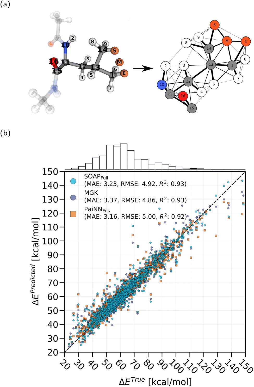Fig. 2 (a) Example of a reaction converted to a graph used for the Marginalized Graph Kernel. Semi-transparent atoms are beyond the considered threshold distance from the transition and therefore ignored. Edge thickness indicates the weight and is not to scale. (b) Final predictions for all trajectory test data using the SOAP method trained on the entire training data set as well as the MGK method. For comparison we also show predictions of a PaiNN ensemble model. We indicate the MAE, root-mean-square error (RMSE), and coefficient of determination (R²) of the test set.

For the vertex kernel we chose

K_V(v,v′) = δ(a_v,a_v′; 0.7)δ(s_v,s_v′; 0.2)exp(−|ξ_v − ξ_v′|/2), (9)

where v and v′ are vertices in graph G and G′, respectively, a_v is the atomic number, and s_v is the special type of atom or vertex v. The Kronecker delta function δ is defined aswhich follows the proposed form given in ref. 15. We chose the edge kernel aswhere e and e′ are two edges connecting atoms in graphs G and G′, respectively, d_e is the distance between atoms in angstrom that are connected through e, and λ_D is the length-scale parameter which was set to 1.0 Å. We used the adjacency rule proposed in ref. 15 which utilizes a Gaussian to calculate the edge weights based on the typical bond lengths. The weight used for each edge was computed usingwhere r_i and r_j are the positions of atoms i and j, γ_ij is the typical bond length of the elements of the two atoms given in ref. 15, and β is a scaling parameter, which was set to 1.0. This means that random walkers mostly traverse over edges which are close to classical chemical bonds, but have a small non-zero chance to sample other edges. Edges that were longer than 3 Å were removed to reduce computational cost, with the exceptions of the transition hydrogen atoms, which were always connected. All random walks were set to start on one of the hydrogen atoms involved in the reaction, namely S, M, or E. The termination probability p_e was set to 0.05 for all vertices in a given graph. Lastly, we removed all atoms which were further than 5 Å from the initial position, midway point, or end position. This was done to mimic the expected strong locality of the HAT process.The parameters of the kernels were chosen through manual trial and error on randomly sampled validation sets. We used the GraphDot¹⁵ library for the calculation of the MGK covariance matrix. Due to the large number of training points, the MGK covariance matrix was constructed blockwise in parallel using multiple GPUs. Afterwards, the normalized MGK covariance matrix was inserted into (1) in place of the correlation function and subsequently, the parameters g and σ were found using the aforementioned approximate MLE method.

2.5 Uncertainty quantification

An advantage of using GPR is that the predictions are probabilistic and therefore allow for straight-forward uncertainty quantification. Uncertainty is here quantified using a predictive probability distribution of the energy barrier given a new input geometry. A commonly employed principle in judging probabilistic predictions is that a predictive distribution should achieve maximal sharpness while still being calibrated.²⁴ Here sharpness refers to the concentration of the predictive distribution and calibration is a measure of the statistical compatibility of predicted and true values.

A simple tool for assessing the calibration of predictive distributions is the probability integral transform (PIT).^24–26 Let F_i be the predicted cumulative distribution function (CDF) for input i. We can then compute the probability that a measurement will be smaller or equal to the true value Y_trueⁱ through

p_i = F_i(Y_trueⁱ). (13)

If F_i is the true CDF, then p_i will have a standard uniform distribution. By plotting the histogram of the p_i values, systematic effects can be recognized. Note that the uniformity of the PIT histogram is a necessary, but not sufficient condition for well-calibrated predictive distributions as discussed extensively in ref. 24.

Proper scoring rules²⁷ can be utilized to simultaneously assess calibration and sharpness by assigning a score to the pair of true observation and the corresponding predictive distribution. A score is called proper, if, in expectation, the best score is achieved by the true probability distribution of the data-generating process. Here we use the convention that a lower score indicates a better prediction distribution and therefore allows a direct comparison between different methods. A commonly employed proper scoring rule is the negatively oriented logarithmic score (LogS),²⁷

LogS(f_i,Y_trueⁱ) = −log(f_i(Y_trueⁱ)), (14)

where f_i is the probability density function of the CDF F_i and Y_trueⁱ is the true value for some test point i. Another common proper scoring rule is the negatively oriented continuous ranked probability score (CRPS),²⁷where 1[c] is the indicator function, which is 1 if c = True and 0 otherwise. The CRPS has the same unit as Y, and for point predictions simplifies to the absolute error.²⁷ In this paper, we make use of the closed form expressions of the CRPS for the Gaussian distribution²⁸ and the Student's t-distribution.²⁹ Instead of assessing the entire predictive probability distribution, it is also possible to score predictive intervals. We consider a central prediction interval (PI) which quantifies a range in which a future measurement is likely to fall with probability (1 − α) × 100% with lower and upper bounds of quantiles at level α/2 and 1 − α/2, respectively. A popular scoring rule to evaluate the quality of a predicted PI is the negatively oriented Interval Score (IS)²⁷where a is the lower limit of the PI, and b is the upper limit. For all scoring rules, we calculate the mean score over all predictions. For the GPR methods, we utilized the predicted Gaussian variance given in 3 to calculate the PI boundaries for a given α value.

In the case of the PaiNN models, we construct the predictive intervals and distributions similar to ref. 30, which assumes that the bias is sufficiently negligible and that the point predictions of the models are Gaussian distributed around the true value. We neglect noise effects and construct the lower and higher bounds of the prediction intervals for the point i as

[[small mu, Greek, circumflex]_i − c(α/2)[small sigma, Greek, circumflex]_i, [small mu, Greek, circumflex]_i + c(α/2)[small sigma, Greek, circumflex]_i], (17)

where [small mu, Greek, circumflex]_i is the ensemble mean, [small mu, Greek, circumflex]_i is the ensemble sample standard deviation and c(·) is the quantile function of the Student's t-distribution. For the calculation of the LogS and CRPS, we used the Student's t-distribution with degree of freedom 10, the number of ensemble members, together with the ensemble sample mean and standard deviation as the predictive distribution. Following ref. 30, by using the above construction, we would obtain confidence rather than prediction intervals, the latter of which, in this framework, is expected to be larger due to inherent random noise. However, in our case, the PaiNN model learns from the full spatial and atomic type information which is equivalent to the input used for the deterministic DFT calculations, and therefore it can be argued that additional modelling of noise is not necessary. Nonetheless, a more extended analysis of the implications is needed and left to future work.

3 Results and discussion

3.1 Predictions

We trained two models based on SOAP and MGK, respectively, as described in the Methods section, using 17 238 HAT barriers from DFT calculations, comprising both synthetic (7884 barriers) and trajectory data (9354 barriers). The MLE optimization procedure of the SOAP method yielded the final mean kernel parameters: λ_S = 2.1, λ_M = 1.8, λ_E = 3.3, λ_d = 3.4, σ = 1.3 and g = 0.1. The nugget g was always initialized close to 0.1, since it was observed that this stabilized the optimization procedure. We tested the two models on 1044 HAT barriers from trajectory data and found an overall MAE of 3.23 kcal mol⁻¹. We signify this type of trained model, where the training set included both synthetic and trajectory barriers, with SOAP_Full. For the MGK method, we found through MLE g = 0.02 and σ = 7.7 using all barriers for training. The MAE was found to be 3.37 kcal mol⁻¹, resulting in a slightly worse performance than the SOAP-based method.

For the SOAP method, we additionally trained a model only using the trajectory data, referred to as SOAP_Traj, resulting in: λ_S = 5.7, λ_M = 2.8, λ_E = 10.4, λ_d = 8.2 Å, σ = 3.8 and g = 0.06 with an average MAE of 3.26 kcal mol⁻¹. The MAE is very similar compared to the model using all training data, even though it only used ≈54% of all data. This indicates that for the purpose of predicting in a trajectory setting, the synthetic data appears to only marginally improve the predictions.

Fig. 2b shows the energy barrier prediction results of the SOAP and MGK methods for all trajectory test data trained using both synthetic and trajectory data. For comparison, we also include the ensemble predictions of a PaiNN ensemble model, as described in ref. 7, which we trained on the same data. The ensemble model, referred to as PaiNN_Ens, consisted of the mean prediction of 10 individually trained PaiNN models, which are here referred to as PaiNN_Ind. Note that each ensemble member was trained on randomly sampled 90% of the training data, with the rest used for validation. Overall, the SOAP method can be seen to slightly outperform the MGK method. There are only few outliers, and most test points form a narrow band around the diagonal. The error tends to be much higher for large barriers, which can be attributed to the low number of training points in this range. In practice, these points are not very relevant, since the transitions are very unlikely to occur. It is particularly interesting to note that some outliers form close triplets, where the prediction error of all three methods is very similar. This suggests that, for these geometries at least, all methods must have some similarity in the way they make predictions. This is remarkable, since superficially the three methods capture the reactions in very different ways.

The test MAE results for the different methods are summarized in Table 1. We also include the performance for reactions where the transition distance d is smaller or equal to 2 Å or 3 Å, focusing on reactions that have typically lower barriers and are therefore more relevant in a protein environment, as discussed in ref. 7. Remarkably, both GPR-based models perform nearly as well as the previously suggested graph neural network (PaiNN) ensemble model⁷ with the MAE of the test set only sightly larger. We show in the next section that this can be directly related to the data efficiency of the GPR and GNN method.

Table 1 Test MAE in kcal mol⁻¹ for all trajectory data (top row) or if only including transitions with a maximum transition distance d (bottom two rows)

Test set	SOAPFull	SOAPTraj	MGK	PaiNNInd	PaiNNEns
All (no cut-off)	3.23	3.26	3.37	3.55	3.16
Cut-off d ≤ 3 Å	3.08	3.11	3.20	3.30	2.94
Cut-off d ≤ 2 Å	2.79	2.82	2.85	2.83	2.53

---

3.2 Data efficiency

A major drawback of training on DFT calculated data is that constructing the training set can be very computationally demanding. It has been observed previously, e.g. see ref. 1 and 3, that GPR can be more data efficient than a similar neural network approach. Here we compare the data efficiency of the GPR SOAP-based method with the PaiNN GNN. The average and standard deviation of the MAE results for different training set sizes can be seen in Fig. 3. For the SOAP methods, a training subset was randomly sampled from the entire training set with 8 different initial seeds, and the subsequent MLE parameter estimation was performed on these subsets. This was similar for the PaiNN models, however additionally for each training seed, 10 models were trained. All of these individually trained PaiNN models will be referred to as PaiNN_Ind. The 10 PaiNN_Ind with the same seed, constituted one ensemble model PaiNN_Ens, such that there were 8 ensemble GNNs for a given training set size. The error bars signify the sample standard deviation of the MAE over multiple runs. Occasionally, the optimization procedure found suboptimal parameters for a run, as can be observed in the noticeably larger spread and mean for SOAP_Full at 10% of the total training size. We find that in the low to mid-data regime, i.e. low-hundreds to mid-thousands of data points, GPR clearly outperforms the individual GNN models as well as the derived ensemble models. With increasing training size, the MAE of the GNN and GPR method converge, after which the ensemble GNN method achieves overall a lower MAE. After observing that the training curves appear linear on a log–log scale, we fit a power law to the results, in the form of

ε = a·n_train^k, (18)

where ε is the MAE, n_train is the number of training points used, a is a fitting parameter and k represents the fitted slope of the learning curve on a log–log scale. The fitting was performed using SciPy's³¹ non-linear weighted least squares implementation with (18). The results are shown in Table 2. Additionally, we estimate the number of training points n_threshold which would be required to reach a target MAE of 2 kcal mol⁻¹, if the fitted power-law relations were to hold for larger training set sizes. We find that the GNN methods would be expected to reach this threshold with significantly fewer training points, approximately ×4.3 the number used here. Lastly, we calculated the intersection of the fitted models for the SOAP_Full and PaiNN_Ens case and find that an equal MAE would be achieved for 7000, 10 000 and 13 000 number of training points in the case of transitions with d ≤ 2 Å, 3 Å, or all transition distances considered in the test set, respectively.

Fig. 3 Test MAE for the SOAP GPR and PaiNN methods studied using different fractions of the total training data for transition distances ≤3 Å and ≤2 Å respectively.

Table 2 Fitted parameters of (18) for different prediction methods for all trajectory transitions. We extrapolate which training set size would be required to achieve an MAE of 2 kcal mol⁻¹ on the entire trajectory dataset

Method	a [kcal mol^−1]	k	n threshold
SOAPFull	22.6	−0.20	190 × 10^3
SOAPTraj	18.3	−0.19	126 × 10^3
PaiNNInd	69.5	−0.31	105 × 10^3
PaiNNEns	62.5	−0.31	74 × 10^3

---

3.3 Uncertainty quantification

In Fig. 4a we show the PI accuracy plot,^32,33 where we calculate the empirical coverage, i.e. the fraction of predictions that are found inside the respective central prediction interval. Overall it can be seen that the PaiNN ensemble method substantially underestimates the intervals while the SOAP methods is too conservative and chooses intervals that are larger than necessary.

Fig. 4 Predicted vs. empirical coverage (a) and the probability integral transform (b). Both figures were evaluated on all trajectory test data.

Similar conclusions can be drawn from Fig. 4b which shows the PIT distribution for all three methods. The GPR methods exhibit a hump-like shape, indicating overdispersion, meaning that the predictive distributions are too wide and fewer values are found in the tails than expected. In stark contrast, the PIT of the PaiNN ensemble is clearly U-shaped, i.e. underdispersed, suggesting that far more values are found in the tails than expected and that the distributions are too narrow. Fortunately, no clear triangular slopes can be observed, which would otherwise be an indication of bias.²⁴ A simple possibility to improve the calibration of both methods would be to find an optimal factor that linearly scales the standard deviation using a separate validation data set,^20,27 which we leave to future work.

Prediction intervals at levels close to 100% are most interesting, since by definition they promise to capture the true observations with a very high probability. Table 3 shows the arithmetic mean over 8 runs of the mean IS for PIs of different sizes. It can be seen that while at the level of 50% the PaiNN ensemble model appears to score marginally better, the SOAP methods clearly outperform the ensemble method at high level probability prediction intervals. This indicates that the SOAP GPR models are better suited than the PaiNN ensemble method, if one wishes to define ranges that should contain a future observation with a high probability.

Table 3 Arithmetic mean of the average interval score over 8 runs in kcal mol⁻¹

Prediction interval	SOAPFull	SOAPTraj	PaiNNEns
50%	11.6	11.2	10.8
80%	19.0	17.8	18.2
90%	24.3	22.8	26.2
95%	29.8	28.3	38.1
99%	46.6	47.9	95.9

---

Table 4 shows the CRPS and LogS values for the different models when using all available training data (in case of the SOAP_Traj this means only trajectory training data), or only 860 training points, which corresponds to 5% of all training data. When using all training data, the results are inconclusive, since the PaiNN ensemble method marginally outperforms the GPR models using the CRPS scoring rule, but is outperformed under the LogS score. However, when using only a limited amount of data, here only 860 training points, the GPR methods clearly achieve better CRPS and LogS values. Therefore, in the low data regime, the predictive distributions of the GPR models should be favoured over the PaiNN ensemble method.

Table 4 Arithmetic mean over 8 runs of the CRPS in kcal mol⁻¹ and LogS values for the different methods using either all the available training data (in case of SOAP_Traj this only includes trajectory data) or only 860 training points

Scoring rule	SOAPFull	SOAPTraj	PaiNNEns
CRPS (All data)	2.55	2.48	2.45
CRPS (5% of all)	4.24	3.72	5.91
LogS (all data)	2.99	2.96	3.12
LogS (5% of all)	3.42	3.28	4.22

---

3.4 Optimized energy barriers

The energy barriers of the optimized reactions, that is, energy differences between optimized transition states and reactants, can be expected to be closer to the true energy barriers compared to the unoptimized reactions. There are only few optimized energy barriers due to the substantial computation cost. Therefore, learning on these directly is expected to be very inefficient, even for the more data-efficient GPR.

We choose to model the optimized energy barrier as the unoptimized case with an additional correction term, namely as

ΔE_optimized(x) = ΔE_unoptimized(x) + δ(x), (19)

where x is some HAT reaction, ΔE_optimized is the energy barrier after optimization of reactants and transition state, ΔE_unoptimized is the energy barrier without structure optimization, and δ(x) is the correction term. We showed in the previous sections that the GPR method performs better in the low data regime, and the GNN achieves better results when more training data is available. We therefore hypothesized that the GPR method is better suited to learn δ(x), since there are significantly fewer optimized energy barriers available, namely, 1434 training barriers and 144 test trajectory barriers. By using the ensemble GNN method to predict ΔE_unoptimized(x) we take advantage of this method's strong performance when utilizing all unoptimized training data.

The GPR SOAP method was used to train on the difference between ΔE_optimized and the predicted values of ΔE_unoptimized of a retrained PaiNN_Ens model, which did not include these reactions in its training set. The MAE for the trajectory test set was found to be 4.55(13) kcal mol⁻¹ and 3.77(15) kcal mol⁻¹ with distances d ≤ 3 Å and d ≤ 2 Å respectively, where the results indicate the mean and standard deviation of 8 independent PaiNN and subsequent GPR runs. This is a slight improvement on the previous state-of-the-art results reported in ref. 7 as 4.93 kcal mol⁻¹ for the d ≤ 3 Å case by around 7.8% and comparable to the result of d ≤ 2 Å which was found to be 3.64 kcal mol⁻¹.

4 Conclusions

Gaussian Process Regression (GPR) models are capable of predicting reaction barriers of Hydrogen Atom Transfer (HAT) reactions and their performance almost reaches that achieved by modern Graph Neural Network (GNN) models for the full training set and clearly outperforms the latter in the low data regime.

The performance of the GPR models proposed here is similar for two vastly different kernels used, one based on Smooth Overlap of Atomic Positions (SOAP) descriptors and the other employing the marginalized graph kernel. As the major advantage of GPR over GNNs, we find the kernel method to be highly data-efficient, outperforming the GNN for sample sizes of thousands of density functional theory (DFT) energies or smaller. We thus propose GPR to be a method of choice if predictions are needed without the availability of large amounts of data, e.g. for a first screening of a large chemical space of a reaction. Additionally, we envision that an active learning³⁴ approach could be used, where the training set is built iteratively by including candidate transitions with the smallest predicted barriers to increase efficiency in sampling the most relevant reactions.

We estimate that 4.3 times the data would be needed to achieve a target accuracy of 2 kcal mol⁻¹ for the unoptimized barriers in the case of the best-performing GNN ensemble method, under the assumption of a continued power law behaviour. We showed that by combining the strengths of the GNN method, i.e. overall best performance for the unoptimized barriers, and the GPR method, namely, data efficiency, we achieve an improved mean absolute error (MAE) for the optimized energy barriers on this dataset for transition distances d ≤ 3 Å. Furthermore, we showed that the SOAP-based GPR method achieves a better interval score for prediction intervals for the ≥80% range, indicating that GPR is better suited for uncertainty quantification in this range. The SOAP GPR methods achieve noticeably better logarithmic score (LogS) and continuous ranked probability score (CRPS) values than the GNN ensemble methods in the low data regime. However, the GPR uncertainty estimates are overall too conservative and more work needs to be done to ensure that the predictions are better calibrated.

We consider the performance of the models, with an MAE of around 3.2 kcal mol⁻¹ for both the best performing GPR and GNN models, overall satisfactory, in particular in light of the large spread of barriers of more than 100 kcal mol⁻¹, allowing to qualitatively distinguish between small and large barriers, that is, likely and unlikely reactions. However, we acknowledge that the MAE could be too high for some applications, where the spread is smaller or higher certainties are needed. Usages of our model such as screening a large amount of reactions for subsequent DFT computation would require a less stringent accuracy and is subject to future work.

We find a major caveat of the SOAP-based GPR to be the SOAP vector size and by extension the calculation time needed for the pair-wise distances between SOAP vectors for the covariance function calculation. A compression algorithm such as information imbalance³⁵ could alleviate this. We also believe that room for improvement lies in a more systematic selection of the optimal SOAP and marginalized graph kernel hyperparameters. Taken together, with further improvements to leverage the prediction quality, we propose GPR as a valuable choice for predicting reactivity for HAT and potentially other (bio)chemical reactions, in particular in the low data regime.

Data availability

DFT data for this paper was originally published alongside ref. 7 and is available at https://doi.org/10.11588/data/TGDD4Y. Processing scripts for this paper are available at https://github.com/evulan/GPR-HAT-barrier-prediction.

Author contributions

E. U.: software, methodology, investigation, writing – original draft. G. A. Q.: conceptualization, methodology, supervision, writing – review & editing. K. R.: data curation, software, writing – review & editing. P. F.: conceptualization, writing – review & editing. F. G.: conceptualization, supervision, project administration, writing – original draft.

Conflicts of interest

There are no conflicts to declare.

Acknowledgements

We thank the Klaus Tschira Foundation for generous support of this HITS Lab project and SIMPLAIX. We also thank Alexander I. Jordan, Tilmann Gneiting, and Sebastian Lerch for fruitful discussions. This work was also supported financially by the European Research Council (RADICOL, 101002812, to F. G.).

Notes and references

1. T. Lewis-Atwell, P. A. Townsend and M. N. Grayson, Wiley Interdiscip. Rev. Comput. Mol. Sci., 2022, 12, e1593.
2. C. A. Grambow, L. Pattanaik and W. H. Green, J. Phys. Chem. Lett., 2020, 11, 2992–2997.
3. P. Friederich, G. d. P. Gomes, R. D. Bin, A. Aspuru-Guzik and D. Balcells, Chem. Sci., 2020, 11, 4584–4601.
4. K. Schütt, O. Unke and M. Gastegger, Proceedings of the 38th International Conference on Machine Learning, 2021, pp. 9377–9388.
5. S. Batzner, A. Musaelian, L. Sun, M. Geiger, J. P. Mailoa, M. Kornbluth, N. Molinari, T. E. Smidt and B. Kozinsky, Nat. Commun., 2022, 13, 2453.
6. I. Batatia, D. P. Kovacs, G. N. C. Simm, C. Ortner and G. Csanyi, Adv. Neural Inf. Process. Syst., 2022, 11423–11436.
7. K. Riedmiller, P. Reiser, E. Bobkova, K. Maltsev, G. Gryn'ova, P. Friederich and F. Gräter, Chem. Sci., 2024, 15, 2518–2527.
8. M. M. Caruso, D. A. Davis, Q. Shen, S. A. Odom, N. R. Sottos, S. R. White and J. S. Moore, Chem. Rev., 2009, 109, 5755–5798.
9. C. Zapp, A. Obarska-Kosinska, B. Rennekamp, M. Kurth, D. M. Hudson, D. Mercadante, U. Barayeu, T. P. Dick, V. Denysenkov, T. Prisner, M. Bennati, C. Daday, R. Kappl and F. Gräter, Nat. Commun., 2020, 11, 2315.
10. P. Bracco, L. Costa, M. P. Luda and N. Billingham, Polym. Degrad. Stab., 2018, 155, 67–83.
11. B. Rennekamp, F. Kutzki, A. Obarska-Kosinska, C. Zapp and F. Gräter, J. Chem. Theory Comput., 2020, 16, 553–563.
12. C. E. Rasmussen and C. K. I. Williams, Gaussian Processes for Machine Learning, The MIT Press, 2005.
13. A. P. Bartók, R. Kondor and G. Csányi, Phys. Rev. B:Condens. Matter Mater. Phys., 2013, 87, 184115.
14. H. Kashima, K. Tsuda and A. Inokuchi, Proceedings, Twentieth International Conference on Machine Learning, Washington, DC, USA, 2003, pp. 321–328.
15. Y.-H. Tang and W. A. de Jong, J. Chem. Phys., 2019, 150, 044107.
16. Y.-H. Tang, O. Selvitopi, D. T. Popovici and A. Buluç, IEEE International Parallel and Distributed Processing Symposium (IPDPS), 2020, pp. 728–738.
17. Y. Xiang, Y.-H. Tang, G. Lin and D. Reker, J. Chem. Inf. Model., 2023, 63, 4633–4640.
18. C. Varin, N. Reid and D. Firth, Stat. Sin., 2011, 21, 5–42.
19. G. A. Qadir and Y. Sun, Stat. Sin., 2025.
20. V. L. Deringer, A. P. Bartók, N. Bernstein, D. M. Wilkins, M. Ceriotti and G. Csányi, Chem. Rev., 2021, 121, 10073–10141.
21. P. van Gerwen, A. Fabrizio, M. D. Wodrich and C. Corminboeuf, Mach. Learn.: Sci. Technol., 2022, 3, 045005.
22. R. A. Horn and C. R. Johnson, Matrix Analysis, Cambridge University Press, Cambridge ; New York, 2nd edn, 2012.
23. L. Himanen, M. O. J. Jäger, E. V. Morooka, F. Federici Canova, Y. S. Ranawat, D. Z. Gao, P. Rinke and A. S. Foster, Comput. Phys. Commun., 2020, 247, 106949.
24. T. Gneiting, F. Balabdaoui and A. E. Raftery, J. Roy. Stat. Soc. B Stat. Methodol., 2007, 69, 243–268.
25. A. P. Dawid, J. Roy. Stat. Soc., 1984, 147, 278–292.
26. K. L. Polsterer, A. D'Isanto and S. Lerch, From Photometric Redshifts to Improved Weather Forecasts: Machine Learning and Proper Scoring Rules as a Basis for Interdisciplinary Work, arXiv, 2021, preprint, arXiv:2103.03780,  DOI:10.48550/arXiv.2103.03780, https://arxiv.org/abs/2103.03780.
27. T. Gneiting and A. E. Raftery, J. Am. Stat. Assoc., 2007, 359–378.
28. T. Gneiting, A. E. Raftery, A. H. Westveld and T. Goldman, Mon. Weather Rev., 2005, 133, 1098–1118.
29. A. Jordan, F. Krüger and S. Lerch, J. Stat. Software, 2019, 90, 1–37.
30. T. Heskes, Proceedings of the 10th International Conference on Neural Information Processing Systems, 1996, pp. 176–182.
31. P. Virtanen, R. Gommers, T. E. Oliphant, M. Haberland, T. Reddy, D. Cournapeau, E. Burovski, P. Peterson, W. Weckesser, J. Bright, S. J. van der Walt, M. Brett, J. Wilson, K. J. Millman, N. Mayorov, A. R. J. Nelson, E. Jones, R. Kern, E. Larson, C. J. Carey, İ. Polat, Y. Feng, E. W. Moore, J. VanderPlas, D. Laxalde, J. Perktold, R. Cimrman, I. Henriksen, E. A. Quintero, C. R. Harris, A. M. Archibald, A. H. Ribeiro, F. Pedregosa and P. van Mulbregt, Nat. Methods, 2020, 17, 261–272.
32. F. Fouedjio and J. Klump, Environ. Earth Sci., 2019, 78, 38.
33. G. A. Qadir, Y. Sun and S. Kurtek, Technometrics, 2021, 548–561.
34. B. Settles, Active Learning Literature Survey, University of Wisconsin-Madison Department of Computer Sciences Technical Report, 2009.
35. A. Glielmo, C. Zeni, B. Cheng, G. Csányi and A. Laio, PNAS Nexus, 2022, 1, pgac039.

---

Footnote

† Electronic supplementary information (ESI) available. See DOI: https://doi.org/10.1039/d4dd00174e

---