High-accuracy theoretical rate coefficients for the reaction of H2S with OH†‡
Received
20th May 2025
, Accepted 24th June 2025
First published on 24th June 2025
Abstract
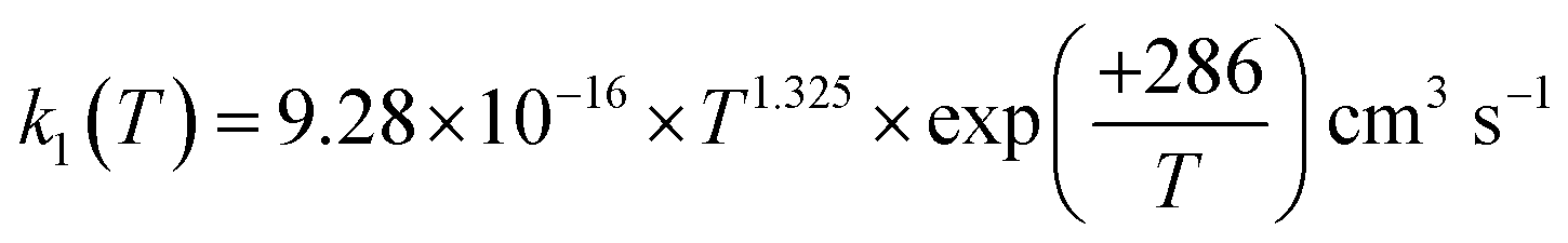
The rate coefficient for the reaction of hydrogen sulfide (H2S) with hydroxyl radicals (OH), which plays an important role in producing sulfuric acid and sulfates in the Earth's atmosphere, was computed by combining the high-accuracy coupled-cluster HEAT-345Q(P) method for energetics, W. H. Miller's semi-classical transition state theory (SCTST) and two-dimensional E,J-resolved master equation analysis (2DME) for kinetics. The title reaction proceeds by H-abstraction through a well-skipping mechanism directly yielding products H2O + SH. Tunneling effects are found to be important at the extremely low temperatures of the interstellar medium, but insignificant above 300 K. The rate coefficient k1(T, P), calculated over the temperature range T = 10–2500 K and a wide pressure range, is found to be effectively independent of pressure for T = 200–2500 K, in which range k1(T) can be represented by  . The results agree within 30% with the experimental data available in the T range of 230 to 550 K. For the range of 200–500 K of atmospheric interest, we recommend the rate coefficient expression:
  , based on the ab initio results of this work and the available experimental determinations.
Introduction
Hydrogen sulfide (H2S) emitted into the air originates from both natural and anthropogenic sources.1–11 In Earth's nature, H2S mainly stems from oceans and volcanic activities, while decomposition of organic wastes from animal farming and human activities also releases a significant amount of H2S.1–11 In the atmosphere, H2S is known to convert to sulfuric acid and sulfates, which cause acid rain and the formation of aerosols.1–11 In addition, hydrogen sulfide is a common component of natural gas and biomass.12 Hydrogen sulfide is a significant molecule found in the interstellar medium (ISM)13,14 and is often associated with sulfur-rich environments; it is one of the most primitive sulfur-bearing molecules detected in the ISM, appearing in various regions like cold dark clouds, diffuse clouds, and hot cores.13,14
The lifetime of H2S in the earth's atmosphere, principally controlled by its reaction with hydroxyl radicals (OH), is ca. 2.3 days using k1(298 K) = (5 ± 0.5) × 10−12 cm3 s−1 and 〈[OH]〉 = 106 cm−3.15,16
| | | H2S + OH(X2Π) → SH(X2Π) + H2O ΔHr(0 K) = −116.0 ± 0.4 kJ mol−1 | (1) |
Due to its important role in the atmosphere, reaction (1) has been studied extensively.1–11 Experimental rate coefficients have been determined for the temperature range of 230–550 K and found to be pressure-independent below 1 atm.1–11 Rate constant measurements at room temperature are scattered from 3.5 × 10⁻¹² to 5.5 × 10⁻¹² cm3 s−1,1–11 with a recommended k(298 K) of (5 ± 0.5) × 10−12 cm3 s−1.15,16 However, experimental k1(T) data are not available for T < 200 K as well as for T > 600 K, i.e. for interesting environments such as the ISM and combustion systems.
On the theoretical side,17–20 the reaction mechanism has been characterized in detail using CCSD(T)/aug-cc-pV(5+d)Z single-point energy calculations based on the CCSD(T)/aug-cc-pV(Q+d)Z geometry;17 however, this work does not report any kinetics analysis. Earlier, k1(T) rate constants were computed by direct dynamics (using a CVT/SCT approach) based on a potential energy surface constructed using the M06-2X/MG3S method.18 Quantum dynamics calculations based on a fitted potential energy surface using the UCCSD(T)-F12a/aug-cc-pVTZ level of theory have been recently reported;19 surprisingly, the calculated rate constants with these advanced techniques significantly differ from experimental values.19,20
In this work, the mechanism of the title reaction is characterized using the high-accuracy HEAT-345Q(P) method,21–23 which yields an accuracy of ca. ±0.5 kJ mol−1 for relative energies (i.e. reaction enthalpies and barriers) as compared to benchmark ATcT values in this case.24 The rate coefficient is computed over wide temperature and pressure ranges using a combination of W. H. Miller's semi-classical transition state theory (SCTST)25–29 and a two-dimensional E,J-resolved master equation approach.30–32 The calculated k1(T) values are compared with available experimental data. For the low-T and high-T regimes where there are no experimental results, this work provides high-level theoretical rate coefficients for kinetics modeling of ISM and combustion processes, among others.
Methodologies
High-accuracy coupled-cluster calculations
Under Cs symmetry, the reactants OH(X2Π) + H2S can correlate with the products SH(X2Π) + H2O on both 2A′ and 2A′′ electronic state potential energy surfaces (PES). All relevant stationary points on these PESs were optimized using the all-electron correlation coupled-cluster method including single, double, and non-iterative triple excitations (ae-CCSD(T))33–35 in conjunction with a basis set of cc-p(w)CVQZ36 (i.e. cc-pwCVQZ for the sulfur atom, cc-pCVQZ for the oxygen atom, and cc-pVQZ for hydrogen atoms). Total energies were then computed using the composite HEAT-345Q(P) method,21–23 which includes the contributions of different terms of energy:| | | EHEAT = ESCF,∞ + ΔECCSD(T),∞ + ΔET–(T),∞ +ΔEQ(P)–T + ΔEZPE + ΔEDBOC + ΔEscalar + ΔESO | (2) |
where ESCF,∞ is the SCF electronic energy extrapolated to the complete basis set limit (CBS) using aug-cc-p(w)CVXZ (where X = 3, 4, 5) basis sets; ΔECCSD(T),∞ is the electron correlation energy calculated using the CCSD(T) method and extrapolated to the CBS limit using the aug-cc-p(w)CVXZ (where X = 4, 5) basis set; ΔET–(T),∞ is the full triple excitation correction at the CBS limit; ΔEQ(P)–T is the Q(P) correction calculated as the difference between E[fc-CCSDTQ(P)/cc-pVDZ] and E[fc-CCSDT/cc-pVDZ]; ΔEDBOC is the diagonal Bohr–Oppenheimer correction; ΔEscalar is the scalar relativity effect; ΔESO is the spin–orbit correction, which includes electronic–rotational interactions, yielding −38.2 cm−1 for OH and −170.3 cm−1 for SH;37 ΔEZPE is the anharmonic zero-point vibrational energy, which is computed using second-order vibrational perturbation theory (VPT2).38 We used harmonic ZPEs calculated at the ae-CCSD(T)/aug-cc-p(w)CVQZ level of theory and anharmonic constants obtained from ae-CCSD(T)/aug-cc-p(w)CVTZ calculations to compute anharmonic ZPEs.
There is a hindered internal rotation (HIR) with a low vibrational frequency of 182 cm−1 in the H-abstraction transition structure (TS1, see Fig. 1), corresponding to the rotation of the H-atom of the HO group around the S−O axis. This HIR is assumed to be separable from the other vibrations, and it is independently treated as a 1D-HIR. A torsional PES was constructed using the ae-CCSD(T)/aug-cc-p(w)VQZ level of theory, and the 1D-Schrodinger equation was solved to obtain a vector of eigenvalues for this 1D-HIR using the LAMM code of the Multiwell software package (see Fig. S1 and S2 in the ESI‡).39 The resulting, directly counted torsional quantum states of the 1D-HIR were combined with the normal vibration states to obtain the overall quantum density and sum of “vibration” states for TS1.
 |
| | Fig. 1 Unscaled reaction energy profile of OH(X2Π) + H2S → H2O + SH(X2Π) constructed using the HEAT-345Q(P) method (see text). The benchmark ATcT value24 of the 0 K reaction enthalpy (in red) is included for comparison. | |
The CFOUR quantum chemical program was used for all CCSD(T) and CCSDT calculations.40 The CCSDTQ(P) calculations were carried out using the MRCC program,41 which is interfaced with CFOUR.
Two-dimensional E,J-resolved master equation calculations
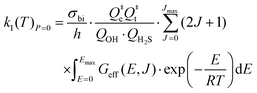
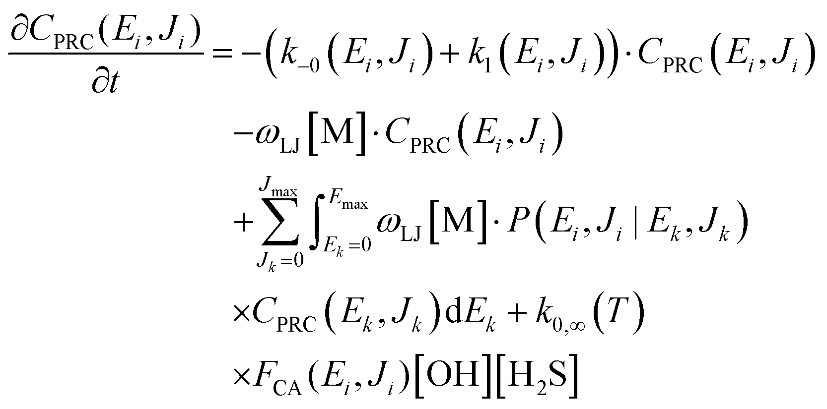
As shown in Fig. 1, the reaction of OH with H2S proceeds via a pre-reaction intermediate (PRC) before yielding products. The PRC, once formed in a specific E,J state through the variational entrance transition state TS0 (not shown in Fig. 1), can either re-dissociate back into the reactants through TS0, or react to form products through TS1, or lose/gain energy (E) and/or angular momentum (J) by collisions with the bath gas M. Therefore, the title reaction rate is, in principle, affected by pressure and a master equation needs to be solved to obtain rate constants, which depend on both temperature and pressure. The two-dimensional E,J-resolved master equation that describes the time evolution of the E,J-states of the PRC by its competing unimolecular reactions back to reactants and forward to products and by collisional E,J-transfer processes (see Fig. 1)—each with E,J-dependent rates—can be expressed as:30–32,42–46| |  | (3) |
where CPRC(Ei, Ji) is the population of the energized PRC† in a specific state, (Ei, Ji); ωLJ is the Lennard-Jones collisional rate (in cm3 molecule−1 s−1) and [M] (in molecules cm−3) is the concentration of the bath gas; P(Ei, Ji|Ek, Jk) is the transfer probability upon collision with M from an initial state, (Ek, Jk), to a final state, (Ei, Ji); k−0(Ei, Ji) is the microcanonical variational rate constant for the barrier-less re-dissociation of an energized PRC† back to initial reactants OH and H2S (see eqn (4)); k1(Ei, Ji) is the microcanonical rate constant for the H-abstraction step, computed using W. H. Miller's semi-classical transition state theory (SCTST)25–29,47,48 (see eqn (5)). It should be mentioned that multi-dimensional tunneling through the TS1 barrier is automatically accounted in the SCTST by the anharmonicity of the fully coupled vibration frequencies and the anharmonic ZPE. k0,∞(T) is the bimolecular rate constant for the capture of OH by H2S to form PRC† at the high-pressure limit (HPL) leading to 100% thermalized PRC (see eqn (6)) and FCA(Ei, Ji) is the nascent energy distribution of the formation of the resulting PRC† (see eqn (7)).
The variational transition state TS0 is characterized using variational RRKM theory49,50 (data provided in Table S1 in the ESI‡), i.e. the k−0(Ei, Ji) values for PRC re-dissociation are computed by minimizing the chemical flux through the dividing surface:
| |  | (4) |
| |  | (5) |
| |  | (6) |
| |  | (7) |
Here
h is Planck's constant.
σi is the reaction path degeneracy.
Q#e and
Q#t are the electronic and translational partition functions for TS0, respectively.
QOH is the complete partition function of the OH radical including electronic–rotation coupling interactions.
37QH2S is the complete partition function of H
2S.
Emax and
Jmax are the maximum internal energy and total angular momentum, respectively;
Emax = 70
![[thin space (1/6-em)]](https://www.rsc.org/images/entities/char_2009.gif)
000 cm
−1 and
Jmax = 300 were chosen to ensure that the calculated rate constants converge (better than 1%) for a wide temperature range of 10 K to 2500 K.
ρPRC(
E,
J) is the density of rovibrational states for PRC, while
G1(
E,
J) and
G0(
E,
J) are the sums of rovibrational states for TS1 and TS0 at the given (
E,
J), respectively. Vibrational
ρPRC(
Evib) and
GTS1(
Evib) are computed using the BDENS and SCTST codes of the Multiwell program.
39 Assuming that all stationary points are symmetric top, the rovibrational states can be computed using a
J-shifting approximation.
51,52| |  | (8) |
| |  | (9) |
| | | Erot(J, K) = 〈B〉·J·(J + 1) + (A − 〈B〉)·K2 with −J ≤ K ≤ +J | (10) |
All parameters including the energy bin, angular momentum bin, collisional parameters between PRC and the bath gas (air), and other data needed for the master equation simulations can be found in Table S2 (see the ESI
‡).
The rate coefficient k1(T, P) can be obtained by solving the master equation (eqn (3)) using two different (deterministic) methods, which necessarily yield the same result. In the first method, proposed by Barker,53 the yield of products YHS as opposed to that of the regenerated reactants (= 1 − YHS) is determined by solving eqn (3) without the source term, but starting from an initial energized PRC† population CPRC(E, J)(t = 0) taken equal to the nascent PRC formation distribution FCA(E, J) in eqn (7), which then evolves in time by re-dissociation to reactants and reaction to form the products HS + H2O in competition with the collisional energy transfer processes until the PRC population CPRC vanishes.37 The rate constant k1(T, P) follows from eqn (11):
| | | k1(T, P) =ϒSH × k0,∞(T), cm3 s−1 | (11) |
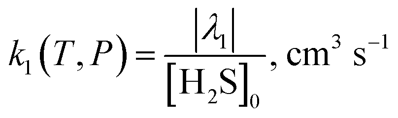
In the second method, suggested by Pilling,
54,55 the ME simulation is started with the initial reactants OH + H
2S, but with a very large excess concentration of H
2S (
i.e. [H
2S]
0 ≫ [OH]
0) to simplify the bimolecular reaction kinetics to a (pseudo)first-order decay of OH. The ME equation (
eqn (3)) is solved iteratively to find the lowest 1st eigenvalue (
λ1) using the ARPACK numerical software library.
56 The rate constant is obtained using
eqn (12):
| |  | (12) |
In this work, we used both methods, with identical results indeed.
57
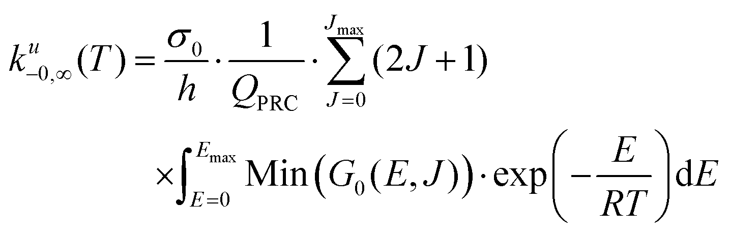
For the two extreme conditions of pressure approaching zero or infinity, the rate constants can be calculated using the analytical formulas given below. These analytical solutions, which are equivalent to the two-transition state (2-TS) kinetics model,58–60 were used to validate the numerical solutions of eqn (3).
For the zero-pressure limit (LPL):
| |  | (13a) |
with
| |  | (13b) |
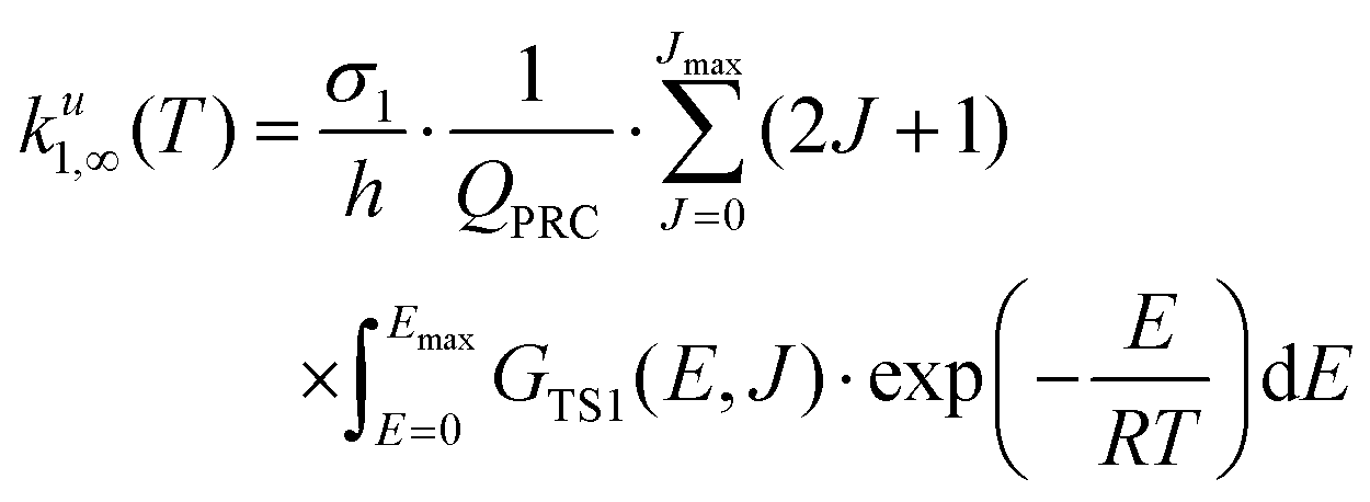
For the infinity-pressure limit (HPL):
| |  | (14a) |
in which
ku1,∞(
T) and
ku−0,∞(
T) are thermal rate coefficients in the high-pressure limit of the unimolecular reaction to products and re-dissociation of the PRC, respectively.
| |  | (14b) |
| |  | (14c) |
where
QPRC is the rotation–vibration partition function of PRC.
The pTS, pTDME, and fTDME codes of the Multiwell software package39 were used for the chemical kinetics analysis.
Results and discussion
Reaction mechanism
Key stationary points on the lowest-lying doublet electronic state potential energy surface (PES) displayed in Fig. 1 were characterized using a composite HEAT-345Q(P) method. As seen there, the capture of OH by H2S leads to the formation of a van der Waals complex (PRC), which has a binding energy of 6.6 kJ mol−1. PRC has a Cs symmetry with two (nearly degenerate) electronic states of 2A′′ and 2A′. When formed, PRC can re-dissociate back to the initial reactants via a loose, variational TS0 (not shown in Fig. 1) or can undergo a H-abstraction via a tight TS1 leading to a (highly vibrationally excited) pre-product complex (PPC†), which then decomposes quickly into products, H2O + SH. TS1 has no symmetry and lies 1.3 kJ mol−1 above the initial reactants. Given that overcoming (or tunneling through) TS1 is the rate determining step, it is important to understand the contributions of the various terms to the energy barrier in the HEAT calculations. As shown in Table 1, the SCF energy is the most important, and it significantly overpredicts the effective barrier (i.e. relative to the reactants) at +59.9 kJ mol−1. The CCSD(T) electron correlation is the second most important, and it brings the barrier down to +0.6 kJ mol−1. The ZPE correction is the third most important, and it increases the barrier again by 2.6 kJ mol−1. It should be mentioned that the 1D-HIR treatment increases the barrier by +0.36 kJ mol−1 due to the change of ZPE. The higher-level corrections (HLC) that go beyond the CCSD(T) lower the barrier by −1.9 kJ mol−1. Finally, the scalar relativity effects and spin–orbit correction also have important contributions, but they have opposite signs.
Table 1 Individual contributions (kJ mol−1) of the various terms to the relative energy of TS1, the PRC and the reaction enthalpy at 0 K using the HEAT-345Q(P) method
| Term |
TS1 |
PRC |
H2O + SH |
|
Heats of formation at 0 K of OH (37.278 ± 0.022 kJ mol−1), H2S (−17.36 ± 0.18 kJ mol−1), H2O (−238.903 ± 0.022 kJ mol−1), and SH (142.81 ± 0.18 kJ mol−1) are taken from ATcT (ref. 24).
|
| δESCF→∞ |
59.91 |
−6.64 |
−78.81 |
| δECCSD(T)→∞ |
−59.32 |
−6.74 |
−45.30 |
| δECCSDT→∞ |
−1.32 |
0.01 |
0.37 |
| δECCSDTQ(P) |
−0.58 |
−0.04 |
−0.40 |
| δEscalar |
−0.35 |
−0.16 |
−0.59 |
| δEZPE |
2.54 |
6.38 |
9.93 |
| δEDBOC |
−0.04 |
0.18 |
−0.28 |
| δEspin–orbit |
0.46 |
0.46 |
−1.58 |
| HEAT |
1.30 |
−6.55 |
−116.66 ± 0.5 |
| ATcT |
|
|
−116.0 ± 0.4a |
The title reaction was theoretically studied earlier.17–20 A comparison of relative energies obtained in this work with other values reported in the literature is summarized in Table 2. As seen there, the agreement between different levels of theory is good, i.e. within 3 kJ mol−1. It should be noted that the energies reported in the literature17–20 do not include the higher-level corrections (such as CCSDT and CCSDTQ(P)) as well as other corrections (anharmonic correction, spin–orbit, and scalar relativity effects). As compared to the benchmark ATcT value24 for the reaction enthalpy, the HEAT-345Q(P) value is in excellent agreement, within 0.66 kJ mol−1. To the best of our knowledge, the HEAT-345Q(P) method used in this work is the highest level of theory that has been applied to the title reaction. Surprisingly, the DFT calculations with the M06-2X/MG3S method18 yield an effective barrier of 1.05 kJ mol−1, which is only 0.25 kJ mol−1 lower than the HEAT-345Q(P) value.
Table 2 A comparison of energiesa (kJ mol−1) relative to initial reactants (OH + H2S) calculated using the HEAT-345Q(P) method with values reported in the literature
| Method |
TS1 |
H2O + SH |
PRC |
|
The values given in parentheses are exclusive of ZPE correction.
Taken from ref. 17. It was calculated using the fc-CCSD(T)/aug-cc-pV(5+d)Z//fc-CCSD(T)/aug-cc-pV(Q+d)Z level of theory.
Reported in ref. 18.
From ref. 19.
Taken from the benchmark ATcT (ref. 24).
|
| HEAT-345Q(P) |
1.30 (−1.24) |
−116.66 ± 0.5 (−126.59) |
−6.55 (−12.93) |
| CCSD(T)/aV(5+d)Zb |
3.14 (0.46) |
−113.22 (−123.47) |
−6.03 (−13.81) |
| MCG3/3//MC-QCISD/3c |
(1.72) |
(−131.38) |
N/A |
| M06-2X/MG3Sc |
1.05 (−1.00) |
(−123.43) |
N/A |
| UCCSD(T)-F12a/aVTZd |
2.37 (−0.43) |
−113.70 (−124.20) |
−7.72 (−14.00) |
| ATcTe |
N/A |
−116.0 ± 0.4 |
N/A |
Reaction rate coefficients
The experimental k1 results (at T = 230–550 K) are not indicative of pressure dependence for P < 1 atm.1–11 To check the possible effects of pressure on the rate coefficient, we computed the ratio of rate constants at the HPL using eqn (14) and rate constants at the LPL using eqn (13). The results presented in Fig. 2 show that the rate constant is effectively independent of pressure for T ≥ 200 K, i.e. for example, for all applications relevant to atmospheric and combustion environments. The pressure dependence becomes noticeable when T < 100 K, and it increases sharply when temperature decreases, for example, to temperatures as in the ISM. However, as the pressure in the ISM is extremely low, the title reaction is beyond doubt in the LPL in this environment. There are three different (combined) causes for the lack of pressure dependence of the rate constant at T > 200 K: (i) first, the van der Waals complex PRC lies in a shallow well of only 6.6 kJ mol−1, so its collisional stabilization and thermalization is unlikely to compete effectively with its prompt re-dissociation except at extremely high pressures; (ii) the barrier is very low, only 1.3 kJ mol−1 above the initial reactants, such that tunneling through the barrier is expected to be a minor effect except at very low temperatures; and (iii) the imaginary vibration frequency along the reaction coordinate of TS1, which is inversely proportional to the width of the barrier, has a moderate value of only 882i cm−1. These three factors combined keep tunneling effects minor for T > 300 K (see Fig. 3). As shown in Fig. 3, the tunneling factor increases sharply once T < 100 K. It may be noted that quantum mechanical tunneling is the main cause for the pressure-dependent rate of the similar reaction of OH and HNO3 as shown in a previous study.61 Note that the results of fall-off curves (i.e. k(T, P)) at very low temperatures are provided in the ESI‡ (see Fig. S3, ESI‡).
 |
| | Fig. 2 Ratio of the calculated k1,P=∞(T)/k1,P=0(T) of the H2S + OH reaction as a function of temperature. The rate coefficient is effectively independent of pressure for T > 200 K. | |
 |
| | Fig. 3 Tunneling factor of the H2S + OH reaction from first principles as a function of temperature. | |
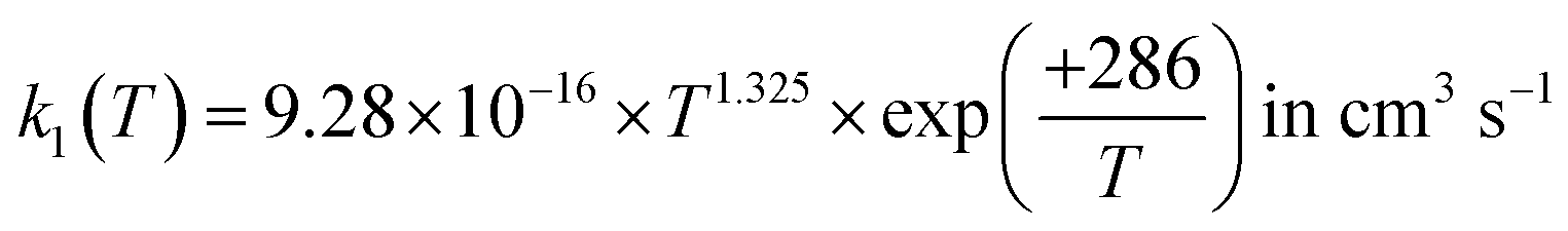
For the following discussion, the results of this work for k1(T, P = 0) were computed at the LPL, using eqn (13a) and (13b), and denoted as k1(T, 0). Fig. 4 shows a comparison of our theoretical LPL results with various experimental data for T = 230–550 K. In general, the agreement between theory and experiment is good (within ca. 30%). Our ab initio k1(T, 0) data (solid black curve) are in line with the higher experimental values, while when increasing the barrier of TS1 by 0.5 kJ mol−1 (the possible energy error of the HEAT-345Q(P) method), the calculated data (dotted pink curve) agree well with the lower experimental values. Fig. 5 shows a fit of a modified Arrhenius equation to the combined set of our theoretical LPL results and all experimental data in Fig. 4: 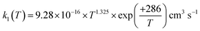 for T = 200–500 K, with equal weights given to our ab initio data and the combined experimental data; this fit is represented by the solid red line in Fig. 5. The k1(T) fit equation above is recommended by this work for atmospheric applications. Two earlier recommendations15,16 are also shown in Fig. 5; as can be seen, they differ from our present recommendation either at the higher or at the lower temperatures of this range.
 |
| | Fig. 4 A comparison of the calculated LPL rate coefficients k1(T, P = 0) from this work with experimental data (symbols)1–11 and two k1(T) expressions recommended in the literature15,16 for the temperature range of 200–550 K. The solid black curve represents our k1(T, P = 0) data from first principles, while the dotted pink curve is obtained by raising the TS1 barrier by +0.5 kJ mol−1 (to 1.8 kJ mol−1), which is the expected possible error of the HEAT-345Q(P) method for this reaction system (see text). | |
 |
| | Fig. 5 A comparison of the rate coefficient recommended in this work (solid red curve; see text)  for T = 200–500 K with the experimental data (symbols)1–11 as well as two other recommendations15,16 in the literature. for T = 200–500 K with the experimental data (symbols)1–11 as well as two other recommendations15,16 in the literature. | |
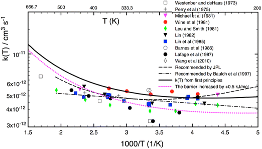
Fig. 6 shows LPL rate coefficients calculated for the extensive temperature range from 10 to 2500 K. The theoretical curves (the ab initio result and that for TS1 0.5 kJ mol−1 higher) have a pronounced concave shape. Starting from a temperature of 10 K, with k1(10 K, P = 0) close to 10−10 cm3 s−1, the rate coefficient decreases as the temperature increases, to reach a minimum at about 250 K, and then increases again with temperature. Interestingly, at 10 K—characteristic of the ISM environment—k1(P = 0) is about 20 times higher than at room temperature (5 × 10⁻¹² cm3 s−1), mainly due to quantum tunneling effects. For the T range 200–2500 K, our ab initio LPL results can be represented in good approximation by the modified Arrhenius expression:  .
.
 |
| | Fig. 6 Rate constants calculated using SCTST/2DME/HEAT approaches (this work) for a wide temperature range of 10–2500 K. The solid curve represents values from first principles. The dotted curve represents values obtained by raising the TS1 barrier by +0.5 kJ mol−1. Experimental data (symbols)1–11 are also included for comparison. | |
Computed rate coefficient data k1(T) were reported earlier by Ellingson et al.18 using the CVT/SCT method based on a PES constructed using the M06-2X/MG3S DFT-method. In Table 3, the CVT/SCT-based values are compared with our SCTST/2DME k1(T), showing good agreement, within ca. 30%, over a wide temperature range of 200 to 2400 K. One can expect such a good agreement because the M06-2X barrier of TS1 agrees very well with the HEAT method's value (see Table 2); however, this agreement may be due to a cancellation of errors in the DFT method.
Table 3 A comparison of rate constants calculated using the SCTST/2DME approach in this work with those obtained using the CVT/SCT method and Polyrate software
|
T (K) |
SCTST/2DME (ab initio)a |
SCTST/2DME (adjusted barrier)b |
CVT/SCTc |
Differenced (%) |
This work, k1(T, P = 0) calculated from first principles (see text).
This work, with the energy of TS1 increased by +0.5 kJ mol−1 (see text).
Taken from ref. 18 based on a PES constructed using the M06-2X/MG3S level of theory.
The difference is defined as  . .
|
| 200 |
4.94 × 10⁻¹² |
3.78 × 10⁻¹² |
4.38 × 10⁻¹² |
−16 |
| 250 |
4.84 × 10⁻¹² |
3.87 × 10⁻¹² |
4.20 × 10⁻¹² |
−9 |
| 300 |
5.08 × 10⁻¹² |
4.20 × 10⁻¹² |
4.23 × 10⁻¹² |
−1 |
| 350 |
5.53 × 10⁻¹² |
4.70 × 10⁻¹² |
4.50 × 10⁻¹² |
4 |
| 400 |
6.15 × 10⁻¹² |
5.33 × 10⁻¹² |
4.87 × 10⁻¹² |
9 |
| 600 |
1.00 × 10⁻¹¹ |
9.12 × 10⁻¹² |
7.25 × 10⁻¹² |
21 |
| 1000 |
2.24 × 10⁻¹¹ |
2.12 × 10⁻¹¹ |
1.57 × 10⁻¹¹ |
26 |
| 1500 |
3.89 × 10⁻¹¹ |
3.76 × 10⁻¹¹ |
2.61 × 10⁻¹¹ |
31 |
| 2400 |
5.57 × 10⁻¹¹ |
5.45 × 10⁻¹¹ |
6.66 × 10⁻¹¹ |
−22 |
Conclusions
In this work, high-level theoretical calculations were used to readdress the reaction mechanism and kinetics of the H2S + OH reaction: the high-accuracy HEAT method for energetics and a two-dimensional E,J-resolved master equation analysis for the kinetics. The reaction is shown to proceed by hydrogen abstraction via a well-skipping mechanism,62 leading to the formation of H2O and SH. The calculated reaction enthalpy is in excellent agreement with the benchmark ATcT value. The rate coefficient was calculated from first principles over wide temperature (10–2500 K) and pressure ranges. Pressure dependence was found to be limited to the T range below 200 K, where it becomes gradually very important as T decreases. The rate coefficient data agree well with the available experimental data at 200–500 K, within ca. 30%, which is similar to the spread of the different measurements. For the range T = 200–500 K, we recommend the rate expression  for atmospheric applications. For applications in the ISM environment and in combustion processes, i.e. for temperatures where experimental data are not available, we provide high-level theoretical results.
Conflicts of interest
There are no conflicts of interest to declare.
Data availability
The data that support the findings of this study are available within the article and its ESI.‡ Detailed theoretical data that support the findings of this study are available from the corresponding author upon reasonable request.
Acknowledgements
This work was done by TLN and JFS (the University of Florida) through support from the U.S. Department of Energy, Office of Basic Energy Sciences under Award DE-SC0018164. TLN would like to thank the Department of Chemistry, the University of Florida for the financial support.
References
- A. A. Westenberg and N. Dehaas, J. Chem. Phys., 1973, 59, 6685–6686 CrossRef
 .
.
- R. A. Perry, R. Atkinson and J. N. Pitts, J. Chem. Phys., 1976, 64, 3237–3239 CrossRef .
- R. A. Cox and D. Sheppard, Nature, 1980, 284, 330–331 CrossRef .
- P. H. Wine, N. M. Kreutter, C. A. Gump and A. R. Ravishankara, J. Phys. Chem., 1981, 85, 2660–2665 CrossRef .
- M. T. Leu and R. H. Smith, J. Phys. Chem., 1982, 86, 73–81 CrossRef CAS .
- J. V. Michael, D. F. Nava, W. D. Brobst, R. P. Borkowski and L. J. Stief, J. Phys. Chem., 1982, 86, 81–84 CrossRef CAS .
- C. L. Lin, Int. J. Chem. Kinet., 1982, 14, 593–598 CrossRef .
- I. Barnes, V. Bastian, K. H. Becker, E. H. Fink and W. Nelsen, J. Atmos. Chem., 1986, 4, 445–466 CrossRef .
- C. Lafage, J. F. Pauwels, M. Carlier and P. Devolder, J. Chem. Soc., Faraday Trans. 2, 1987, 83, 731–739 RSC .
- H. T. Wang, D. S. Zhu, W. P. Wang and Y. J. Mu, Chin. Sci. Bull., 2010, 55, 2951–2955 CrossRef .
- Y. L. Lin, N. S. Wang and Y. P. Lee, Int. J. Chem. Kinet., 1985, 17, 1201–1214 CrossRef .
- A. Pudi, M. Rezaei, V. Signorini, M. P. Andersson, M. G. Baschetti and S. S. Mansouri, Sep. Purif. Technol., 2022, 298, 121448 CrossRef .
- P. Thaddeus, R. W. Wilson, M. L. Kutner, K. B. Jefferts and A. A. Penzias, Astrophys. J., 1972, 176, L73–L76 CrossRef .
- Y. C. Minh, W. M. Irvine and L. M. Ziurys, Astrophys. J., 1989, 345, L63–L66 CrossRef PubMed .
- D. L. Baulch, C. T. Bowman, C. J. Cobos, R. A. Cox, T. Just, J. A. Kerr, M. J. Pilling, D. Stocker, J. Troe, W. Tsang, R. W. Walker and J. Warnatz, J. Phys. Chem. Ref. Data, 2005, 34, 757–1397 CrossRef .
-
J. B. Burkholder, S. P. Sander, J. P. D. Abbatt, J. R. Barkeri, C. Cappa, J. D. Crounse, T. S. Dibble, R. E. Huie, C. E. Kolbi, M. J. Kurylo, V. L. Orkin, C. J. Percival, D. M. Wilmouth and P. H. Wine, Chemical Kinetics and Photochemical Data for Use in Atmospheric Studies, Evaluation No. 19, JPL Publication 19-5, Jet Propulsion Laboratory, Pasadena, 2019, http://jpldataeval.jpl.nasa.gov.
- M. Tang, X. R. Chen, Z. Sun, Y. M. Xie and H. F. Schaefer, J. Phys. Chem. A, 2017, 121, 9136–9145 CrossRef PubMed .
- B. A. Ellingson and D. G. Truhlar, J. Am. Chem. Soc., 2007, 129, 12765–12771 CrossRef PubMed .
- L. L. Ping, Y. F. Zhu, A. Y. Li, H. W. Song, Y. Li and M. H. Yang, Phys. Chem. Chem. Phys., 2018, 20, 26315–26324 RSC .
- H. P. Xiang, Y. P. Lu, H. W. Song and M. H. Yang, Chin. J. Chem. Phys., 2022, 35, 200–206 CrossRef .
- A. Tajti, P. G. Szalay, A. G. Csaszar, M. Kallay, J. Gauss, E. F. Valeev, B. A. Flowers, J. Vazquez and J. F. Stanton, J. Chem. Phys., 2004, 121, 11599–11613 CrossRef .
- Y. J. Bomble, J. Vazquez, M. Kallay, C. Michauk, P. G. Szalay, A. G. Csaszar, J. Gauss and J. F. Stanton, J. Chem. Phys., 2006, 125, 064108 CrossRef PubMed .
- M. E. Harding, J. Vazquez, B. Ruscic, A. K. Wilson, J. Gauss and J. F. Stanton, J. Chem. Phys., 2008, 128, 111102 CrossRef PubMed .
-
B. Ruscic and D. H. Bross, Active Thermochemical Tables (ATcT) values based on ver. 1.202 of the Thermochemical Network, 2025 Search PubMed .
- W. H. Miller, Faraday Discuss., 1977, 62, 40–46 RSC .
- W. H. Miller, R. Hernandez, N. C. Handy, D. Jayatilaka and A. Willetts, Chem. Phys. Lett., 1990, 172, 62–68 Search PubMed .
- W. H. Miller, R. Hernandez, C. B. Moore and W. F. Polik, J. Chem. Phys., 1990, 93, 5657–5666 CrossRef .
- M. J. Cohen, N. C. Handy, R. Hernandez and W. H. Miller, Chem. Phys. Lett., 1992, 192, 407–416 Search PubMed .
- R. Hernandez and W. H. Miller, Chem. Phys. Lett., 1993, 214, 129–136 CrossRef .
- T. L. Nguyen and J. F. Stanton, J. Phys. Chem. A, 2015, 119, 7627–7636 Search PubMed .
- T. L. Nguyen and J. F. Stanton, J. Phys. Chem. A, 2018, 122, 7757–7767 CrossRef PubMed .
- T. L. Nguyen and J. F. Stanton, J. Phys. Chem. A, 2020, 124, 2907–2918 CrossRef PubMed .
- J. F. Stanton, Chem. Phys. Lett., 1997, 281, 130–134 CrossRef .
- K. Raghavachari, G. W. Trucks, J. A. Pople and M. Headgordon, Chem. Phys. Lett., 1989, 157, 479–483 CrossRef .
- R. J. Bartlett, J. D. Watts, S. A. Kucharski and J. Noga, Chem. Phys. Lett., 1990, 165, 513–522 CrossRef .
- T. H. Dunning, J. Chem. Phys., 1989, 90, 1007–1023 CrossRef .
- T. L. Nguyen, B. Ruscic and J. F. Stanton, J. Chem. Phys., 2019, 150, 084105 CrossRef PubMed .
-
I. M. Mills, Vibration-Rotation Structure in Asymmetric- and Symmetric-Top Molecules, in Molecular Spectroscopy: Modern Research, ed. K. N. Rao and C. W. Mathews, Academic Press, New York, 1972, vol. 1, p. 115 Search PubMed .
-
J. R. Barker, T. L. Nguyen, J. F. Stanton, C. Aieta, M. Ceotto, F. Gabas, T. J. D. Kumar, C. G. L. Li, L. L. Lohr, A. Maranzana, N. F. Ortiz, J. M. Preses, J. M. Simmie, J. A. Sonk and P. J. Stimac, MULTIWELL, Program Suite Climate and Space Sciences and Engineering, University of Michigan, Ann Arbor, MI 48109-2143, 2024.
- D. A. Matthews, L. Cheng, M. E. Harding, F. Lipparini, S. Stopkowicz, T. C. Jagau, P. G. Szalay, J. Gauss and J. F. Stanton, J. Chem. Phys., 2020, 152, 214108 CrossRef PubMed .
- M. E. A. Kalley, J. Chem. Phys., 2013, 139, 094105 CrossRef .
- S. H. Robertson, M. J. Pilling, K. E. Gates and S. C. Smith, J. Comput. Chem., 1997, 18, 1004–1010 Search PubMed .
- S. J. Jeffery, K. E. Gates and S. C. Smith, J. Phys. Chem., 1996, 100, 7090–7096 CrossRef .
- A. W. Jasper, K. M. Pelzer, J. A. Miller, E. Kamarchik, L. B. Harding and S. J. Klippenstein, Science, 2014, 346, 1212–1215 CrossRef .
- J. A. Miller, S. J. Klippenstein and C. Raffy, J. Phys. Chem., 2002, 106, 4904–4913 CrossRef .
- P. K. Venkatesh, A. M. Dean, M. H. Cohen and R. W. Carr, J. Chem. Phys., 1999, 111, 8313–8329 CrossRef .
- T. L. Nguyen, J. F. Stanton and J. R. Barker, Chem. Phys. Lett., 2010, 499, 9–15 CrossRef CAS .
- T. L. Nguyen, J. F. Stanton and J. R. Barker, J. Phys. Chem. A, 2011, 115, 5118–5126 CrossRef CAS PubMed .
- W. L. Hase, Acc. Chem. Res., 1983, 16, 258–264 CrossRef CAS .
- D. G. Truhlar, B. C. Garrett and S. J. Klippenstein, J. Phys. Chem., 1996, 100, 12771–12800 CrossRef CAS .
- J. M. Bowman, J. Phys. Chem., 1991, 95, 4960–4968 CrossRef CAS .
- W. H. Miller, J. Am. Chem. Soc., 1979, 101, 6810–6814 CrossRef .
- J. R. Barker, Int. J. Chem. Kinet., 2001, 33, 232–245 CrossRef .
- M. A. Hanninglee, N. J. B. Green, M. J. Pilling and S. H. Robertson, J. Phys. Chem., 1993, 97, 860–870 CrossRef .
-
S. H. Robertson, D. R. Glowacki, C. Morley, C. H. Liang, R. J. Shannon, M. Blitz, P. Seakins, M. J. Pilling and J. N. Harvey, MESMER (Master Equation Solver for Multi Energy-well Reactions): An open source, general purpose program for calculating rate coefficients through solving the chemical master equation, University of Leeds, 2018.
-
B. Lehoucq, D. C. Sorensen and C. Yang, Society for Industrial and Applied Mathematics. ARPACK users' guide solution of large-scale eigenvalue problems with implicitly restarted Arnoldi methods, Philadelphia, PA., 1998, 1 electronic text (xv), p. 142.
- T. L. Nguyen, D. H. Bross, B. Ruscic, G. B. Ellison and J. F. Stanton, Faraday Discuss., 2022, 238, 405–430 Search PubMed .
- T. L. Nguyen and J. Peeters, Phys. Chem. Chem. Phys., 2021, 23, 16142–16149 RSC .
- E. E. Greenwald, S. W. North, Y. Georgievskii and S. J. Klippenstein, J. Phys. Chem. A, 2005, 109, 6031–6044 CrossRef PubMed .
- W. H. Miller, J. Chem. Phys., 1976, 65, 2216–2223 CrossRef CAS .
- T. L. Nguyen and J. F. Stanton, J. Phys. Chem. Lett., 2020, 11, 3712–3717 CrossRef CAS .
- N. J. Labbe, R. Sivaramakrishnan and S. J. Klippenstein, Proc. Combust. Inst., 2015, 35, 447–455 CrossRef .
Footnotes |
| † In loving memory of Prof. John F. Stanton (1961–2025). |
| ‡ Electronic supplementary information (ESI) available: Optimized geometries, rovibrational parameters, anharmonic constants, calculated rate coefficients, and additional figures. See DOI: https://doi.org/10.1039/d5cp01904d |
|
| This journal is © the Owner Societies 2025 |
Click here to see how this site uses Cookies. View our privacy policy here. 
 Open Access Article
 This Open Access Article is licensed under a Creative Commons Attribution-Non Commercial 3.0 Unported Licence
 *a,
Jozef
Peeters
*a,
Jozef
Peeters
 . The results agree within 30% with the experimental data available in the T range of 230 to 550 K. For the range of 200–500 K of atmospheric interest, we recommend the rate coefficient expression:
  , based on the ab initio results of this work and the available experimental determinations.


 for T = 200–500 K, with equal weights given to our ab initio data and the combined experimental data; this fit is represented by the solid red line in Fig. 5. The k1(T) fit equation above is recommended by this work for atmospheric applications. Two earlier recommendations15,16 are also shown in Fig. 5; as can be seen, they differ from our present recommendation either at the higher or at the lower temperatures of this range.

 for T = 200–500 K with the experimental data (symbols)1–11 as well as two other recommendations15,16 in the literature.
 .
.
 .
.
 for atmospheric applications. For applications in the ISM environment and in combustion processes, i.e. for temperatures where experimental data are not available, we provide high-level theoretical results.