
 Open Access Article
 This Open Access Article is licensed under a
 Creative Commons Attribution 3.0 Unported Licence
BSE@GW-based protocol for spin-vibronic quantum dynamics using the linear vibronic coupling model. Formulation and application to an Fe(II) compound†
Florian
Bogdain
a,
Sebastian
Mai
 b,
Leticia
González
bc and
Oliver
Kühn
*a
b,
Leticia
González
bc and
Oliver
Kühn
*a
aInstitute of Physics, University of Rostock, Albert-Einstein-Str. 23-24, 18059 Rostock, Germany. E-mail: oliver.kuehn@uni-rostock.de
bInstitute of Theoretical Chemistry, Faculty of Chemistry, University of Vienna, Währinger Straße 17, 1090 Vienna, Austria
cVienna Research Platform on Accelerating Photoreaction Discovery, University of Vienna, Währinger Straße 17, 1090 Vienna, Austria
First published on 2nd July 2025
Abstract
A protocol for generating potential energy surfaces and performing photoinduced nonadiabatic multidimensional wave packet propagation is presented. The workflow starts with the parameterization of a linear vibronic coupling (LVC) Hamiltonian using the Green's function – Bethe–Salpeter equation (BSE@GW) approach. In a second step, the LVC model is used as input for multi-layer multi-configurational time-dependent Hartree (ML-MCTDH) wave packet propagation. To facilitate automated ML tree generation, a spectral clustering algorithm is applied based on a correlation matrix obtained from nuclear coordinate expectation values of a full-dimensional time-dependent Hartree (TDH) simulation. The performance of the protocol is tested on the photoinduced spin-vibronic dynamics of a transition metal complex, [Fe(cpmp)]2+. For this example, it is shown that BSE@GW provides a more robust description of the character of the transitions contributing to the absorption spectrum compared to TD-DFT. Furthermore, the LVC parameterization is tested against explicit calculations of potential energy curves to find the validity of the linear approximation over a wide range of normal mode elongation. Finally, the flexibility of spectral clustering is used to generate different ML trees, resulting in very different numerical efficiencies for ML-MCTDH propagation. In terms of electronic structure and dimensionality, [Fe(cpmp)]2+ is a challenging example, suggesting that the new protocol should be applicable to a wide range of systems.
1 Introduction
Photoexcited spin-vibronic dynamics is the consequence of the interplay between nonadiabatic and spin–orbit couplings (SOCs) comprising several regimes, depending on the relative magnitudes of these couplings.1 It is of particular relevance for systems containing transition metals where large SOC comes together with the metal's electronic structure and ligand effects giving rise to a large density of valence excited states. Due to their relevance for various practical applications, in particular first-row transition metals are a prime target of current research.2–6Electronic excitations in transition metal complexes can be classified as being of metal/ligand centered (MC/LC) or charge transfer type, e.g. metal-to-ligand charge transfer (MLCT) or vice versa (LMCT). Stepping from rather successful 4d/5d to 3d transition metals leads to a drastically altered electronic structure as far as the interplay between these types of transitions is concerned. This often comes along with a much reduced MLCT lifetime, which is disadvantageous, e.g. for catalytic applications.7 This is a challenge for ligand design and in particular systems with carbene ligands showed MLCT lifetimes in the nanosecond regime have been reported.8
The challenge to theory provided by transition metal compounds with typical organic ligands is twofold. First, the electronic structure is notorious for the many complications arising from static and dynamic correlations. Second, dynamics simulations for typical systems will have to cope with hundreds of nuclear degrees of freedom (DOFs). In terms of electronic structure theory, density functional theory (DFT) with tailored exchange–correlation (XC) functionals has proven a low-cost yet reasonably accurate alternative to expensive wave function calculations.9 In particular non-empirically tuned range-separated functionals10,11 perform rather well, although often the actual agreement, e.g. with absorption spectra is hard to predict clear beforehand.12 A particular challenge is provided by the interplay between MC and MLCT transition as shown in ref. 13. Absorption spectra at the Franck–Condon geometry are often the target when it comes to the assessment of electronic structure methods. However, as also demonstrated in ref. 13 using trajectory surface hopping (TSH)14 different parameterizations of a range-separated functional can lead to rather different photodynamics even though the absorption spectra are similar.
A viable alternative to common time-dependent density functional theory (TD-DFT) calculations is the Green's function, Bethe–Salpeter equation (BSE@GW) approach.15–18 It has demonstrated notably strong performance for solids19–21 and interfaces,22 but also delivered accurate results for single-point calculations across a wide range of molecular systems.23–26 Recently, we have provided a systematic investigation of electronic excitations of first-row transition metal compounds using BSE@GW.27 It was shown that BSE@GW often outperforms TD-DFT in terms of the prediction of absorption spectra. Even more important, however, is the observation that the mixing of MLCT and MC states can be accounted for with results being robust against variations of the XC functional.
In the context of dynamics simulations, a rather successful approximation to the PES is the linear vibronic coupling (LVC) model,1,28,29 which builds on the availability of gradients on the PES. While being standard for TD-DFT, computations of gradients at the BSE@GW level of theory remain scarce and are restricted to the numerical determination.30 Furthermore, to our knowledge there exists no straightforward and easy-to-use implementation of numerical gradients at the BSE@GW level of theory. This work aims at filling this gap, yielding a LVC model that paves the way to perform TSH31 or full quantum mechanical dynamics simulations in the form of MCTDH.32–34
The multi-configuration time-dependent Hartree (MCTDH) method has proven a versatile approach to high-dimensional quantum dynamics. Introduced in 1990 by Meyer and coworkers35,36 there have been numerous applications, e.g., to nonadiabatic electron-vibrational dynamics,37 including transition metal compounds,1,38,39 excitation energy transfer in pigment-protein complexes,40,41 but also to vibrational dynamics42,43 (for an overview, see also ref. 44). It should be noted that for efficiency MCTDH requires to have at hand a Hamiltonian in the form of a sum of products. Therefore, the LVC model discussed above is ideally suited for the combination with MCTDH dynamics. A boost concerning the dimensionality came with the multi-layer extension (ML-MCTDH) introduced by Wang and Thoss45 and later generalized in ref. 46 and 47. While in MCTDH the wave packets are expanded into Hartree products of single-particle functions (SPFs), in ML-MCTDH the idea is to combine strongly correlated DOFs into multidimensional particles, which in turn are expanded in MCTDH form. This is repeated until one- or low-dimensional particles are obtained. The resulting wave packet has a tree-like (ML-tree) structure that needs to be converged with respect to the number of SPFs assigned to the branches. This results in the challenge to find cost-efficient ML-trees, since the numerical performance in terms of CPU time can vary vastly for different trees.48 While there are simple guidelines for combining modes (e.g. similar frequencies), standardized routines for the systematic generation of reliable ML-tree structures remain scarce. Recently, Mendive-Tapia et al. proposed to use hierarchical clustering for generating ML-trees, focusing on vibrational dynamics.49 In this work we will present a method based on spectral clustering,50 yielding ML-trees for nonadiabatic electron-vibrational dynamics.
The computational workflow presented in this paper starts with the determination of a full-dimensional LVC coupling Hamiltonian using BSE@GW (Section 2.2) that serves as an input for the generation of ML-trees using spectral clustering (Section 2.3). The new protocol will be applied to the [Fe(cpmp)]2+ complex (cpmp = 6,2′-′carboxypyridyl-2,2′-methylamine-pyridyl-pyridin) shown in Fig. 1. The design of this pseudo-octahedral complex follows two strategies for obtaining long-lived MLCT states, i.e. forming a close to octahedral coordination sphere such as to maximize the ligand field splitting and destabilizing the MC states by electron-rich ligands while simultaneously stabilizing the MLCT states by π-acceptor groups.51
 | ||
| Fig. 1 Chemical structure and geometry of the [Fe(cpmp)]2+ complex investigated in this work (for synthesis and experimental characterization, see ref. 51). | ||
Previous research has studied the excited state dynamics of this system using both classical TSH13 and ML-MCTDH52 dynamics simulations. In both cases, TD-DFT was the underlying level of theory at which the PES was calculated. The range-separated LC-BLYP(α, ω) functional was used, where the parameters α and ω were tuned non-empirically. The results presented in Section 4 primarily serve to illustrate the new protocol rather than introduce novel insights into the photophysics of this particular complex. However, this paper includes a valuable comparison of the absorption spectrum assignments for TD-DFT and BSE@GW, along with a detailed investigation of the validity of the LVC model.
2 Theoretical methods
2.1 BSE@GW theory
Within the BSE@GW approach, optical transitions are obtained by solving the following eigenvalue problem53,54 | (1) |
The matrix elements are given by55
 | (2) |
 | (3) |
2.2 Linear vibronic coupling model
The molecular Hamiltonian in diabatic representation reads as follows29,60 | (4) |
 | (5) |
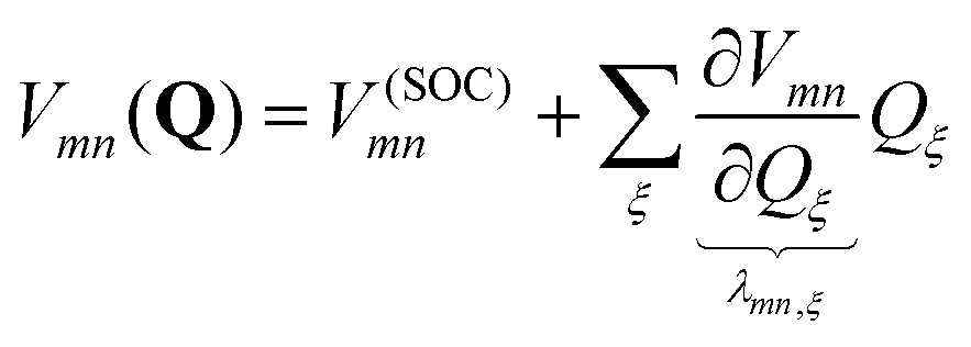 | (6) |
 | (7) |
 | (8) |
 at different geometries R and R′ can be constructed in a three-step process,66 starting with the computation of the overlap of the atomic orbitals |χμ〉. This step is widely used in quantum chemistry computations and code is readily available. Afterward, these overlaps can be combined with the molecular orbitals coefficients to obtain the overlap between different molecular orbitals.
 | (9) |
 of Slater determinants |Φl〉 = |ϕl(1),…,ϕl(nα+nβ)|, which are then combined with their corresponding configuration interaction (CI) coefficients dIk to produce the overlap between different adiabatic electronic states.
 | (10) |
This LVC Hamiltonian may also be extended by an additional term, accounting for the interaction with an external electric field, ![[E with combining right harpoon above (vector)]](https://www.rsc.org/images/entities/i_char_0045_20d1.gif) (t), in dipole approximation (coordinate independent diabatic dipole vector matrix elements
(t), in dipole approximation (coordinate independent diabatic dipole vector matrix elements ![[d with combining right harpoon above (vector)]](https://www.rsc.org/images/entities/i_char_0064_20d1.gif) mn)
mn)
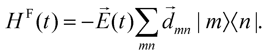 | (11) |
E(t) = E0![[thin space (1/6-em)]](https://www.rsc.org/images/entities/char_2009.gif) cos(ωt)exp(−(t − t0)2/2σ2) cos(ωt)exp(−(t − t0)2/2σ2) | (12) |
 .
.
2.3 ML-MCTDH method
 | (13) |
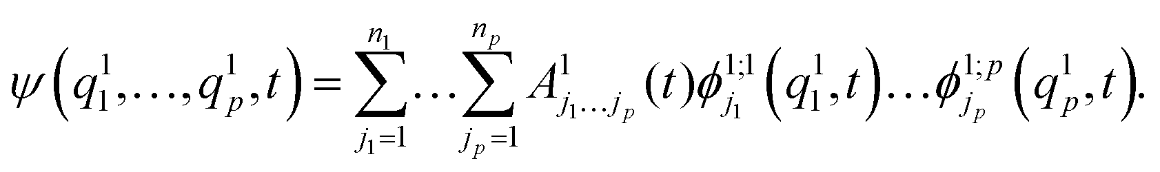 | (14) |
 are multi-dimensional SPFs for the κth particle (number of SPFs is nκ). Within a three-layer scheme in the second layer the multi-dimensional SPFs, ϕ1;κλ(q1κ,t), are fully unraveled into SPFs for the physical coordinates and expanded according to
 | (15) |
 | (16) |
The extension to more layers is straightforward. In this case, each layer introduces a new set of logical coordinates, each derived from a subset of the coordinates combined in the preceding layer. The resulting structure of the wave packets can be visualized using so-called ML-trees.46 Equations of motion for SPFs and coefficient vectors can be obtained by applying the Dirac–Frenkel time-dependent variational principle.47 Convergence can be controlled by inspecting the so-called natural orbital populations related to the SPFs. Below we will define thresholds for the largest population of the least occupied natural orbital, pNO.
Finally, we note that the limit where the wavepacket ψm(Q,t) is expressed as a simple Hartree product for all physical coordinates is called the time-dependent Hartree (TDH) approach.
 | (17) |
Next, we define the adjacency matrix W of an associated weighted graph with matrix elements
| Wξξ′ = |Cξξ′| − δξξ′. | (18) |
In this work, we relied on a spectral clustering algorithm,50,68–71 in contrast to ref. 49 which used hierarchical clustering. How the two methods compare in the context of ML-MCTDH efficiency will require further investigation. We prefer spectral clustering as it provides a means to directly control the size of the clusters, which will be important for the discussion below. In addition, it circumvents the problem of predefining a metric that dictates the structure of the obtained dendrogram in hierarchical clustering. In short, spectral clustering proceeds as follows. First, the symmetrized Laplacian is computed, for which the lowest k eigenvalues and eigenvectors are determined. Afterward, each row of the matrix, whose columns are the eigenvectors, is treated as a data point. Data points are grouped into k clusters using k-means. Given a clustering at the level of the full correlation matrix, the procedure is repeated until subclusters of either size one or two are obtained.
The final result is a ML-tree for which the number of SPFs at each vertex has to be obtained. This is done by iteratively propagating the equations of motion while increasing the number of SPFs until a predefined threshold for pNO has been reached. For the specific examples below this was done in the time interval [0:1000 fs].
3 Computational details
The flowchart of the computational protocol is provided in Fig. 2: (1) a BSE@GW calculation of vertical excitation energies is performed for a given geometry. (2) LVC parameters are obtained according to eqn (7) and (8). Using these parameters the diabatic Hamiltonian is constructed and a full-dimensional TDH dynamics simulation is performed for a given laser field (3). Based on the time-dependent expectation values of the normal mode coordinate, the (Pearson) correlation matrix C is determined (4). If desired, the number of DOFs can be reduced, e.g. by inspecting the magnitude of coordinate displacements. Using spectral clustering (5), a ML-tree is generated as input for ML-MCTDH simulations. Simulations are performed with systematically adapted numbers of SPFs until a given convergence criterion in terms of natural orbital populations (pNO) is met (6). Having a converged setup, the dynamics can be analyzed, e.g. in terms of electronic state populations (7).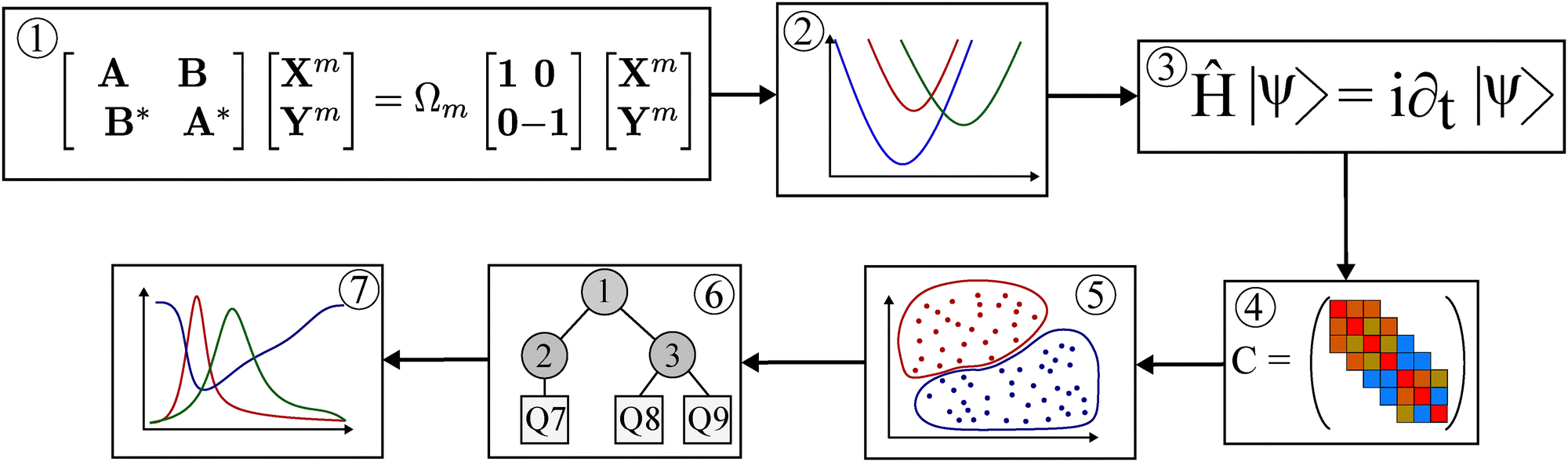 | ||
| Fig. 2 Flowchart of the simulation protocol used in this work. BSE@GW computations (1) are used as input to generate an LVC model for the entire diabatic PES as a function of normal mode displacement coordinates (2). Wave packets are propagated on this model in TDH approximation (3) to compute the correlation matrix of coordinate expectation values (4). The clustering of the resulting adjacency matrix (5) generates an ML-tree (6), which serves as the input for executing ML-MCTDH dynamics simulations to obtain electronic state populations as a function of time (7). | ||
All quantum chemical calculations were performed using TURBOMOLE version 7.8.1.72,73 In particular, the BSE@GW and TD-DFT calculations were done with the ESCF module74,75 using the TDA. Self-consistent field calculations were performed in the RIDFT76 module, making use of the resolution of identity (RI) approximation. SOC matrix elements were calculated with TURBOMOLE's PROPER module using the effective one-electron operator option, which includes a screened nuclear charge.64,77 The range-separated functional LC-BLYP was used with parameters taken from ref. 13. The equilibrium geometry was obtained through DFT geometry optimization using the LC-BLYP (α = 0.2, ω = 0.08) functional, which resulted in a C2 symmetric structure, although symmetry was not enforced and has not explicitly been used in subsequent calculations.
All calculations were performed using a def2-TZVP basis set. The auxiliary basis sets (jbas and cbas) were always of the same quality as the regular ones. Convergence criteria were set to $scfconv = 7 and $rpaconv = 5. The m5 grid option was always chosen. UV-Vis spectra were computed by broadening vertical transition energies by a Lorentzian function with a full-width-half-maxima of 0.25 eV. The length gauge was always chosen as the height of the absorption peak. The analysis of the transition density matrices was performed with the THEODORE program package version 3.2.78,79
All calculations regarding the LVC model were carried out in a modified version of the SHARC 3.0 program package.14,80 To do so, a new interface between SHARC and TURBOMOLE's ESCF/PROPER module was developed, which follows the established SHARC routines. It enables one to carry out a full LVC parametrization32 of the PES using both the BSE@GW and TD-DFT levels of theory. The computation of the overlap matrix was also performed in SHARC's WFOVERLAP module.66 Our LVC model included the lowest 10 singlet (including the singlet ground state) and 14 triplet states. This covers the range of excitation energies up to about 2.5 eV, thus enabling a comparison with the transient absorption experiments conducted to study the MLCT states in this range and reported in ref. 13. We opted for a def2-TZVP basis set as we observed that the BSE@GW calculations demonstrate a high sensitivity to basis set quality (see Fig. S1 in the ESI†). Both the RI and TDA were employed and the first 49 core molecular orbitals were discarded to calculate the wave function overlaps. A wave function truncation threshold of 0.998 was chosen. The same convergence criteria and grid settings for the BSE@GW calculations were chosen as those used for the spectra calculations. For this model, we used a displacement factor of 0.05. To calculate the GW quasiparticle energies, contour deformation techniques (CD)81–83 were used with an orbital range of [157,177] for which the correlation part of the self-energy was calculated. The eigenvalue-only self-consistent GW scheme (evGW) was used to converge quasiparticle energies. The range-separated functional LC-BLYP (α = 0.2, ω = 0.08) was taken as a starting point.
ML-MCTDH computations were performed with the Heidelberg MCTDH package Version 8.6.5.35,36,84,85 For the primitive basis in eqn (16) a ten-point harmonic oscillator discrete variable representation was used. The equations of motion were solved employing variable mean fields, together with a 5th-order Runge–Kutta solver. The ML-trees were generated using spectral clustering as implemented in ref. 86.
All computations were performed on an Intel Xeon Gold 6326 CPU@2.90 GHz, which served as the benchmark system for comparing the computational demand of the different calculation setups.
4 Results and discussion
In what follows we will separate our discussion into two parts. First, we will focus on static properties, such as the ground state absorption spectrum and the general structure of the PES. For this, we aim at comparing the BSE@GW framework to TD-DFT and highlight important differences in the obtained results. In this part, we will also present the LVC parametrization of the molecular Hamiltonian based on BSE@evGW.Second, we will perform ML-MCTDH quantum dynamics simulations using the obtained LVC Hamiltonian. Here, the emphasis will be put on the performance of the spectral clustering algorithm for ML-tree generation.
4.1 Assignment of the absorption spectrum
Vertical absorption spectra in the singlet ground state geometry were computed using BSE@evGW as well as TD-DFT with different LC-BLYP parameters. Results are compared in Fig. 3, where also experimental data are given.51 In terms of TD-DFT, the best alignment of the computed spectrum is obtained for the (α = 0, ω = 0.14) parameter set. In this instance, all three absorption peaks are close to the experimental values. In addition, their oscillator strengths also appear to be reasonably accurate. The agreement with the experiment is rather sensitive to the tuning parameters. For instance, an increase of the exact exchange at short distances (α) leads to a deterioration of the alignment, in the sense that the lower two peaks are shifted towards higher energies, and the one at the higher energy is losing a significant amount of its oscillator strength. These findings align well with previous results for this system, where the same trend was observed.13 In ref. 13 it was also shown that the parameter set (α = 0.2, ω = 0.08), although not showing the best performance in terms of the absorption spectrum, gives a much better description of the dynamics after photoexcitation. | ||
| Fig. 3 Absorption spectra, according to TD-DFT and BSE@GW using the LC-BLYP functional for different α and ω values. The gray-shaded area refers to the experimental data from ref. 51. | ||
In contrast, the BSE@evGW framework provides an improvement of the absorption spectrum when comparing with the TD-DFT results for (α = 0.2, ω = 0.08), albeit it does not perform as well as the TD-DFT (α = 0, ω = 0.14) protocol. At first glance this appears disappointing, particularly recalling the superior performance for similar Fe-compounds reported in ref. 27. In that work, it was also shown that there is only a small dependence of the BSE@GW spectra on the XC-functional, implying for the present case that along this line there is perhaps little room for improvement of the result shown in Fig. 3. In fact, the only variable to impact the resulting spectra appears to be the amount of exact exchange used as seen in the ESI,† Fig. S12 and S13.
However, the correct reproduction of the absorption spectrum is only one part of the picture. In addition, the CT characters must also be described properly, to obtain an accurate characterization of the underlying electronic transitions. To scrutinize this point, an analysis of the TDM was performed for the singlet and triplet excitations contributing to the absorption spectrum in Fig. 3. Here the singlet ground state geometry was assumed. We will compare the order of the states with CASPT2 results on the lowest excitations, which gave for singlets/triplets that the MLCT transitions is energetically below/above the MC one.13 Note that in ref. 13 the active space was designed with a focus on the lowest singlet and triplet transitions only. That is, there is no CASPT2 grade information on the absorption spectrum and its assignment.
The results in Fig. 4 show that LC-BLYP (α = 0, ω = 0.14) provides a reasonable description of the absorption spectrum, even though it incorrectly predicts the ordering of the excited triplet states, placing the MLCT state below the MC state, which does not align with previous CASPT2 computations.13 In fact, an increase of the short-range exact exchange contribution (α) is required to obtain the correct ordering, which simultaneously worsens the alignment with the experiments. Further, it bears the risk of overcompensation up to the point where the MC states are placed below the MLCT in the singlet absorption spectrum. We obtained the correct ordering of the lowest MLCT/MC transitions for the parameters (α = 0.1, ω = 0.11).
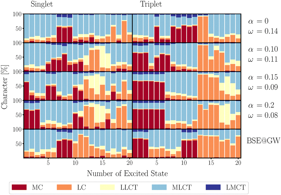 | ||
| Fig. 4 Analysis of the singlet and triplet TDM for the different tuning parameters and methods used in Fig. 3. The geometry corresponds to a vertical excitation from the singlet ground state. Note that the pronounced mixing a MC and MLCT states evidences the deviation from octahedral symmetry of this complex. Numerical values for transition energies are given in Tables S1 and S2 of the ESI.† | ||
In comparison, BSE@evGW yields the correct ordering in both the lowest singlet and triplet states without requiring the separate tuning of parameters, aligning well with observations for similar systems.27 This advantage of the BSE@GW framework over TD-DFT motivates its usage as a basis to construct an LVC model and perform subsequent dynamics simulations.
4.2 LVC parametrization
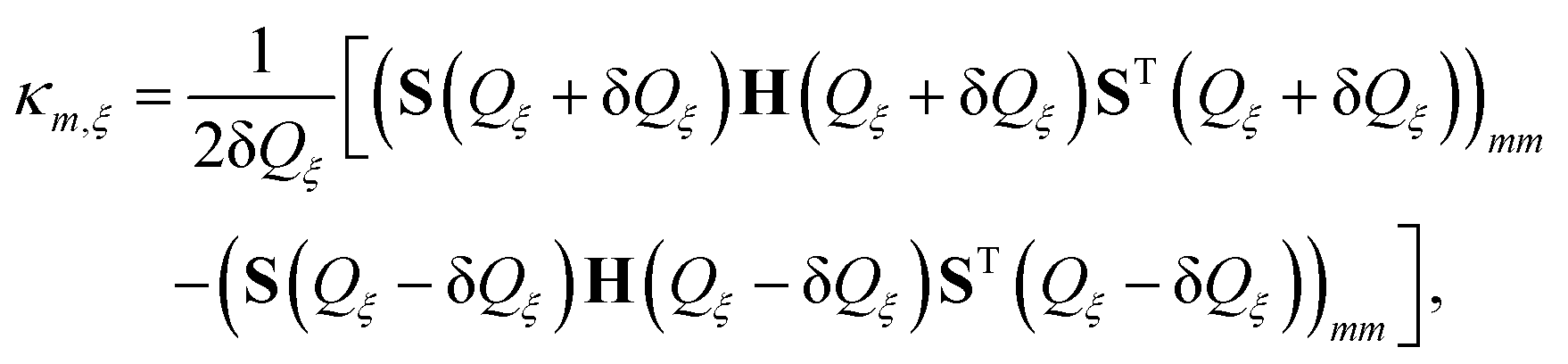
An LVC parametrization of the full-dimensional (213 normal modes) diabatic Hamiltonian was performed using the method described in Section 2.2. The resulting LVC Hamiltonian contains a set of 5112 κ and 28968 λ values (excluding the degeneracy of the triplet states). A large number of these values is rather small. In order to reduce the number of operator terms in the MCTDH setup, we have defined a threshold of 1 meV for inclusion into the ML-MCTDH simulation. The same holds for the SOC, which in total contains 840 terms. Using the threshold the number of terms reduces to 2768, 11089, and 408 for κ, λ, and the SOC matrix elements, respectively.
A histogram of these obtained values is given in Fig. 5. It shows that most of the coupling constants are small, i.e. below about 0.07 eV for κ and λ and below about 0.025 eV for SOC. While this is comparable to the TD-DFT results reported in ref. 52, the majority of κ values are a bit larger (below about 0.12 eV) in TD-DFT. Above the mentioned values, some scattered coupling parameters do not have exact counterparts in TD-DFT. Notice that the TD-DFT results had been obtained using LC-BLYP (α = 0.2, ω = 0.08), which according to our discussion in the previous section (cf.Fig. 4) shows a different composition of transitions as compared with BSE@evGW. This will have, of course, an influence on the coupling parameters, in accordance with the present findings. For instance, the MC character will be reflected in the shift of the PES. In light of the discussion of Fig. 5, which concluded on a more robust description of the character of transitions by BSE@evGW, the κ and λ values should be considered more reliable than the published TD-DFT ones.52
 | ||
| Fig. 5 Histogram of absolute values of all (a) κm,ξ, (b) λmn,ξ and (c) SOC constants. In the Hamiltonian used for ML-MCTDH propagation all couplings with absolute values below 0.001 eV were discarded. | ||
It is interesting to ask whether the LVC model itself is applicable. The general quality of the κ and λ parameters can be estimated by comparing the resulting adiabatic PES (obtained by diagonalization of the LVC Hamiltonian) with single-point calculations for a set of geometries, displaced along particular normal modes. In Fig. 6 respective PES cuts along the mode with ξ = 25 having a frequency of 186 cm−1 are shown. It is a symmetric breathing mode meaning that a positive displacement corresponds to an elongation of the Fe–N bond lengths (results for other modes can be found in the ESI,† Fig. S2).
 | ||
| Fig. 6 Comparison between adiabatic PES cuts along mode ξ = 25 (breathing mode) obtained via explicit single point calculations (dots) and in LVC approximation. In the latter case, the blue continuous lines show singlet, whereas the red dashed lines refer to tripet states. Panel (a) and (b) show the PES for BSE@evGW and (c) and (d) for TD-DFT. Both calculations made use of the LC-BLYP (α = 0.2, ω = 0.08) functional. The energy axis is shifted, such that the S0 groundstate at q = 0 is set 0 eV. | ||
Overall, one observes that the calculated LVC PES, as obtained with BSE@evGW (Fig. 6(a, b)) as well as TD-DFT (Fig. 6(c, d)), decently align with the single-point calculations, especially around the equilibrium geometry, where the PES show harmonic characteristics (for a more anharmonic case, see Fig. S2(a) in ESI†). In particular, we observe a good agreement for the lowest triplet states, which are often difficult to describe properly. Besides the fairly good performance of the LVC approximation as such, the PES of BSE@evGW and TD-DFT show distinct differences. For instance, the lowest excited singlet state potential curve is considerably more displaced (large κ) in TD-DFT as compared with BSE@evGW. This is not surprising given the fact that according to Fig. 4, TD-DFT predicts a dominant MC (anti-bonding) character. The displacement of the potential curve for the lowest triplet state, on the other hand, is rather similar in BSE@evGW and TD-DFT, in accord with its comparable character in Fig. 4. Finally, we notice that BSE@evGW predicts a higher density of states in this energy range as compared with TD-DFT.
As has been highlighted for the case of TD-DFT and different LC-BLYP tuning parameters in ref. 13 already, differences in coupling parameters can lead to rather different dynamics, even though the absorption spectra are similar. We will not further elaborate on a comparison of BSE@evGW and TD-DFT in terms of the quantum dynamics. Instead, the focus of the next section will be on general aspects of the performance of the ML-tree generation using spectral clustering.
4.3 ML-MCTDH wave packet dynamics simulations
With the full LVC Hamiltonian at hand, TDH dynamics simulations were performed for 2000 fs with the dynamics being triggered by a field according to eqn (12). The field was assumed to be polarized along the direction of the y-component of the dipole (direction with largest transition dipole) and resonant to the strongest transition in the low-energy MLCT band (ω = 2.34 eV). Furthermore, we used t0 = 100 fs, σ = 24 fs, and E0 = 0.001 hartree bohr−1. These values gave a ground state depopulation of about 27%. Since our focus is on the ML-tree generation, a model of reduced dimensionality has been selected. Specifically, we included only those modes with a maximum absolute coordinate expectation value larger than 0.15. This resulted in a 63-dimensional model with 755 and 3895 terms for κ and λ, respectively. The population dynamics of this model is qualitatively similar to that of the full-dimensional case. The obtained adjacency matrix, eqn (18), is shown in Fig. 7. There, one can identify sets of normal modes which appear to be highly correlated. Visually, one might initially group modes based on the fact that modes that are close in energy usually demonstrate a strong correlation. However, the presence of significant off-diagonal elements indicate that not only modes that are close in energy may show a strong correlation. As mentioned in the introduction, we therefore used a spectral clustering algorithm to divide the adjacency matrix W into smaller subsets, which consequently takes into account entries that are located far away from the main diagonal. | ||
| Fig. 7 Heatmap of the adjacency matrix W for the 63-dimensional LVC model. The color of the element Wξ,ξ′ refers to the Pearson correlation value between normal modes Qξ and Qξ′. The counting of vibrational normal modes starts at seven and only every third mode number is given for readability. | ||
Based on this procedure, we generated five different trees for detailed investigation. All trees are shown in the ESI,† Fig. S3–S8. The first four were binary trees, where W was decomposed into two clusters in each layer, but with a varying threshold for entries. In this instance, we have chosen the four thresholds ΔW 0 (I), 0.1 (II), 0.2 (III), and 0.3 (IV). Entries of W that fell below these values were set to 0 accordingly, meaning that the two modes are considered uncorrelated. In principle, a small threshold will give a larger set of isolated modes, leading the clustering algorithm to generate a deeper ML-tree (cf. ESI,† Fig. S3–S6). This occurs because the likelihood increases that, at a specific node, the clustering algorithm groups a small set of normal modes into one branch, while passing the majority of normal modes further down to the next layer. This way a small threshold in the adjacency matrix may be seen as a tool to deepen the ML-tree by choice. However, increasing the threshold could lead to a situation where most entries of the adjacency matrix are located around the diagonal. This may aid the spectral clustering algorithm in identifying highly correlated pairs and thus reducing the depth of the ML-tree (cf. ESI,† Fig. S6). For the present models (I) to (IV) we have 10, 11, 18, and 17 layers, respectively. In general, having deeper ML-trees could be desirable as related research has shown that this may lead to a lower computational effort.87 However, at the same time, this could increase the number of SPFs, which may counterbalance the positive effect on efficiency. The remaining tree (V) was chosen such that the full adjacency matrix was divided into clusters of different sizes. The first layer was decomposed into 3 clusters, followed by two for all remaining layers. Of course, the present choice of ML-trees is just a subset of in principle possible trees, picked by intuition and serving the purpose of comparison.
Below we will discuss the performance and convergence of the different ML-trees in terms of the total (singlet + triplet) MLCT population. The connection to the overall dynamics is provided in Fig. 8. These results were obtained with tree (IV), which gave the best performance as will be detailed below. In Fig. 8 one observes the expected behavior for this type of system. Initially, the laser pulse excited the 1MLCT states which rapidly convert into 3MLCT states due to intersystem crossing. Internal conversion subsequently leads to a population relaxation in the triplet manifold towards the low-lying 3MC states. Depopulation of MLCT states in the excitation window takes place within a few hundred femtoseconds, which is in accord with the experimental observation by Moll et al.51 In passing we note that the states with the highest energy in the given interval are only marginally populated, thus giving support for the restriction to 10 singlet and 14 triplet states for the given excitation conditions.
 | ||
| Fig. 8 Energy-resolved ML-MCTDH population dynamics of diabatic spin-free states for the 63-dimensional LVC model and for tree (IV) with pNO converged to 0.2%. | ||
In what follows, the convergence behaviour of the five ML-trees is investigated by gradually decreasing the threshold for pNO. In Fig. 9(a) the total MLCT population for tree (IV) is shown for pNO ranging from 5% to 0.2%. Only minor differences are observed between the two curves with the tightest convergence criteria. We therefore take the curve with the tightest convergence criteria as a reference to compare them against the remaining models. It is interesting to note that only the reference calculation reproduces dynamics in accordance with what would be expected for this type of system. In contrast, higher convergence thresholds lead to oscillations as well as long-lived populations in the higher-lying excited triplet states (for an example, see ESI,† Fig. S1).
 | ||
| Fig. 9 Convergence behavior for MLCT diabatic populations for models (a) (IV), (b) (I), and (c) (V). The graphs are labeled according to the convergence threshold set pNO × 1000. The tightest convergence criteria for model (IV) of 0.2% will be set as a reference. Notice that in all curves there is a slight initial rise, which is discussed in ESI,† Section S7. | ||
The required convergence threshold and the speed at which convergence is achieved depend strongly on the structure of the ML-tree. This can be seen by comparing the different panels of Fig. 9. In all cases, the not sufficiently converged results show a slower decay of the MLCT population, i.e. in particular a trapping of population in high-lying excited triplet states. Increasing the convergence threshold will lead to the dynamics trending towards the reference results, although with varying speeds (to make sure that this is not a feature of the particular model, it has been checked for a 42-dimensional model, see ESI,† Fig. S11).
It appears that even the tightest convergence thresholds used remain insufficient for model (I), as rather large changes are observed. The same behavior can be observed for systems (II) and (III), which all appear to converge slower than (IV) (cf. ESI,† Fig. S9). Thus we can conclude that deepening of the ML-tree structure by setting a threshold for the adjacency matrix may indeed improve convergence with respect to pNO, but at the time being it is not clear whether there is an optimal choice. Model (V) (having a comparatively flat tree) in Fig. 9(c) demonstrated by far the highest computational demand, combined with the slowest convergence behavior. In passing, we note that an ML-tree with 4 clusters at the top, followed by 3 in the second layer and 2 for all remaining ones was also tested. However, the convergence was too slow and the computational demand too high to obtain results in a time comparable to all other models.
The CPU time requirement of all ML-trees is shown in Fig. 10. Here, we notice that all binary ML-trees result in a comparable computational demand at a given threshold pNO. This observation should be highlighted in particular, as the ML-trees of the first four models have a completely different structure and, depending on the depth of the structure, a significantly higher amount of SPFs (see ESI,† Fig. S3–S8). We conclude that a binary ML-tree structure should consequently be preferred over other related structures for this system to achieve a reliable low computational cost, as all results trend toward the converged reference calculation with comparable computational cost.
 | ||
| Fig. 10 CPU time of the different ML-tree structures for different convergence thresholds. All results are normalized to the model (IV) simulation for a threshold of pNO = 0.5%. | ||
5 Conclusions
We have presented a new computational toolbox, combining the calculation of BSE@evGW based LVC model Hamiltonians and automated tree generation for ML-MCTDH wave packet simulations. The workflow makes use of the newly developed SHARC-ESCF (TURBOMOLE) interface for BSE@GW calculations of adiabatic electronic wave function overlaps. This yields an LVC parametrization to define a sum-of-products Hamiltonian suitable for ML-MCTDH. This Hamiltonian is used to perform TDH simulations which provides a correlation matrix of coordinate expectation values. The related adjacency matrix serves as input for a spectral clustering algorithm yielding ML-trees whose structure can be influenced, e.g. by setting thresholds for the adjacency matrix. Different ML-trees may generally result in vastly different efforts for obtaining convergence with respect to the number of SPFs entering the wave packet expansion. Due to the variational nature of the ML-MCTDH ansatz different trees should upon convergence yield the same dynamics.The new protocol was applied to the photoinduced dynamics of an Fe(II) complex. Here it should be noted that BSE@evGW gave a reasonable absorption spectrum if compared with experiment and TD-DFT using an optimized LC-BLYP functional. More importantly and in contrast to TD-DFT, however, BSE@evGW provided a reasonable assignment of the lowest singlet and triplet transitions. Since the characters of transitions determine vibronic couplings, the BSE@evGW derived LVC parameters can be considered superior if compared to TD-DFT. ML-MCTDH dynamics after pulsed excitation yielded results for the MLCT populations in accord with experiment. The performance of different ML-trees was rather different in terms of convergence with respect to the number of SPFs and associated computational demands. Although there is not yet a strict method for tree optimization, for the present case it has been shown that spectral clustering with binary trees and using a threshold for the adjacency matrix leads to efficient ML-MCTDH setups.
The investigated transition metal complex can be considered a challenging case in terms of electronic structure and dimensionality of spin-vibronic dynamics. This suggests that the presented protocol should be applicable to a broad range of molecular systems.
Conflicts of interest
There are no conflicts to declare.Data availability
All data are available from the authors upon reasonable request. The SHARC interface to escf used in this work is available on Github https://github.com/bogdainflorian/SHARCESCF. The interface will be fully integrated into the SHARC package in a future release.Acknowledgements
This work is funded by the Deutsche Forschungsgemeinschaft (DFG, German Research Foundation) – SFB 1477 “Light-Matter Interactions at Interfaces”, project number 441234705, and via the projects GO 1059/8-2 and KU 952/12-2 within the SPP 2102 “Light-Controlled Reactivity of Metal Complexes”, project number 403837698. The authors thank A. Kruse and M. A. Argüello Cordero (University of Rostock) for providing the experimental data. LG and SM acknowledge the Vienna Scientific Cluster (VSC5) for generous allocation of computational resources and the University of Vienna for continuous support.Notes and references
- T. J. Penfold, E. Gindensperger, C. Daniel and C. M. Marian, Chem. Rev., 2018, 118, 6975–7025 CrossRef CAS PubMed.
- O. S. Wenger, Chem. – Eur. J., 2019, 25, 6043–6052 CrossRef CAS PubMed.
- J. K. McCusker, Science, 2019, 363, 484–488 CrossRef CAS PubMed.
- P. Chábera, L. Lindh, N. W. Rosemann, O. Prakash, J. Uhlig, A. Yartsev, K. Wärnmark, V. Sundström and P. Persson, Coord. Chem. Rev., 2021, 426, 213517 CrossRef.
- K. J. Gaffney, Chem. Sci., 2021, 12, 8010–8025 RSC.
- J. Steube, A. Kruse, O. S. Bokareva, T. Reuter, S. Demeshko, R. Schoch, M. A. Argüello Cordero, A. Krishna, S. Hohloch and F. Meyer, et al. , Nat. Chem., 2023, 15, 468–474 CrossRef CAS PubMed.
- C. Daniel, Phys. Chem. Chem. Phys., 2021, 23, 43–58 RSC.
- L. Lindh, P. Chábera, N. W. Rosemann, J. Uhlig, K. Wärnmark, A. Yartsev, V. Sundström and P. Persson, Catalysts, 2020, 10, 315 CrossRef CAS.
- S. I. Bokarev, O. S. Bokareva and O. Kühn, Coord. Chem. Rev., 2015, 304–305, 133–145 CrossRef CAS.
- S. Kümmel, Adv. Energy Mater., 2017, 7, 1700440 CrossRef.
- O. S. Bokareva, G. Grell, S. I. Bokarev and O. Kühn, J. Chem. Theory Comput., 2015, 11, 1700–1709 CrossRef CAS PubMed.
- O. S. Bokareva, O. Baig, M. J. Al-Marri, O. Kühn and L. González, Phys. Chem. Chem. Phys., 2020, 22, 27605–27616 RSC.
- J. P. Zobel, A. Kruse, O. Baig, S. Lochbrunner, S. I. Bokarev, O. Kühn, L. González and O. S. Bokareva, Chem. Sci., 2023, 14, 1491–1502 RSC.
- S. Mai, P. Marquetand and L. Gonzalez, Wiley Interdiscip. Rev.:Comput. Mol. Sci., 2018, 8, e1370 Search PubMed.
- X. Blase, I. Duchemin, D. Jacquemin and P.-F. Loos, J. Phys. Chem. Lett., 2020, 11, 7371–7382 CrossRef CAS PubMed.
- M. Dvorak, B. Baumeier, D. Golze, L. Leppert and P. Rinke, Front. Chem., 2022, 10, 866492 CrossRef PubMed.
- I. Knysh, K. Letellier, I. Duchemin, X. Blase and D. Jacquemin, Phys. Chem. Chem. Phys., 2023, 25, 8376–8385 RSC.
- Z. Hashemi, M. Knodt, M. R. Marques and L. Leppert, Electron. Struct., 2023, 5, 024006 CrossRef CAS.
- T. Biswas and A. K. Singh, npj Comput. Mater., 2023, 9, 22 CrossRef.
- X. Leng, F. Jin, M. Wei and Y. Ma, Wiley Interdiscip. Rev.:Comput. Mol. Sci., 2016, 6, 532–550 CAS.
- L. Leppert, J. Chem. Phys., 2024, 160, 050902 CrossRef CAS PubMed.
- S. Bhattacharya, J. Li, W. Yang and Y. Kanai, J. Phys. Chem. A, 2024, 128, 6072–6083 CrossRef CAS PubMed.
- M. L. Tiago and J. R. Chelikowsky, Solid State Commun., 2005, 136, 333–337 CrossRef CAS.
- L. Hung, F. H. da Jornada, J. Souto-Casares, J. R. Chelikowsky, S. G. Louie and S. Öğüt, Phys. Rev. B, 2016, 94, 085125 CrossRef.
- C. Holzer and W. Klopper, J. Chem. Phys., 2019, 150, 204116 CrossRef PubMed.
- I. Knysh, F. Lipparini, A. Blondel, I. Duchemin, X. Blase, P.-F. Loos and D. Jacquemin, J. Chem. Theory Comput., 2024, 20, 8152–8174 CAS.
- F. Bogdain and O. Kühn, J. Chem. Theory Comput., 2025, 21, 4494 CrossRef CAS PubMed.
- H. Köppel, W. Domcke and L. S. Cederbaum, Multimode Molecular Dynamics Beyond the Born-Oppenheimer Approximation, John Wiley and Sons, Ltd, 1984, pp. 59–246 Search PubMed.
- O. Kühn and V. May, Charge and Energy Transfer Dynamics in Molecular Systems, Wiley-VCH, Weinheim, 2023 Search PubMed.
- O. Çaylak and B. Baumeier, J. Chem. Theory Comput., 2021, 17, 879–888 CrossRef PubMed.
- F. Plasser, S. Gómez, M. F. S. J. Menger, S. Mai and L. González, Phys. Chem. Chem. Phys., 2019, 21, 57–69 RSC.
- M. Fumanal, F. Plasser, S. Mai, C. Daniel and E. Gindensperger, J. Chem. Phys., 2018, 148, 124119 CrossRef PubMed.
- J. P. Zobel and L. González, JACS Au, 2021, 1, 1116–1140 CrossRef CAS PubMed.
- S. Polonius, O. Zhuravel, B. Bachmair and S. Mai, J. Chem. Theory Comput., 2023, 19, 7171–7186 CrossRef CAS PubMed.
- H.-D. Meyer, U. Manthe and L. Cederbaum, Chem. Phys. Lett., 1990, 165, 73–78 CrossRef CAS.
- M. Beck, A. Jäckle, G. Worth and H.-D. Meyer, Phys. Rep., 2000, 324, 1–105 CrossRef CAS.
- G. A. Worth, H.-D. Meyer, H. Köppel, L. S. Cederbaum and I. Burghardt, Int. Rev. Phys. Chem., 2008, 27, 569–606 Search PubMed.
- J. Eng, C. Gourlaouen, E. Gindensperger and C. Daniel, Acc. Chem. Res., 2015, 48, 809–817 CrossRef CAS PubMed.
- M. Pápai, J. Chem. Theory Comput., 2022, 18, 1329–1339 CrossRef PubMed.
- J. Schulze and O. Kühn, J. Phys. Chem. B, 2015, 119, 6211–6216 CrossRef CAS PubMed.
- J. Schulze, M. F. Shibl, M. J. Al-Marri and O. Kühn, J. Chem. Phys., 2016, 144, 185101 CrossRef PubMed.
- O. Vendrell, F. Gatti and H.-D. Meyer, Angew. Chem., Int. Ed., 2007, 46, 6918 CrossRef CAS PubMed.
- H. Naundorf, G. A. Worth, H.-D. Meyer and O. Kühn, J. Phys. Chem. A, 2002, 106, 719–724 CrossRef CAS.
- H.-D. Meyer and F. Gatti, Multidimensional Quantum Dynamics: MCTDH Theory and Applications, Wiley-VCH, Weinheim, 2009 Search PubMed.
- H. Wang and M. Thoss, J. Chem. Phys., 2003, 119, 1289–1299 CrossRef CAS.
- U. Manthe, J. Chem. Phys., 2008, 128, 164116 CrossRef PubMed.
- O. Vendrell and H.-D. Meyer, J. Chem. Phys., 2011, 134, 044135 CrossRef PubMed.
- M. Schröter, S. D. Ivanov, J. Schulze, S. P. Polyutov, Y. Yan, T. Pullerits and O. Kühn, Phys. Rep., 2015, 567, 1–78 CrossRef.
- D. Mendive-Tapia, H.-D. Meyer and O. Vendrell, J. Chem. Theory Comput., 2020, 19, 1144–1156 CrossRef PubMed.
- U. von Luxburg, Stat. Comput., 2007, 17, 395–416 CrossRef.
- J. Moll, R. Naumann, L. Sorge, C. Förster, N. Gessner, L. Burkhardt, N. Ugur, P. Nuernberger, W. Seidel, C. Ramanan, M. Bauer and K. Heinze, Chem. – Eur. J., 2022, 28, e202201858 CrossRef CAS PubMed.
- O. S. Bokareva and O. Kühn, in Comprehensive Computational Chemistry, ed. M. Yanez and R. Boyd, Elsevier, Oxford, 2024, vol. 4, p. 385 Search PubMed.
- C. Holzer, PhD thesis, Karlsruhe Institute of Technology, 2018.
- A. Förster and L. Visscher, J. Chem. Theory Comput., 2022, 18, 6779–6793 CrossRef PubMed.
- G. Strinati, Rev. Nuovo Cimento, 1988, 11, 1–86 CrossRef CAS.
- L. Hedin, Phys. Rev., 1965, 139, A796–A823 CrossRef.
- M. E. Casida, J. Mol. Struct. THEOCHEM, 2009, 914, 3–18 CrossRef CAS.
- F. Furche, J. Chem. Phys., 2001, 114, 5982–5992 CrossRef CAS.
- S. Hirata and M. Head-Gordon, Chem. Phys. Lett., 1999, 314, 291–299 CrossRef CAS.
- F. Gatti, B. Lasorne, H. D. Meyer and A. Nauts, Applications of Quantum Dynamics in Chemistry, Springer, Cham, 2017 Search PubMed.
- S. M. Parker, D. Rappoport and F. Furche, J. Chem. Theory Comput., 2018, 14, 807–819 CrossRef CAS PubMed.
- N. Rauwolf, W. Klopper and C. Holzer, J. Chem. Phys., 2024, 160, 061101 CrossRef CAS PubMed.
- X. Gao, S. Bai, D. Fazzi, T. Niehaus, M. Barbatti and W. Thiel, J. Chem. Theory Comput., 2017, 13, 515–524 CrossRef CAS PubMed.
- P. Himmelsbach and C. Holzer, J. Chem. Phys., 2024, 161, 244105 CrossRef CAS PubMed.
- D. Farkhutdinova, S. Polonius, P. Karrer, S. Mai and L. González, J. Phys. Chem. A, 2025, 129, 2655–2666 CrossRef CAS PubMed.
- F. Plasser, M. Ruckenbauer, S. Mai, M. Oppel, P. Marquetand and L. González, J. Chem. Theory Comput., 2016, 12, 1207–1219 CrossRef CAS PubMed.
- F. Plasser, M. Wormit and A. Dreuw, J. Chem. Phys., 2014, 141, 024106 CrossRef PubMed.
- J. Shi and J. Malik, IEEE Trans. Pattern Anal. Mach. Intell., 2000, 22, 888–905 CrossRef.
- A. Ng, M. Jordan and Y. Weiss, Advances Neural Inf. Process. Syst., 2001, 14, 849–856 Search PubMed.
- H. Jia, S. Ding, X. Xu and R. Nie, Neural Comput. Appl., 2013, 24, 1477–1486 CrossRef.
- J. Liu and J. Han, Data clustering, Chapman and Hall/CRC, 2018, pp. 177–200 Search PubMed.
- TURBOMOLE V7.8 2023, a development of University of Karlsruhe and Forschungszentrum Karlsruhe GmbH, https://www.turbomole.org, 1989–2007.
- S. G. Balasubramani, G. P. Chen, S. Coriani, M. Diedenhofen, M. S. Frank, Y. J. Franzke, F. Furche, R. Grotjahn, M. E. Harding, C. Hättig, A. Hellweg, B. Helmich-Paris, C. Holzer, U. Huniar, M. Kaupp, A. Marefat Khah, S. Karbalaei Khani, T. Müller, F. Mack, B. D. Nguyen, S. M. Parker, E. Perlt, D. Rappoport, K. Reiter, S. Roy, M. Rückert, G. Schmitz, M. Sierka, E. Tapavicza, D. P. Tew, C. van Wüllen, V. K. Voora, F. Weigend, A. Wody'ski and J. M. Yu, J. Chem. Phys., 2020, 152, 184107 CrossRef CAS PubMed.
- M. J. van Setten, F. Weigend and F. Evers, J. Chem. Theory Comput., 2013, 9, 232–246 CrossRef CAS PubMed.
- K. Krause and W. Klopper, J. Comput. Chem., 2017, 38, 383–388 CrossRef CAS PubMed.
- O. Treutler and R. Ahlrichs, J. Chem. Phys., 1995, 102, 346–354 CrossRef CAS.
- S. G. Chiodo and M. Leopoldini, Comput. Phys. Commun., 2014, 185, 676–683 CrossRef CAS.
- F. Plasser, J. Chem. Phys., 2020, 152, 084108 CrossRef CAS PubMed.
- F. Plasser and H. Lischka, J. Chem. Theory Comput., 2012, 8, 2777–2789 CrossRef CAS PubMed.
- S. Mai, D. Avagliano, M. Heindl, P. Marquetand, M. F. S. J. Menger, M. Oppel, F. Plasser, S. Polonius, M. Ruckenbauer, Y. Shu, D. G. Truhlar, L. Zhang, P. Zobel and L. Gonzalez, SHARC3.0: Surface Hopping Including Arbitrary Couplings – Program Package for Non-Adiabatic Dynamics, https://sharc-md.org/, 2023 Search PubMed.
- S. Lebègue, B. Arnaud, M. Alouani and P. E. Bloechl, Phys. Rev. B:Condens. Matter Mater. Phys., 2003, 67, 155208 CrossRef.
- M. Govoni and G. Galli, J. Chem. Theory Comput., 2015, 11, 2680–2696 CrossRef CAS PubMed.
- D. Golze, J. Wilhelm, M. J. van Setten and P. Rinke, J. Chem. Theory Comput., 2018, 14, 4856–4869 CrossRef CAS PubMed.
- G. A. Worth, M. H. Beck, A. Jäckle and H.-D. Meyer, Heidelberg MCTDH package V8.6.7, 2024, https://mctdh.uni-hd.de.
- U. Manthe, H. Meyer and L. S. Cederbaum, J. Chem. Phys., 1992, 97, 3199–3213 CrossRef CAS.
- F. Pedregosa, G. Varoquaux, A. Gramfort, V. Michel, B. Thirion, O. Grisel, M. Blondel, P. Prettenhofer, R. Weiss, V. Dubourg, J. Vanderplas, A. Passos, D. Cournapeau, M. Brucher, M. Perrot and E. Duchesnay, J. Mach. Learn. Res., 2011, 12, 2825–2830 Search PubMed.
- H. Wang, J. Phys. Chem. A, 2015, 119, 7951–7965 CrossRef CAS PubMed.
Footnote |
| † Electronic supplementary information (ESI) available: Further information on the choice of the basis set, the validity of LVC model, the structure of the ML-trees, the adjacency matrix of model (IV), the population dynamics for a larger convergence threshold, a 42-dimensional model, and some discussion of accuracy of state couplings. See DOI: https://doi.org/10.1039/d5cp01208b |
| This journal is © the Owner Societies 2025 |