Using neutrons to ascertain the impact of deposition temperature on amorphous solid water

Abstract

Amorphous solid water (ASW), formed via vapour deposition under low temperature and pressure conditions, has been the focus of physical- and astro-chemists for some time as it represents the most likely formation process for interstellar ices. The porous structure of ASW has been found to be significantly impacted by deposition conditions, with little literature on the specific impacts of deposition temperature. This work utilises total neutron scattering (TNS) and small angle neutron scattering (SANS) to provide direct experimental evidence that deposition temperature does indeed have a significant impact on the structure of grown ASW. At low deposition temperatures, the ASW structure is highly porous and seemingly in the form of nanoporous islands/grains with voids between them – with these two populations of pores making up the total porosity. With increasing deposition temperatures, the nanopores in the islands become smaller until they are no longer present at temperatures above 80 K, whereby the voids start to dominate. Therefore, even at higher deposition temperatures, there is still porosity present from void volume, rather than being a fully compact ice.

---

1 Introduction

Water ice exists in at least 20 different crystalline phases, including metastable phases such as cubic ice, ice IV and ice XII, as well possessing a family of non-crystalline solid forms that are characterized by having distinct densities and/or nanostructural features. Although hexagonal ice (Ih) is the only solid water form found naturally on Earth, most solid-state water present in the Universe is amorphous and is referred to as amorphous solid water (ASW).¹ ASW lacks long-range crystalline order while keeping local tetrahedral ordering.^2–6 Rather than being a phase in the thermodynamical sense, ASW is in fact a descriptive name for the continuum of primarily four-coordinated structures formed by water deposition on cold surfaces. In general, ices formed at low pressures via vapour deposition onto a very cold surface are referred to as ASW, while those produced by compressing stable crystalline phases should be referred to as HDA and LDA (at high pressure and low temperature).⁶

Experimental and computational studies have proved that the deposition conditions for growing ASW play a crucial role in whether the structure obtained is porous or not.^7–9 The deposition parameters that have the most influence are temperature, flow rate and the angle of incidence of the incoming water vapour.^3,10–20 The porous ASW ices formed this way have large effective surface areas (as large as hundreds of m² cm⁻²), which has consequences for the scope and range of chemical and physical processes that can occur on the ice surface (and pore surface structures).^21–25 Almost all the experiments conducted to date include some manipulation of temperature, be it the surface temperature during water vapour deposition, or the temperature of the ice itself. Yet at a molecular level it still remains unclear how the ice porosity arises, and what factors control the porosity during ASW growth, e.g. structural factors including pore size and shape distributions, pore density and pore stability.

The general consensus is that a higher deposition temperature creates a more compact structure, with lower surface areas and porosity than ASW deposited at lower temperatures.^{3,5,10,11,14,16,26–28} For example, Stevenson et al. (1999) found that N₂ adsorption was greatest at low deposition temperatures and angles, with the exception of normal incident angles that had a consistently low degree of porosity.¹⁴ Barnun et al. (1985) also found that the trapping efficiency was dependent on the porosity of their ASW, which in turn was dependent on the deposition temperature.²⁶ The amount of trapped gas decreased exponentially as the deposition temperature was increased from 24 to 100 K. Several other studies have found the same trend wherein the gas adsorption ability or open porosity of ASW decreases strongly with increasing growth temperature.^3,16,27,29 A computational study by Clements et al. (2018), utilising an off-lattice Monte Carlo kinetics model, observed higher densities with increasing deposition temperature.¹¹ This was attributed to more loosely-bound water molecules being able to diffuse into nearby potential minima. The microscopic-scale roughness is thus smoothed away, leading to the formation of smoother and significantly more compact ices (from 10 to 120 K).

To investigate the effect of temperature on the structure, most experimental studies rely on indirect measures of porosity, such as pore accessibility (probe gas) and observing changing specific surface structures (dangling OH (dOH) bonds in IR spectra – provide preferential sites for molecular adsorption).^5,14,26 Although these studies have provided crucial information, there is a question of the reliability of such studies that use an indirect measure of porosity. For example, Raut et al. (2007) were the first to unequivocally show that ice could remain porous even if there are no longer any dOH features detected in the spectra.¹³ The other method of tracking gas adsorption to measure porosity also suffers from the limitation that its effectiveness relies on the gas’ accessibility to both the pore sites and specific binding sites on the ASW surface – closed off pores are essentially invisible to these methods.

A more direct and non-invasive technique is required to measure total porosity. Neutron scattering offers this as it can probe all surfaces (within the length scale of the instrument), whether they are internal (closed pores) or external (external features, open pores), without damaging the sample. This paper presents the combined use of total neutron scattering (TNS) and traditional Small Angle Neutron Scattering (SANS) to gain an unprecedented understanding of the ASW structure and its porosity, and how it is affected by the deposition temperature.

2 Methodology

To investigate the effect of deposition temperature on the structure of ASW, the near- and inter mediate range order diffractometer (NIMROD) and Sans2d at the ISIS Neutron and Muon Source were utilised. NIMROD can obtain structural information on continuously probed length scales ranging from <1 to >300 Å.¹⁸ Its unique capability is that it can simultaneously probe the mesoscale (Q < 0.5 Å⁻¹) and the intermolecular and atomistic regime (Q > 0.5 Å⁻¹).³⁰Q is the momentum transfer of the scattering process and is defined as Q = (4π/λ)sin θ, where λ is the neutron wavelength and 2θ is the scattering angle. Q can be interpreted as an inverse size metric where the low Q range (also known as SANS region) carries information on the pore-structure of the ASW samples, while the higher Q range carries that of the short- and intermediate-range atomic and molecular structure, and the extent of periodic ordering of the water molecules.

After running several experiments on NIMROD, the deposition method was fine-tuned to always obtain a fully amorphous sample, up to a certain deposition temperature. It was seen in these experiments that there are structural features in ASW that are larger than NIMROD can probe. Therefore, as the deposition method is trusted to obtain amorphous ice (based on the high Q region), a traditional SANS instrument could then be used to go to lower Q, but without the high Q region giving information on crystallinity. The SANS instrument of choice was Sans2d. Sans2d covers a Q-range of 0.002–3 Å⁻¹, and provides access to length scales between 2.5 and 3000 Å.³¹

A dedicated deposition setup has been developed that allows for the ice to be grown in situ on both NIMROD and Sans2d. This allows us to systematically vary the background deposition conditions; remove any uncertainties caused by sample storage or transfer, and grow the ices in well-quantified and reproducible ways. Our ASW samples were formed through D₂O vapour deposition onto a cold vanadium plate over 12 hours, under HV conditions (4 × 10⁻⁷ mbar). D₂O was used, as opposed to H₂O, due to deuterium's higher coherent cross section and lower incoherent cross section, in comparison to H which gives large backgrounds that are hard to systematically remove. At the atomic scale, the structural differences between the two isotopologues are less than 4%. In this paper, we will present the data on samples deposited at temperatures ranging from 20 to 120 K, which were produced over several years.

A deposition timescale of 12 hours was chosen as this was the most reasonable compromise between the availability of neutron beam-time and astrochemical relevance. Our temperature range allows for the growth of amorphous ices without any crystallinity, with the 120 K sample pushing the boundary for this. The depositions yielded an average growth rate in ice film thickness of 1.45 × 10⁻⁹ m s⁻¹, as measured from the total scattering signal at high Q.²

For NIMROD, the Gudrun software was used to reduce and correct the raw data, obtaining the differential cross section (DCS) (in units of barns per sr per atom) as a function of Q.³² The Mantid software was used for the Sans2d data to obtain absolute units of cm⁻¹ and this scaled data is radially averaged across the 2D detectors to produce 1D data of intensity as a function of Q.^33,34I(Q) and DCS(Q) can be easily translated between one another by normalising to the number of atoms.³⁵ To describe the mesoscale pore structure, we fit various models to the low Q region of the data from each instrument, which will be discussed further in the following section.

2.1 Merging NIMROD and Sans2d data

When the corrected NIMROD data is translated to the same units as that of Sans2d, there is a very good overlap with a little offset. This offset is most likely due to a difference in the deposition thickness induced by small experimental modifications from one instrument to another. As the SANS slopes are very similar, it seems that the pore structures are comparable. Therefore, the Sans2d data can be used to extend the NIMROD data to much lower Q-values – creating a much wider low Q-range while retaining good resolution. Merging data between instruments is a fairly uncommon practice, but it offers a great benefit for our work as it allows for a wider variety of pore sizes and structural features to be studied than what each instrument can individually offer.

We therefore merged the low-Q data of all samples with the same deposition temperatures across the instruments, weighted by uncertainties of each instrument. This means that the merging is weighted towards the data with smaller errors at each point of merging across the curve. An offset is implemented to account for slight thickness differences in samples between the two instruments. The optimal offset is found by evaluating the chi-square difference between the two data sets. Fig. 1 shows this merging, wherein the black dots represent the new merged SANS curve. The data is merged in the Q-range of 0.00156–1.0 Å. Overall, this merging improves the resolution of the characteristic large-scale features observed that will be discussed in later sections.

Fig. 1 Intensity as a function of Q for Sans2d and NIMROD data, along with the average of the two data sets. Trace colours represent the samples, with red being the Sans2d sample and blue being the NIMROD sample, both deposited at 30 K. The black dotted line is the average calculated and weighted by uncertainties.

3 Analysis

3.1 Nanoporosity

The main aim of the models we use is to extract information on porosity, pore sizes and shapes, and surface area throughout deposition. For nanoporosity, only the NIMROD Q range is needed, rather than the merged NIMROD and Sans2d SANS data.

For surface information of the scattering particles (pores) in ASW, we fitted a Porod model to the SANS slope of the NIMROD data between 0.015 and 0.3 Å⁻¹. The Porod model is a common model used to calculate the surface area. In the Porod model, I(Q) = const·Q^−d, where d is the Porod exponent. The Porod exponent gives information on the surface structure, wherein values of 3–4 indicate roughness on nanometer length scales, 4 represents a smooth surface, and values ≥4 indicate diffuse surfaces.^36,37 The fits showed exponents within a narrow range ∼−4 at the higher Q section of the SANS curve. The specific surface area (SSA), measuring the surface area per ice volume, is related to the Porod constant (K) such that:

where Δρ is the difference in scattering length density between the pore and the solid.³⁸ For D₂O, Δρ = 5.986 × 10⁻⁶ Å⁻² at a density of 1.04 g cm⁻³ (equivalent to H₂O density of 0.94 g cm⁻³).^6,39,40 It is important when considering the density value used here to recognise that often ASW ice densities are quoted inclusive of porosity of the measured material as it is difficult for most methods to disentangle the porosity from the bulk material. However, in other amorphous materials like LDA or HDA, a measure of the bulk density (i.e. the density of the icy molecules not the pores) can be made – this is the value required for the data reduction of the neutron data and for this analysis. The compact ice density is required for neutron data reduction/analysis because we are studying the pore to ice interface and so porosity cannot also be included in the ice density. The value for LDA and so-called “compact ASW” is therefore used throughout this paper.^41–43 Lastly, K can be found from the intercept of the quasi-plateau of an I(Q)·Q⁴ plot.

For the pore structure information, the first model we used was the common shape independent Guinier–Porod (GP) model that requires few prior assumptions. The GP function can get information about pore shape, size and surface roughness:

where G and D are scaling factors, R_g is the radius of gyration, s is related to pore shape (s = 0 indicates spheres, s = 1 indicates cylinders and s = 2 indicates platelets), and d is the Porod exponent related to surface roughness, as outlined above.⁴⁴ In the low temperature scans, structural features are shown in two Q-ranges (∼0.02 and 0.15 Å⁻¹). To reproduce both features in the GP analysis, we fitted a double GP function:

Fig. 2 shows an example of such fitting.

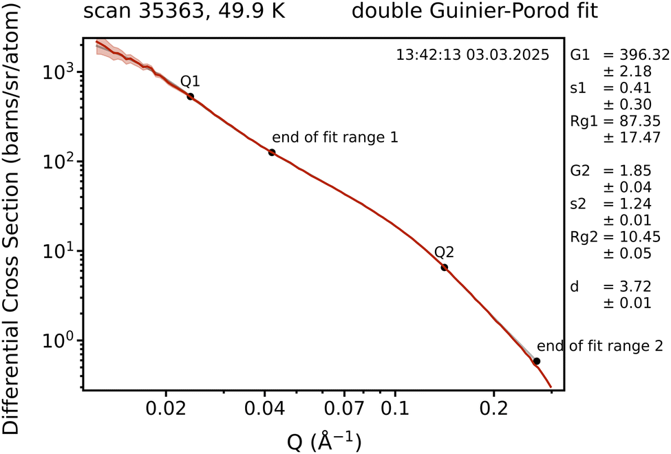Fig. 2 Fitting of GP model to a DCS as a function of Q plot of a sample deposited at 50 K. GP model in grey and data in red.

Both the Porod and GP model fittings were done using Python codes.⁴⁵

One limitation of the Guinier–Porod model is that it uses arbitrary scaling factors that cannot be (easily) linked to the overall volume of scattering centres – porosity in this case. Using SASView, a program for the analysis of small angle scattering data, we applied a shape-based lamellar pore model to calculate porosity.⁴⁶ This model assumes lamellar pores and was chosen as the SANS curve slope indicates the presence of lamellar dominated shapes as it follows a Q⁻² dependence at the lowest Q section. We created a customized version of the model by summing SASView's inbuilt lamellar pore model and its inbuilt Gaussian model to obtain:

where the lamellar scale factor P represents the porosity (pore volume divided by total sample volume – i.e. the volume fraction the pores occupy in the whole sample volume), δ is the bilayer thickness (pore width) when assuming randomly oriented lamellae (pores), and the Gaussian peak scale factor S reflects the distance between pores as mean spacing of the lamellae, w = 2π/Q₀. Additionally, we applied polydispersity when fitting with the distribution looking rather broad.

3.2 Full Q range data analysis

SANS measures an inverse transform of the scattering centre size distribution in real space. Obtaining a size distribution through this inverse transform is not possible without ideal counting statistics and a complete range of all the scattering vectors Q. Additionally, it is complicated by the fact that the measured intensity profile can be made up by many different arrangements of scattering centre size and volume fraction.⁴⁷

To interpret the measured cross-section over the fully measured Q-range for each merged ASW sample data set, we used the computer routine MAXE. MAXE uses the maximum entropy algorithm to perform the inverse transform of the SANS intensity to yield a pore size distribution (assuming spherical pores).^47–49 It does so by fitting the most featureless and disordered distribution (highest entropy) that it can to the data through an iterative procedure that accounts for the chi-squared statistic. The advantage of MAXE is that it avoids the need to assume any prior model of the size distribution of inhomogeneous scatterers (pores in this case), and it covers the full measured Q-range, rather than the limited range used in the GP, Lamellar and Porod models.

Using spheres is of course a simplification, but it does allow us to consistently assess changes in observed pore size distribution as a function of deposition temperature, by reproducing the neutron data. Our aim was to exploit a number of different analysis methods to model our ice behaviour. Each model has different assumptions around the ice structure, independent of the other analysis methods, and this tests whether disparate analyses can generate similar results, as ASW porosity is likely too complex to be fully described by a simple model.

MAXE yields the fractional volume distribution C(D), where C(D)δD gives the volume fraction V(D) of pores with diameters comprised in [D, D + δD], normalised over the total pore volume. When using the software, we accounted for the accessible Sans2d length scale range by setting the pore size range as 0 to 4000 Å, with a bin size of 2 Å. These parameters were chosen as they best describe the pore size distribution. For example, reducing the fitting range and/or number of bins leads to a bad description of the first peak and generates artifacts at a high pore diameter.

From the pore size distribution, the total pore volume fraction V_pores, representing a direct measure of the material porosity, defined as the occupied volume over the total volume, can be derived:

Similarly, the total pore surfaces S_pores is extracted from the distribution using:

This gives a direct measure of the specific surface area, usually obtained from the Porod model for the pure NIMROD data. Uncertainties of both the total pore volumes and specific surface areas were estimated by summing the relative uncertainties from background calculations, sample thicknesses and sensitivity on binning.

4 Results

4.1 NIMROD

4.1.1 DCS curves. As discussed previously, the output of reducing NIMROD data is the DCS as a function of Q. Prior to any analysis, there is already information about the ice presented in this original processed data.

Fig. 3 shows an example plot of the DCS as a function of Q for a sample deposited at 40 K. The low Q slope on the left hand side of this plot (the SANS region) is scattering due to surface (Porod) scattering from grain surfaces, while the ‘hump’ that is superimposed on this slope at ∼0.1 Å⁻¹ is due to the porosity of the ice. In the high Q region, there is information on the local structure. Sharp Bragg peaks would show crystalline structure, whereas smooth diffuse scattering, as seen in Fig. 3 at ∼2 Å⁻¹, indicates amorphous ice structure.

Fig. 3 Differential cross section as an function of Q for a sample deposited at 40 K. The left side of the plot is the SANS region, wherein the slope is created by the granularity of the ice and the right side of the plot, the diffraction region, shows how amorphous the ice is.

This DCS as a function of Q plot for all the samples is shown in Fig. 4. With increasing deposition temperature, the low Q hump flattens, indicating less porosity in the samples deposited at higher temperatures. As shown in the enlarged view of the high Q portion of the plot, there are increasingly cubic crystalline diffraction patterns observed (Bragg peaks forming), meaning the ice is more crystalline at higher deposition temperatures. What is very advantageous of this neutron scattering method is that all of this information is obtained simultaneously – that the ice is both porous and amorphous. Even when growing an ice at higher temperatures, we still observe granularity.

Fig. 4 DCS as a function of Q for each sample. Trace colours represent the respective temperatures, as shown by the colourbar on the right hand side. The inset shows the high Q region enlarged.

Another advantage of neutron scattering is that there is already a scattering signal with all the salient features of the structure observed after depositing for 15 minutes (a film with thickness of approx. 0.002 cm of ice, estimated from the absolute scattering level at high Q), although with less than desirable statistics. We however still grow the ice for 12 hours in order to get good statistics and a better signal-to-noise ratio. Fig. 5 shows this evolution of the DCS as a function Q plot with time for the ice samples of deposition temperatures 30, 80 and 120 K. Throughout the deposition, both the SANS and high Q region increase in intensity, while the signal-to-noise ratio improves at highest Q. Although there is the finesse of taking data every 15 minutes, the scans are averaged to hours in order to get better statistics.

Fig. 5 DCS as a function of Q plots for every hour of the ice samples deposited at 30 (left panel), 80 (middle panel) and 120 K (right panel). Within each panel, the high Q region is enlarged to better show crystallinity. Trace colours represent the time elapsed during deposition from blue to yellow.

4.1.2 Model fitting results. We chose a range of fitting methods with differing balance in terms of number of prior assumptions and richness of the resulting data, noting that all give a similar picture of the changes in ASW porous structure.

The minimum Q of NIMROD is ≈0.015 Å⁻¹ and the maximum length scales are limited to being on the order of 2/Q. Due to this, NIMROD cannot access certain larger features, meaning that when, for example, porosity is discussed, it is nano-porosity that is being referred to.

Fig. 6 shows the ice thickness, estimated from the total scattering level at high Q, as a function of deposition time for each sample. The figure shows that, as the ices are grown, there is a consistent increase in ice thickness throughout the deposition. Across all the samples, the rate of thickness increase is very similar. However, the thickness values at the end of deposition differ, where samples deposited at higher temperatures finish with lower thicknesses.

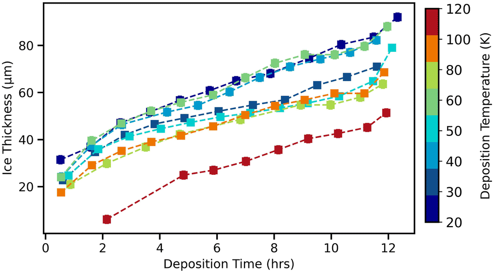Fig. 6 Ice thickness as a function of time from NIMROD data. This is estimated from the scattering levels in the high Q region whereby we keep the packing fraction fixed and assume that the D₂O sample density is 1.04 g cm⁻³.² Trace colours represent the deposition temperature of the sample, represented by the colourbar on the right hand side.

The change in ice thickness obtained in this work across the deposition temperatures is much larger than that found by the experimental work of Bossa et al. (2012) who observed a 13% decrease in ice height from deposition temperatures of 20 to 120 K.¹² This could likely be due to differences in the samples grown. The samples herein are much thicker than other experimental works and so can have larger pore networks at low temperature that are not present at high deposition temperatures, creating more drastic differences between samples. However, our observation that ASW vapour-deposited at temperatures below 130 K is amorphous and porous is commensurate with the wider literature.^{3,11,14,16,27,50,51} This furthers the argument made by Scott Smith et al. (2009) that the incident particles must truly hit and stick, or at least have limited mobility, or else particle mobility/diffusion would likely act to fill the voids regions, thereby reducing porosity.⁵²

Fig. 7 shows that, with increasing deposition temperature, the porosity and surface area (SSA) decrease. There is a clear linear correlation between SSA and deposition temperature, with SSA decreasing with the latter. However, it is important to note that this SSA decrease is also accompanied by a decrease in the height of the ice with deposition temperature (as seen in Fig. 6) as the pore populations (types, shapes and sizes) are different.

Fig. 7 Specific surface area (left y axis and data points in black) and porosity (right y axis and data points in orange) as a function of deposition temperature. The porosity values are calculated by fitting the Lamellar pore model to the NIMROD data and the SSAs obtained through fitting the Porod model.

For porosity, the picture is more complex and has much larger relative errors to the values measured (error bars are plotted but invisible for SSA data) because of this uncertainty in the ice height. Fundamentally, the number of molecules in the neutron beam and on the ice surface remains constant, but the volume occupied by the ice decreases – the SSA decreases and the porosity varies.

The porosity, as this paper shows and will continue to discuss later on, is a combination of two populations of pores. For the samples deposited at lower temperatures (below 80 K), this pore volume for porosity is dominated by nanopores. The pore volume for the samples deposited at temperatures above 80 K is dominated by larger scale pores (later in the paper we distinguish these by referring to them as ‘voids’ but for now retain the nomenclature ‘pore’). Therefore, the 80 K deposition is a (somewhat arbitrary) turning point – clearly this may not be at exactly 80 K but appears around this value in our data set. This hypothesis is corroborated later by our MAXE analysis of the pore size distribution (see Fig. 11), where it can be clearly seen that the 80 K ice is the first to not include the smallest pore sizes, and where the larger pores start to form in the ice. It is also the first temperature point where the total pore volume is not dominated by the smallest ice pores.

Other similar experimental studies typically find a general linear decrease in porosity with increasing deposition temperature, whereas the porosity calculated in this work shows this more complex trend with deposition temperature. Most other studies find a complete lack of porosity at higher deposition temperatures.^3,14,16 For example, Stevenson et al. (1999) observed almost no N₂ adsorption for deposition temperatures of 90 K onwards; Kimmel et al. (2001) found that ASW films grown above 90 K had essentially the same N₂ adsorption capacity as their crystalline reference ice at 140 K; Mate et al. (2012) found no sign of any dangling OH bonds (proxy for porosity) for ices grown at 90 K; and Clements et al. (2018) state that at 130 K, their ice structures are completely smooth with no porosity.^9,11,14,27 These findings differ to this work's as the 120 K sample still has significant porosity, even though the ice itself seems relatively compact (based on its thickness, seen in Fig. 6). There are however thickness differences between this work and that of Stevenson et al. (1999) and Kimmel et al. (2001) who work with thin films, which must be kept in mind when comparing. Additionally, some other studies are only capable of probing open pores and not closed pores as well.

4.1.3 Nanoporosity. Analysis of the double Guinier–Porod (GP) model fits allow additional insight into the SSA and porosity results. Although two sets of GP parameters are obtained due to the two structural features observed in the low Q slope, only those of the second GP fitting will be presented here. This second GP fitting probes smaller length scales than the first (fits Q range 0.065–0.25 Å⁻¹), meaning that it fits over the nanoporosity ‘hump’ of the slope, that was discussed previously. This section focusses on the nanoporosity and so only the NIMROD data is needed. The first GP fitting of the NIMROD data that covers the large scale set of pores pushes the limit of what NIMROD can probe and therefore obtains large uncertainties. Due to this, those results will be omitted from this section as the following section will instead present the full porosity results obtained from the combined SANS data.

Fig. 8 shows that the radius of gyration values at the end of deposition with increasing deposition temperature for the smallest pore populations in each sample. At first glance these appear to simply increase linearly (apart from the sample deposited at 80 K) – meaning an increase in pore diameter. However, as discussed with relation to Fig. 7, we see again evidence for two pore populations in the radius of gyration data in Fig. 8. In this scenario, consider that the 80 K data point is a point of inflection (not an anomalous point) where the crossover between the ice structure being dominated by nanopores and being dominated by larger pores occurs. This is why we have not tried to fit ‘straight’ lines to Fig. 7 and 8 (radius of gyration and s parameter). In both cases, the smallest pores whose properties are extracted from the GP fit are not actually the same populations – one set for ices deposited below 80 K are nanopore dominated and the other dominated by larger pores between the ice grains (later called ‘voids’). The fact that Fig. 7, 8 and 11 are all generated by different methods of analysis of the data, but show the same picture of a ‘crossover’ point at 80 K reassures us that this hypothesis with respect to pore types and volumes is strongly corroborated by the experimental evidence.

Fig. 8 The final Guinier–Porod parameter values (at the end of ice growth) as a function of deposition temperature. This is for the second set of GP values, that represents the smaller population of pores.

Based on the s parameter, shown in the middle panel of Fig. 8, the nanopores transition from a 2D lamellar ‘flattened’ dominated shape to a more spherical shape. In addition to this, the surface becomes increasingly rough with increasing deposition temperature, based on the d parameter. The GP values as a function of deposition time are shown in Fig. S1 in the ESI.†

From fitting the Lamellar pore model, a pore width is obtained and Fig. 9 shows the comparison of this porewidth with R_g. With the Lamellar pore model, there is little change between deposition temperatures of 20 and 100 K. The sample deposited at 120 K however displays a final pore width that is 7 orders of magnitude larger than the other samples. At the lower temperatures, the Lamellar pore model obtains pore widths that are similar to the nanoporosity radius of gyration values from the GP model. For the 120 K sample, the Lamellar pore model then has a value that is in the realm of the larger population of pores.

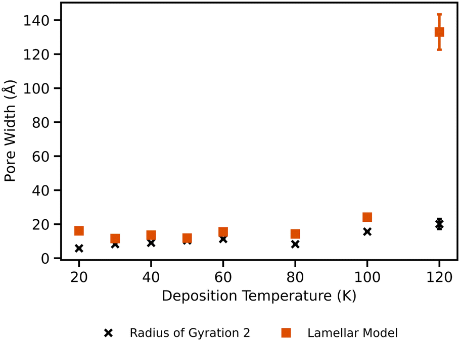Fig. 9 Comparison of the radius of gyration values from the GP model and the pore widths obtained from the Lamellar pore model, as a function of deposition temperature. These values are the widths at the end of the ice growth.

Overall, the 120 K sample shows significantly different features than that of the 100 K sample, whereby its surface is much smoother (based on d parameter from GP fitting) and it has much larger pore widths. This difference can be attributed to the onset of the glass transition of water, allowing for increased water mobility and subsequent structural relaxation.⁴ Hill et al. (2016) found that at 115 K, cooperative and non-translational motion of water sets in, with the transition completing at about 136 K.⁵³ As this 120 K sample was deposited so near to this threshold, it is unsurprising that it exhibits very different behaviour to the other samples. The smoother interface of our 120 K sample is similar to the simulation results of Clements et al. (2018) who obtained smoother ices at higher deposition temperatures as well.

4.2 Combined SANS

The results obtained from NIMROD form a solid foundation of understanding how deposition temperature affects the structural nanoporosity of ASW. However, as previously discussed, the size of the larger pores observed pushed beyond what NIMROD could probe with good accuracy, and this is why we used Sans2d. The NIMROD data is still invaluable as it ensures consistency, that the ice is ASW (from high Q region) and it allows estimates of sample thickness used for normalisation when reducing Sans2d data.

Fig. 10 shows the intensity as a function of Q for the final deposition hour of each sample (raw Sans2d data). All of the samples, aside from the sample deposited at 120 K, have a very similar shape with good overlap and feature a prominent shoulder at around 10⁻¹ Å⁻¹. The sample deposited at 120 K has a shoulder at much lower Q – around 0.4 Å⁻¹. These curves as a function of deposition time for each sample are shown in Fig. S2 in the ESI.†

Fig. 10 Intensity as a function of Q for the final deposition hour of each sample. Trace colours represent the deposition temperature of the sample, shown by the colourbar on the right hand side.

4.2.1 Full porosity. The MAXE software was used on the merged data (shown in Fig. S3 in the ESI†) to obtain a pore size distribution for each sample. Fig. 11 shows the obtained pore size distributions at the end of deposition of each sample. Samples deposited at lower temperature have pores that overall take up a larger volume fraction of the ice than those deposited at higher temperatures. It is seen clearly that there is in fact a bimodal nature to the pore size distribution, rather than unimodal. At low deposition temperatures, the two pore populations are of sizes ∼10 Å and ∼85 Å, which become larger with increasing deposition temperature. For the sample deposited at 120 K, the population sizes are at ∼60 Å and ∼400 Å, and it has a very small volume fraction for both populations compared to the other samples. Overall, samples deposited at higher temperatures therefore have larger pore sizes than those deposited at lower temperatures and the second larger population of pores is an order of magnitude larger than those of the lower deposition temperature samples.

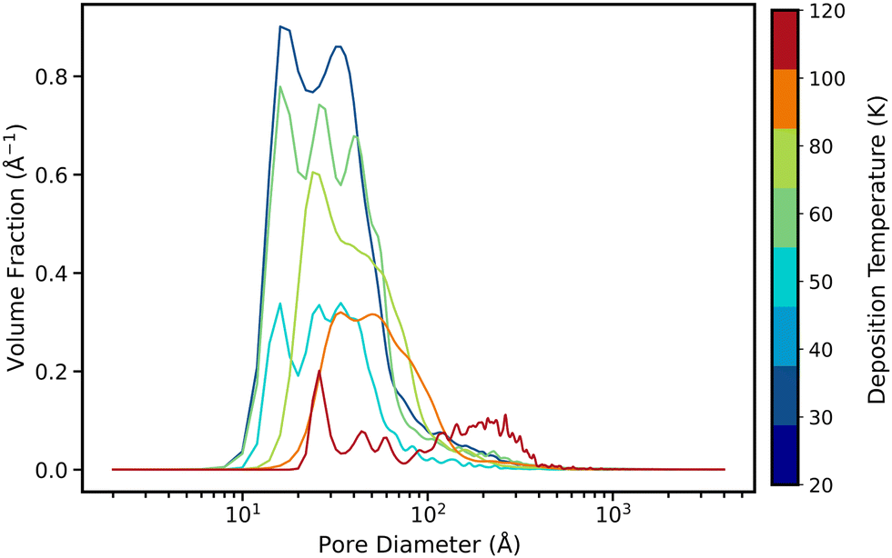Fig. 11 Volume fraction as a function of pore diameter for each sample. Trace colours represent the deposition temperature, shown by the colourbar on the right hand side.

Although NIMROD hinted at there being two distinct populations of pores (based on the GP fittings), the analysis of the merged SANS data confirms this. Having two populations of pores within our work is similar to what was found in the laboratory experiments of Carmack et al. (2023) who obtained mostly microporous samples that likely had larger mesopores present, based on their desorption kinetics.⁴³ In the work of Raut et al. (2008), the presence of both micro and mesopores has also been used to explain the dangling bond destruction rate observed in background-deposited ASW samples.⁵⁴

The total pore volumes obtained from the merged NIMROD and Sans2d data are a bit higher than those calculated for the pure NIMROD data, as a consequence of the extended Q-range, allowing a more extended view on all pore sizes. This is particularly important at high temperatures where the strongest contribution to porosity comes from larger pores, which are outside of NIMROD's range. Additionally, the methods of calculating porosity are different for each data set; however, this does strengthen the reliability of the porosity range as the two methods get similar results.

Fig. 12 and 13 show the comparison of porosity and SSA for each sample as a function of deposition time. For both porosity and SSA, there is a steady and small increase over deposition time for every sample. The samples deposited at lower temperatures have higher porosity and SSA than those deposited at higher temperatures, with the 120 K displaying especially low surface area values.

Fig. 12 Porosity as a function of deposition time for every sample, with trace colours representing the deposition temperature of the sample, shown by the colourbar on the right hand side.

Fig. 13 Specific surface area as a function of deposition time for every sample, with trace colours representing the deposition temperature of the sample, shown by the colourbar on the right hand side.

5 Discussion

Within the literature, there has been much speculation over the overall ASW pore structure. Stevenson et al. (1999) and Kimmel et al. (2001) refer to ASW as having a homogeneous, “sponge-like” structure, where most of the pores are accessible to adsorbates.^14,27 Additionally, the Monte Carlo studies of Cuppen et al. (2007) and Garrod (2013) get “skyscraper”- and cauliflower-like structures (ice towers separated by randomly oriented pores), respectively.^21,55 As previously mentioned, Carmack et al. (2023) hinted at there being actually two populations of pores within background deposited ASW: micro and mesopores.⁴³ They concluded this by comparing their DB2′ (shift of dangling bond absorption band 3696 to 3669 cm⁻¹ after CH₄ attachment) growth rate with CH₄ uptake to that of the work of Raut et al. (2007), as there was not only the presence of micropores, but also the likely presence of larger mesopores in their own work.¹³ These mesopores allowed for multilayer adsorption within the pore space.

Another spectroscopy study adding to this is that of Rosu-Finsen et al. (2016) who grew ballistically deposited ASW on an amorphous SiO₂ surface at 17 K.⁵⁶ They measured the time evolution of the RAIR spectra in the region of the O–H stretching vibrations (vOH), and observed an increase in the vOH band intensity and associated it with agglomeration of isolated H₂O and small H₂O clusters into larger ASW islands, at temperatures below 25 K. For temperatures above 25 K, both agglomeration and hydrogen bond network formation are reported as being able to occur in parallel. They conclude that this has an important impact on chemistry as H₂O will not accrete as a uniform thin film on a surface, but rather as three-dimensional islands with exposed surface. Further to this, Scott Smith et al. (1996) and Marchione et al. (2019) see these islands through their ASW desorption studies.^57,58 Zero-order kinetics are expected if sublimation were to occur from a smooth film of constant exposed area; however, Scott Smith et al. (1996) find that the ASW desorption kinetics are not consistent with zero-order evaporation. Marchione et al. (2019) then state that their desorption kinetics, associated with multilayer desorption, indicate that the H₂O molecules must be in clusters or islands on the surface before or during desorption. Therefore, they must either grow as islands or agglomerate to form clusters or islands prior to desorption.

This paper provides direct experimental evidence of these two populations of pores that have been under debate. Our ASW structures seemingly grow in islands/grains with voids between them and so porosity is thus a combination of the void volume and the volume of the nanopores in the islands themselves (illustrated in Fig. 14). This conclusion is obtained from the two structural features observed in the SANS region of the DCS as a function of Q (see Fig. 3, 5 and 4) – representing the two populations of pores with differing scales.

Fig. 14 Cartoon representation of the structure of ASW theorised in this work – islands/grains with voids between them (not to scale). ASW deposited at the lowest temperatures (20 K in this case shown on the left) features islands with nanopores within them, whereas ASW deposited at the highest temperatures (120 K in this case on the right) feature larger compact grains separated by much larger voids. Length scales of each are stated within each label.

The islands/grains + voids structure we observe is likely most similar to the Monte Carlo structures of Garrod (2013).²¹ These structures are cauliflower-like with irregularity on all scales and significant uniform porosity. Some of their pores/crevices pass deep within the mantle, almost down to the dust grain itself. The smallest florets of the ice structures herein are ice towers of around 100 Å in diameter separated by randomly oriented lamellar pores of around 15 Å width at the lowest temperature.

Using the double GP model on the NIMROD data illuminated the presence of two populations of pores by extracting two radius-of-gyration data sets. The nanopores follow the trend found in the literature, wherein increasing deposition temperatures obtained less or none of the nanopores. For the voids, the opposite is true as they come to dominate at higher deposition temperatures, shown by the drastic increase in porewidth for the 120 K sample from the Lamellar pore model analysis. However, the NIMROD results related to the larger population of pores had large uncertainties and therefore the combined NIMROD + Sans2d data has now confirmed the results, but with greater accuracy. It is seen in the full low-Q data analysis results that the two population of pores are present at the lowest deposition temperatures (below 80 K); however, samples deposited at higher temperatures likely have compact islands with larger voids between them.

6 Conclusions

We have used total neutron scattering and SANS to investigate how deposition temperature impacts the structure of vapour-deposited ASW. From this, we have provided further direct experimental evidence that deposition temperature does have a significant effect on the ASW structure. With increasing deposition temperature, the ASW structure becomes more akin with a compact ice, whereby there is less surface area and a change in porosity – in line with the results of other works.^{3,10,14,16,27,29} What this work adds to the wider literature is a direct way of probing the ASW structure and direct experimental evidence of the presence of two populations of pores.

Our main findings are the following:

1. Porosity is retained throughout the growth and differs depending on the deposition temperature, whereby size and shape of pores change – consistent with wider literature. How the porosity changes in turn affects the surface area.

2. There are likely two populations of pores which change differently with deposition temperature.

3. Even at higher deposition temperatures, a fully compacted ice is not grown, there is still granularity and porosity present from the void volume.

It must be kept in mind however, when comparing to other thin film studies, that we grow thicker ices, as this is needed for neutron scattering studies. Nevertheless, it is important that the above findings are incorporated when attempting to model or interpret chemical reactions occurring on ASW, or to simply understand the ASW structure itself.

Author contributions

Z. Amato: formal analysis, investigation, software, visualization, writing – original draft and writing – review & editing. T. F. Headen and H. J. Fraser: conceptualization, funding acquisition, investigation, methodology, project administration, resources, supervision, validation and writing – review & editing. S. Gärtner: conceptualization, investigation, methodology, software and validation. P. Ghesquière: formal analysis, investigation, methodology and software. T. Youngs, D. Bowron, L. Cavalcanti, S. Rogers: investigation, methodology, resources and software. N. Pascual, O. Auriacombe, E. Daly, R. E. Hamp, R. K. TP: investigation. C. R. Hill: investigation, methodology and software.

Data availability

Data for this article are available at ref. 59, 60 and 61. The data analysis scripts are found at ref. 45.

Conflicts of interest

There are no conflicts to declare.

Acknowledgements

Astrochemistry at the Open University is currently supported by STFC under grant agreement numbers ST/X001164/1, ST/T005424/1 and ST/Z510087/1 and Z. Amato also thanks The Open University for funding his PhD studentship in part. Earlier research leading to the original experimental work presented in this paper was undertaken at the OU and previously supported by UK Space Agency, EU COST Action CM1401 and UKRI – STFC under grant agreement numbers ST/M003051/1 and ST/P000584/1. We thank the STFC ISIS Neutron and Muon Source for award of beamtime allocations RB1510246⁵⁹ and RB1610318⁶⁰ on NIMROD and RB2010205⁶¹ on Sans2D, and for partly funding Z. Amato through the ‘ISIS Facilities Development Studentship’ scheme. We would like to acknowledge and thank the ‘Pressure and Furnace’, ‘Cryogenics’, ‘Electronics’ and ‘Soft Matter’ groups at the ISIS Neutron and Muon Source as their setting up/maintaining of the dedicated deposition setup is vital to our work. We especially thank Chris Goodway for his help in the design and construction of the deposition setup. This work benefited from the use of the SasView application, originally developed under NSF award DMR-0520547. SasView contains code developed with funding from the European Union's Horizon 2020 research and innovation programme under the SINE2020 project, grant agreement no 654000.

References

1. J. L. Abascal and C. Vega, J. Chem. Phys., 2005, 123, 234505.
2. D. T. Bowron, J. L. Finney, A. Hallbrucker, I. Kohl, T. Loerting, E. Mayer and A. K. Soper, J. Chem. Phys., 2006, 125, 194502.
3. D. E. Brown, S. M. George, C. Huang, E. K. L. Wong, K. B. Rider, R. S. Smith and B. D. Kay, J. Phys. Chem., 1996, 100, 4988–4995.
4. J. P. Devlin, J. Geophys. Res.: Planets, 2001, 106, 33333–33349.
5. A. Al-Halabi, H. J. Fraser, G. J. Kroes and E. F. V. Dishoeck, Astron. Astrophys., 2004, 422, 777–791.
6. P. Ehrenfreund, H. J. Fraser, J. Blum, J. H. Cartwright, J. M. Garcia-Ruiz, E. Hadamcik, A. C. Levasseur-Regourd, S. Price, F. Prodi and A. Sarkissian, Planet. Space Sci., 2003, 51, 473–494.
7. R. S. Smith, C. Huang, E. K. L. Wong and B. D. Kay, Phys. Rev. Lett., 1997, 79, 909–912.
8. S. Malyk, G. Kumi, H. Reisler and C. Wittig, J. Phys. Chem. A, 2007, 111, 13365–13370.
9. B. Mate, Y. Rodriguez-Lazcano and V. J. Herrero, Phys. Chem. Chem. Phys., 2012, 14, 10595–10602.
10. D. J. Burke and W. A. Brown, Phys. Chem. Chem. Phys., 2010, 12, 5947–5969.
11. A. R. Clements, B. Berk, I. R. Cooke and R. T. Garrod, Phys. Chem. Chem. Phys., 2018, 20, 5553–5568.
12. J. B. Bossa, K. Isokoski, M. S. D. Valois and H. Linnartz, Astron. Astrophys., 2012, 545, A82.
13. U. Raut, M. Fama, B. D. Teolis and R. A. Baragiola, J. Chem. Phys., 2007, 127(20), 204713.
14. K. P. Stevenson, G. A. Kimmel, Z. Dohnalek, R. S. Smith and B. D. Kay, Science, 1999, 283, 1505–1507.
15. N. Watanabe and A. Kouchi, Prog. Surf. Sci., 2008, 83, 439–489.
16. N. Horimoto, H. S. Kato and M. Kawai, J. Chem. Phys., 2002, 116, 4375–4378.
17. H. Li, A. Karina, M. Ladd-Parada, A. Spah, F. Perakis, C. Benmore and K. Amann-Winkel, J. Phys. Chem. B, 2021, 125, 13320–13328.
18. C. Mitterdorfer, M. Bauer, T. G. Youngs, D. T. Bowron, C. R. Hill, H. J. Fraser, J. L. Finney and T. Loerting, Phys. Chem. Chem. Phys., 2014, 16, 16013–16020.
19. O. Galvez, B. Mate, V. J. Herrero and R. Escribano, Icarus, 2008, 197, 599–605.
20. M. P. Collings, M. A. Anderson, R. Chen, J. W. Dever, S. Viti, D. A. Williams and M. R. McCoustra, Mon. Not. R. Astron. Soc., 2004, 354, 1133–1140.
21. R. T. Garrod, Astrophys. J., 2013, 778, 158.
22. T. Hama, K. Kuwahata, N. Watanabe, A. Kouchi, Y. Kimura, T. Chigai and V. Pirronello, Astrophys. J., 2012, 757, 185.
23. R. A. Baragiola, Planet. Space Sci., 2003, 51, 953–961.
24. D. Laufer, E. Kochavi and A. Bar-Nun, Phys. Rev. B: Condens. Matter Mater. Phys., 1987, 36, 9219–9227.
25. J. B. Bossa, K. Isokoski, D. M. Paardekooper, M. Bonnin, E. P. V. D. Linden, T. Triemstra, S. Cazaux, A. Tielens and H. Linnartz, Astron. Astrophys., 2014, 561, A136.
26. A. Bar-nun, G. Herman, D. Laufer and M. L. Rappaport, Icarus, 1985, 63, 317–332.
27. G. A. Kimmel, Z. Dohnalek, K. P. Stevenson, R. S. Smith and B. D. Kay, J. Chem. Phys., 2001, 114, 5295–5303.
28. Z. Dohnalek, G. A. Kimmel, P. Ayotte, R. S. Smith and B. D. Kay, J. Chem. Phys., 2003, 118, 364–372.
29. E. Vichnevetski, P. Cloutier and L. Sanche, J. Chem. Phys., 1999, 110, 8112–8118.
30. D. T. Bowron, A. K. Soper, K. Jones, S. Ansell, S. Birch, J. Norris, L. Perrott, D. Riedel, N. J. Rhodes, S. R. Wakefield, A. Botti, M. A. Ricci, F. Grazzi and M. Zoppi, Rev. Sci. Instrum., 2010, 81, 033905.
31. R. K. Heenan, S. E. Rogers, D. Turner, A. E. Terry, J. Treadgold and S. M. King, Neutron News, 2011, 22, 19–21.
32. A. Soper, Gudrun Software, 2024, https://www.isis.stfc.ac.uk/Pages/Gudrun.aspx, Accessed: 2024-06-25.
33. Mantid, Software, 2024, https://www.mantidproject.org/, Accessed: 2024-06-25.
34. O. Arnold, J. Bilheux, J. Borreguero, A. Buts, S. Campbell, L. Chapon, M. Doucet, N. Draper, R. Ferraz Leal, M. Gigg, V. Lynch, A. Markvardsen, D. Mikkelson, R. Mikkelson, R. Miller, K. Palmen, P. Parker, G. Passos, T. Perring, P. Peterson, S. Ren, M. Reuter, A. Savici, J. Taylor, R. Taylor, R. Tolchenov, W. Zhou and J. Zikovsky, Nucl. Instrum. Methods Phys. Res., Sect. A, 2014, 764, 156–166.
35. B. Hammouda, Probing Nanoscale Structures – the SANS toolbox, 2008, https://api.semanticscholar.org/CorpusID:139951325.
36. T. J. Su, J. R. Lu, Z. F. Cui, R. K. Thomas and R. K. Heenan, Langmuir, 1998, 14, 5517–5520.
37. R. Strey, J. Winkler and L. Magid, J. Phys. Chem., 1991, 95, 7502–7507.
38. L. Feigin and D. Svergun, Structure Analysis by Small-Angle X-Ray and Neutron Scattering, Springer, US, Boston, MA, 1987.
39. NIST, Neutron activation and scattering calculator, https://www.ncnr.nist.gov/resources/activation/, 2025, Accessed: 2025-01-14.
40. T. Loerting, I. Kohl, W. Schustereder, K. Winkel and E. Mayer, ChemPhysChem, 2006, 7, 1203–1206.
41. A. H. Narten, C. G. Venkatesh and S. A. Rice, J. Chem. Phys., 1976, 64, 1106–1121.
42. J. A. Ghormley and C. J. Hochanadel, Science, 1971, 171, 62–64.
43. R. A. Carmack, P. D. Tribbett and M. J. Loeffler, Astrophys. J., 2022, 942, 1.
44. B. Hammouda, J. Appl. Crystallogr., 2010, 43, 716–719.
45. Z. Amato, Batch Analysis ASW, 2025, https://github.com/ZacAmato/Batch_Analysis_ASW, Accessed: 2025-01-03.
46. SasView, Software, 2024, https://www.sasview.org/, Accessed: 2024-06-25.
47. H. Jazaeri, P. J. Bouchard, M. T. Hutchings, A. A. Mamun and R. K. Heenan, Mater. Sci. Technol., 2015, 31, 535–539.
48. J. A. Potton, G. J. Daniell and B. D. Rainford, J. Appl. Crystallogr., 1988, 21, 891–897.
49. P. R. Jemian, MAXE Software, 2024, https://github.com/prjemian/sizes, Accessed: 2024-06-25.
50. U. Essmann and A. Geiger, J. Chem. Phys., 1995, 103, 4678–4692.
51. J. He, A. R. Clements, S. M. Emtiaz, F. Toriello, R. T. Garrod and G. Vidali, Astrophys. J., 2019, 878, 94.
52. R. S. Smith, T. Zubkov, Z. Dohnalek and B. D. Kay, J. Phys. Chem. B, 2009, 113, 4000–4007.
53. C. R. Hill, C. Mitterdorfer, T. G. Youngs, D. T. Bowron, H. J. Fraser and T. Loerting, Phys. Rev. Lett., 2016, 116, 215501.
54. U. Raut, M. Fama, M. J. Loeffler and R. A. Baragiola, Astrophys. J., 2008, 687, 1070.
55. H. M. Cuppen and E. Herbst, Astrophys. J., 2007, 668, 294.
56. A. Rosu-Finsen, D. Marchione, T. L. Salter, J. W. Stubbing, W. A. Brown and M. R. S. McCoustra, Phys. Chem. Chem. Phys., 2016, 18, 31930–31935.
57. R. S. Smith, C. Huang, E. K. L. Wong and B. D. Kay, Surf. Sci., 1996, 367, L13–L18.
58. D. Marchione, A. Rosu-Finsen, S. Taj, J. Lasne, A. G. M. Abdulgalil, J. D. Thrower, V. L. Frankland, M. P. Collings and M. R. McCoustra, ACS Earth Space Chem., 2019, 3, 1915–1931.
59. H. J. Fraser, Understanding Structural Changes in Amorphous Solid Water (ASW) on Heating, 2015 DOI:10.5286/ISIS.E.RB1510246.
60. H. J. Fraser, What really governs porosity in Amorphous Solid Water (ASW)? 2016 DOI:10.5286/ISIS.E.RB1610318.
61. P. Ghesquière, Evolution of porosity and structure of Amorphous Solid Water (ASW), 2022 DOI:10.5286/ISIS.E.RB2010205.

---

Footnote

† Electronic supplementary information (ESI) available. See DOI: https://doi.org/10.1039/d5cp00270b

---