
 Open Access Article
 This Open Access Article is licensed under a
 Creative Commons Attribution 3.0 Unported Licence
A general, robust framework for determining the key species that forewarns sudden transitions in biological circuits†
Dinesh
Kashyap
 a,
Taranjot
Kaur
b,
Partha Sharathi
Dutta
b and
Sudipta Kumar
Sinha
*a
a,
Taranjot
Kaur
b,
Partha Sharathi
Dutta
b and
Sudipta Kumar
Sinha
*a
aTheoretical and Computational Biophysical Chemistry Group, Department of Chemistry, Indian Institute of Technology Ropar, Rupnagar–140001, India. E-mail: sudipta@iitrpr.ac.in
bDepartment of Mathematics, Indian Institute of Technology Ropar, Rupnagar–140001, India. E-mail: parthasharathi@iitrpr.ac.in
First published on 22nd April 2025
Abstract
The Cdc2-cyclin B/Wee1 kinase system exhibits bistability between alternative steady states, which emerges due to the mutual inhibition between Cdc2-cyclin B and Wee1 kinases. Alternative steady states are the M phase-like state and G2 arrest state, which have implications in cell cycle progression at the G2 phase in eukaryotic cells. A slight alteration in the feedback strength can drive sudden transitions between these contrasting alternative states upon crossing a critical threshold or a tipping point. The phenomenon of critical slowing down (CSD) has been widely used to identify the proximity to a tipping point. However, determining the key variable or species that best signals CSD is a challenging task and holds significance in complex biochemical processes. Here, we determine the key variable or observation direction (OD) from the direction of CSD to best detect an upcoming transition in the Cdc2-cyclin B/Wee1 model system. We find that with increasing feedback strength, the Cdc2-cyclin B is the OD, as it produces a stronger signal than that of Wee1. With decreasing feedback strength, both Cdc2-cyclin B and Wee1 produce similar signals and can be used as the OD. Furthermore, the noise-sensitive direction highlights the effect of stochasticity in Cdc2-cyclin B and Wee1 for increasing and decreasing feedback strength, respectively. We also perform sensitivity analyses that reveal the robustness of the OD. Finally, we compare the efficacy of OD with principal component analysis while detecting a tipping point, and also validate its general applicability to epithelial–mesenchymal transition for cancer progression.
1 Introduction
Critical transitions refer to an abrupt shift in the state of a dynamical system upon crossing a tipping point due to small changes in the driver parameter and are observed in numerous multistable nonlinear systems, ranging from molecular biology to large-scale ecology. The tipping point refers to a critical threshold on surpassing which an abrupt shift occurs.1–4 Commonly, a tipping point corresponds to a saddle-node bifurcation point (where one stable equilibrium point and one unstable equilibrium point collide and disappear), as the system undergoes a qualitative change in its steady-state behavior with variations in the system parameter. For instance, a sudden transition from the epithelial to the mesenchymal (EMT) state in cells,3 from insulin sensitive to insulin-resistant state in human bodies,5 from grassland to woodland in the forest Savanna,6etc. are a few practical examples of critical transitions. Forewarning such critical transitions in biological systems is of paramount importance as the sudden change from one stable state to another is often undesirable, e.g., sudden shifts from a healthy physiological state to the onset of diseases such as cancer,7 depression,8 and gut microbiome dysregulation.9 A key characteristic in predicting these transitions is the phenomenon of critical slowing down (CSD). CSD occurs when the system experiences slower recovery from perturbations in the proximity of the tipping point. Furthermore, prior to a critical transition, CSD may lead to an increase in statistical signatures, like variance and autocorrelation, which work as early warning signals (EWSs).3,10 Detecting critical transitions in multi-species/higher-dimensional systems can be quite challenging as EWSs may not always be present or weak in certain variables or bio-molecular species.11 Specifically, it is significant to be able to determine the key variable that produces the strongest signal of an impending transition.The Cdc2-cyclin B/Wee1 biochemical switch is a pivotal regulatory mechanism that controls the progression of a cell cycle during the transition from the G2 phase to the M phase. Cdc2-cyclin B is a complex between the protein kinase Cdc2 and cyclin B. The cyclin B activates Cdc2 by binding to it, which facilitates the transition from the G2 to the M phase. The interplay between this complex and Wee1 kinase determines whether the cell will progress from the G2 phase or not. In particular, the regulation of the Cdc2-cyclin B complex is controlled by both kinase Wee1 and phosphatase Cdc25.12 Wee1 kinase inhibits Cdc2-cyclin B by attaching a phosphate group to its active site.13 Once activated, Cdc2-cyclin B can further inactivate its inhibitor Wee1 by constituting a double negative feedback loop. The presence of a double negative feedback loop constitutes a bistable switch in the system, resulting in the possibility of occurrence of a critical transition. A cell can enter from the G2 phase to the M phase (known as cell cycle progression) only if the activity of Cdc2-cyclin B is high and that of Wee1 is low. On the other hand, the high activity of Wee1 and low activity of Cdc2-cyclin B would result in cell cycle delay (or cell arrest).
Various experimental studies have shown that DNA damage can block the dephosphorylation of Cdc2-cyclin B, which is necessary for its activation and, thus, entry into the mitotic phase. Also, Cdc2 can be inactivated (or downregulated) by many pathways. Moreover, many cancer cells have defective mechanisms that control the cell cycle at the G1 checkpoint due to mutation in the p53 gene.14–16 As a result, these cells rely predominantly on the G2 checkpoint17 and Cdc2-cyclin B is required for checkpoint control.18 Also, Wee1 kinase has been investigated as a promising target for drug intervention aimed at regulating the cell cycle, specifically at the G2/M checkpoint.19–21 Given these factors, understanding and determining critical transitions within the Cdc2-cyclin B/Wee1 biochemical switch is crucial and can provide strategies to disrupt the cell cycle at the G2 checkpoint at the onset of cancer.
In a recent work, Patterson et al.22 have shown that it may be possible to identify the best indicator species or the key variable to detect such transitions in a multi-dimensional system. They have demonstrated that CSD exhibits directional properties in the state space, and the best indicator species, termed the observation direction (OD), is the one that aligns more closely with the direction of CSD and produces the strongest EWSs. They have also shown that in addition to the CSD direction, the strength of the EWSs is influenced by the noise-sensitive direction (NSD). The CSD direction and NSD correspond to the right and the left eigenvector associated with the dominant eigenvalue (eigenvalue with the least negative real part) of the Jacobian matrix of a linearized model system. While addressing a similar question, Dakos23 has shown that principal component analysis (PCA) can be used to determine the most sensitive species, and by monitoring its abundance, one may capture the strongest EWSs. There remains a question: while recovering from a critical transition, should one monitor the same species (that produces the strongest sign at the onset of a population collapse) or some other species to get the strongest sign of recovery? Thus far, their application and robustness in systems biology have also been overlooked. Here, we investigate the best indicator species to identify critical transitions in the Cdc2-cyclin B/Wee1 biochemical switch and also explore how the direction of noise application influences the detection of these transitions. We further analyze the EMT system24 to identify the key biochemical species for cancer detection. The EMT system is more complex than the Cdc2-cyclin B/Wee1 biochemical switch, as three dynamical variables and intricate nonlinearities govern its dynamics.
Determining the CSD direction in a dynamical system that exhibits long transient oscillations before shifting to an alternative state can be challenging. Recent work by Ryzowicz et al.25 on oscillations has demonstrated that the Cdc2-cyclin B/Wee1 system shows prolonged transient oscillations when a delay is incorporated. Recognizing long transients and understanding their implications requires an analysis that integrates multiple relevant time scales in a biological system to effectively detect the monitoring species.26 However, for other dynamical systems, when there is a transition from a steady state to sustained oscillation via a Hopf bifurcation, determining the CSD direction is straightforward and will be similar to the method discussed in this paper. In fact, the present method is applicable to any dynamical transition scenario where CSD is present, regardless of whether the transition is catastrophic or non-catastrophic.27
Here, we study critical transitions in the Cdc2-cyclin B/Wee1 biochemical switch using a model system comprising two coupled ODEs.28–31 The system exhibits saddle-node bifurcation with increasing and decreasing feedback strength (ν). We find that the OD can vary as the system approaches a tipping point either in the forward or in the backward direction (‘G2 delay/arrest’ and ‘G2 to M transition’). We demonstrate that as ν increases and the system approaches the tipping point of G2 delay/arrest, the population of active Cdc2-cyclin B drops, and the Cdc2-cyclin B acts as the OD. Also, as ν decreases and the system approaches the tipping point of G2 to M transition, the population of Cdc2-cyclin B rises, and any one of Cdc2-cyclin B or Wee1 can act as the OD. Moreover, we compare the effect of noise in both Cdc2-cyclin B and Wee1. We find that increasing ν, adding noise in Cdc2-cyclin B, gives a better signal, and decreasing ν, adding noise in Wee1, gives a better signal. These two findings can be explained by the alignment of the noise-sensitive direction (NSD) in the state space; the NSD aligns more with Cdc2-cyclin B on increasing ν and with Wee1 more on decreasing ν, resulting in a better signal on increasing and decreasing ν, respectively. We also perform principal component analysis on the simulated stochastic time series and calculate variance in the direction of the first principal component. Finally, ZEB turns out to be the best indicator species for both the EMT and the mesenchymal-epithelial transition (MET).
2 Model and methods
2.1 Cdc2-cyclin B/Wee1 model system
The Cdc2-cyclin B/Wee1 biochemical switch controls the progression of the cell cycle for the transition from the G2 phase to the M phase upon binding cyclin B to Cdc2. Cdc2-cyclin B is a complex between the protein kinase, Cdc2 and cyclin B, and Wee1 is another kinase protein. Fig. 1 illustrates the various phases of the cell cycle – specifically the G1 phase, G2 phase, and M phase – along with the corresponding checkpoints: the G1 checkpoint, G2 checkpoint, and M checkpoint. This figure also highlights the double negative feedback loop between Cdc2-cyclin B and Wee1,28–31 emphasizing how this interplay regulates the G2 checkpoint. The biochemical reactions involved in the negative feedback loop are as follows. | (1) |
 , where β1 is the rate constant. The third reaction represents the activation of Wee1 from its inactive Wee1 with rate α2, which can be further inactivated by active Cdc2-cyclin B via a Hill type regulation given by
 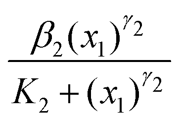 , where β2 is the rate constant. Also, K1 and K2 are dissociation constants, γ1 and γ2 represent the Hill coefficients, and ν is the feedback strength. The above reactions lead to the following kinetic equations.
 | (2) |
 | ||
| Fig. 1 (A) A schematic diagram illustrating key phases (G1, S, G2, and M) and their respective checkpoints, which regulate the progression of the cell cycle. The G1 checkpoint ensures the conditions are favorable for DNA replication before entering into the S phase, where DNA replication occurs. The G2 checkpoint ensures the completion of DNA replication and checks for DNA damage before the cell enters the mitotic (M) phase. The Cdc2-cyclin B complex and Wee1 kinase are responsible for the regulation of the G2 checkpoint, and inhibit each other. When the population of active Cdc2-cyclin B is high, the cell will progress from the G2 phase to the M phase. (B) The inline depiction highlights that the direction of CSD may vary in the vicinity of the tipping threshold. Notably, the CSD direction may also differ for the forward and backward direction, underscoring the complex regulatory mechanisms governing the dynamics of the cell cycle. | ||
Both xi's and yi's are the fractions of the species that form the two conserved relations, x1 + x2 = 1 and y1 + y2 = 1, i.e., the total concentration of both Cdc2 and Wee1 is fixed in the entire system. The fraction of the active concentrations of the Cdc2-cyclin B and Wee1 can be written as:
 | (3) |
The bifurcation analysis of the model (3) with variation in the feedback strength ν (other parameter values are given in Table S1, ESI†) shows that in a certain parameter range, the system exhibits three equilibrium points: two stable equilibrium points and a saddle point intermediate between the two stable points, as illustrated in Fig. 2. The saddle point forms the basin boundary between the two alternative stable equilibrium points. Systems with alternative stable points may exhibit a regime shift. While a parameter gradually moves toward a tipping point, known as a bifurcation point, where such systems suddenly become unstable and shift to another alternative stable state. Specifically, the bifurcation diagram in Fig. 2 reveals the change in steady-state population of Cdc2-cyclin B and Wee1 for different values of ν. It shows that bistability and fold bifurcation exist in the system, and thus, the system can tip from one steady state to another. For low values of ν, i.e., a high Cdc2-cyclin B and a low Wee1 active state, represent the G2 phase of the cell cycle, and the high values of ν, i.e., a low Cdc2-cyclin B and a high Wee1 active state, represent the M phase of the cell cycle. Close to the tipping point, a tiny change in ν or fluctuations in the steady-state population due to noise may trigger a sudden transition.
 | ||
| Fig. 2 Bifurcation diagram for the deterministic Cdc2-cyclin B/Wee1 model. Feedback strength (ν) is the bifurcation parameter. Panel (a) shows the bifurcation diagram for x, and panel (b) shows the bifurcation diagram for y. Solid blue lines represent stable states (high x and low y represent the G2 phase-like state and low x and high y represent the M phase-like state), while the dotted red lines represent the unstable state. The parameter values are: α1 = α2 = 1, β1 = 200, β2 = 10, K1 = 30, K2 = 1, and γ1 = γ2 = 4. The feedback strength ν is varied from 0.2 to 2.0. The tipping points, where the critical transition occurs, are marked by circular beads. | ||
2.2 Theoretical background for the CSD and NSD directions
The chosen model (3) exhibits bistability, which results in the possibility of forward and backward sudden transitions between the G2 phase and the M phase with increase and decrease in ν, respectively. As already discussed, CSD plays a key role in predicting these transitions and has a directional property. Therefore, one has to first determine the leading variable, which is to be monitored among all the variables to get the best signal of an impending transition, employing the directional property of CSD.To identify the direction of the CSD in the Cdc2-cyclin B/Wee1 biochemical system, we first determine the Jacobian matrix (J) near an equilibrium point (x*,y*). For model (3), J is a 2× 2 matrix, and its elements can vary as a function of ν. Out of two eigenvalues of J, let λd be the least negative eigenvalue (dominant eigenvalue) that contributes most to CSD. Corresponding to λd, the right and left eigenvectors, vr and vl, respectively, can be determined. The right eigenvector, vr of λd, is defined as the CSD vector, as this vector gives the direction along which the return rate is approaching zero. The return rate is the speed (rate) at which the system returns back to its equilibrium state after being perturbed. In the proximity of the tipping point, this return rate decreases (becomes zero at the tipping point), and the steady state variance in the direction of critical slowing down grows. The left eigenvector vl of λd is defined as the noise-sensitive vector, as it determines the noise-sensitive direction. To understand the alignment of CSD and NSD, we compute their angles with the state variables axes (1,0) and (0,1), corresponding to species x and y, respectively. The biochemical species vector, which makes the least angle with the CSD vector, is considered the observation direction (OD) and is monitored for EWS. For example, the angle θx between the CSD vector (vr) and the state vectors x and the angle θy between vr and the state vectors y are calculated as:
 | (4) |
 . A value of θ (for x and y) close to zero indicates stronger alignment with the CSD vector, and thus, the monitored protein ought to provide stronger EWS of an impending transition. Furthermore, near the tipping point, the angle between the observation direction and the CSD vector increases if it is not robust enough to forewarn a sudden transition. We present details of the calculation of the angle between the CSD vector and Cdc2-cyclin B and Wee1 in the ESI† (Section S1).
CSD direction is one of the four important directions from which one can identify a sensitive protein for best EWS. However, their simultaneous analyses provide a road map for robust prediction of the most sensitive protein toward EWS. Apart from the CSD direction, the other three are: (a) the primary noise direction (PND) along which the noise is introduced externally, (b) the noise sensitive direction (NSD), which is the vl, and (c) the observation direction (OD), along which the detection is performed.22
The EWS becomes weak if the PND and NSD are nearly orthogonal. In other words, the most informative protein whose direction is parallel to the CSD, but if PND and NSD are nearly orthogonal, it may incorrectly predict critical transitions. Thus, one can propose that the best possible protein for predicting critical transitions through EWS analyses would be the parallel arrangement of (a) the OD and CSD vectors and (b) the PND and the NSD vectors. Similar to the angle between the direction of CSD and observation directions, the angle between the NSD and PND can be calculated by utilizing the left eigenvector vl corresponding to the dominant eigenvalue λd (details are provided in Section S1, ESI†).
2.3. Sensitivity analysis
We calculate the angle between the CSD direction and the biochemical species x and y across a range of parameters. Specifically, with variations in one of the rate constants α1, α2, β1, and β2, along with the bifurcation parameter (ν). In the range of parameter values where the system exhibits bistability, two distinct steady states exist, denoted as and
and  . Here,
  corresponds to a state with active Cdc2 and inactive Wee1, whereas
  corresponds to a state with inactive Cdc2 and active Wee1. The angle between the CSD vector and these two steady states can be expressed as follows:
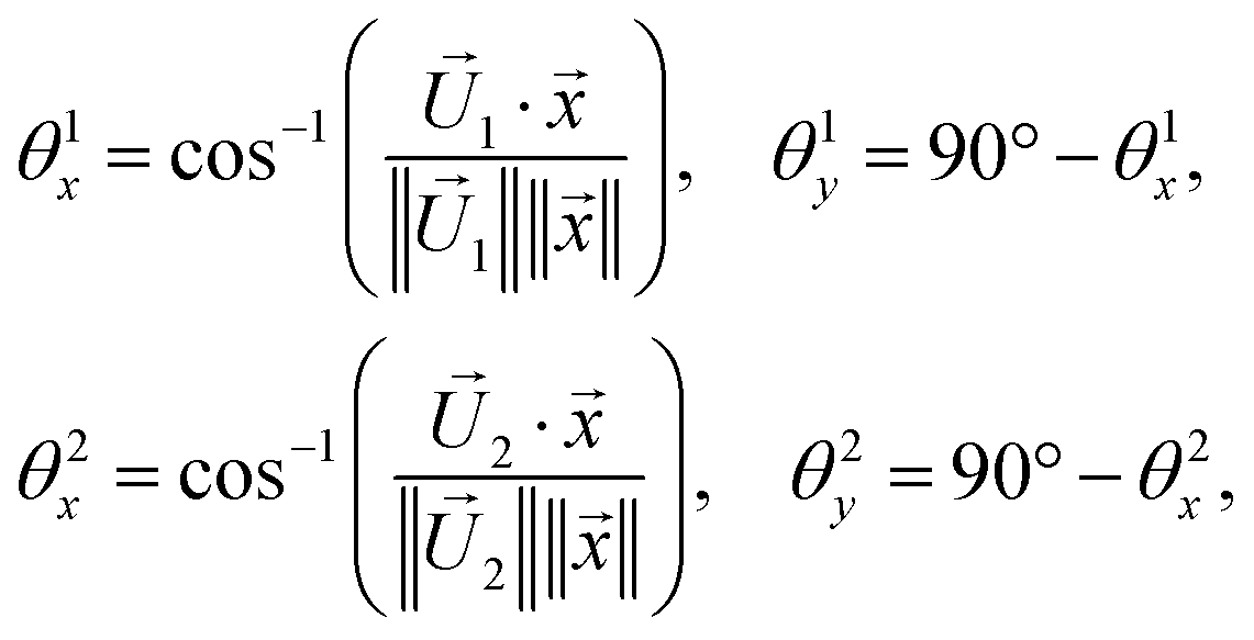 | (5) |
 is the norm of the vector
 ![[x with combining right harpoon above (vector)]](https://www.rsc.org/images/entities/i_char_0078_20d1.gif) , and
, and ![[U with combining right harpoon above (vector)]](https://www.rsc.org/images/entities/i_char_0055_20d1.gif) 1 and 2 represent the right eigenvectors of the dominant eigenvalue of the Jacobian corresponding to the steady states
1 and 2 represent the right eigenvectors of the dominant eigenvalue of the Jacobian corresponding to the steady states  and
and  , respectively.
2.4 Governing stochastic differential equations (SDEs)
Investigating a nonlinear system in the presence of noise is crucial since noise is inevitable in any natural system. We incorporate multiplicative noise into the model, ensuring that noise intensity scales up with the magnitude of the species. This formulation ensures that the stochastic fluctuations in x are more pronounced when x is large, while fluctuations in y increase with the magnitude of y.The model (3) in the presence of multiplicative noise can be written incorporating a stochastic term in the following form:
 | (6) |
2.5 Principal component analysis
As the complexity of a system increases, identification of the OD to forewarn a critical transition becomes challenging. In such cases, principal component analysis (PCA) is an objective and data-driven approach.However, it is crucial to frame the significance of the interpretation and applicability of the PCA and the process of identifying the OD. In order to perform the PCA analysis, consider a dataset represented by p-dimensional vectors, (X), and summarize them by projecting them into a lower q-dimensional subspace Y with minimal loss of information. Mathematically, this projection is achieved by constructing the p × p covariance matrix, defined as:
| Cov(Xi, Xj) = 〈(Xi − 〈Xi〉)(Xj − 〈Xj〉)〉 |
Diagonalizing this covariance matrix yields p eigenvalues (λ) and corresponding p orthogonal eigen directions Y. These p eigenvectors serve as a new basis onto which the original data can be projected to maximize the variance, which can be reordered based on the magnitude of the eigenvalues. The data set projected on the first principal eigen direction corresponding to the largest eigenvalue gives us the first principal component. Therefore, the calculation allows us to identify the most informative directions, with the first principal component corresponding to the direction of maximum variance. For our case, to perform PCA, the two stochastic trajectories were combined into a matrix X such that:
 | (7) |
The corresponding covariance matrix A is constructed. Here, the covariance matrix can be written as:
 | (8) |
 | (9) |
![[x with combining macron]](https://www.rsc.org/images/entities/i_char_0078_0304.gif) and ȳ represent the mean values along the columns of X, and n is the sample size.
and ȳ represent the mean values along the columns of X, and n is the sample size.
The first principal component (PC1) is then determined as the eigenvector associated with the largest eigenvalue corresponding to A, indicating the direction in space where the data points exhibit the most significant variance. Then, the variance along the PC1 direction is calculated. The PCA-based directional analysis is inherently statistical, which allows one to apply it to multivariate complex time series data. We also aim to explore the correlation between PCA and CSD-based methods for our system, if any exists.
3 Results
3.1 EWSs for transitions at G2 phase
Fig. 3(a) and (c) illustrate the temporal progression of the cell cycle, capturing the dynamic transition between active Cdc2-cyclin B and active Wee1 populations, or G2 phase to M phase and vice versa, driven by gradual variations in the feedback strength ν. | ||
| Fig. 3 Stochastic time series embedded on the bifurcation diagram for the forward (a) and backward (c) directions as the value of feedback strength (ν) is progressively increased and decreased, depicted by the black arrow, respectively. Early warning signals (EWS) are highlighted by a significant increase in variance (b) and (d) prior to the tipping point. The rise in variance serves as a predictive indicator of the impending critical transition in the system. The strengths of the noise in x and y are σ1 = σ2 = 0.5. | ||
We generate a large number of stochastic trajectories of (3) for values of ν between 0.2–2.0 and calculate the variance for each stochastic trajectory. The evaluation of the variance of the Cdc2-cyclin B and Wee1 populations within their stochastic time series, prior to the onset of the transition, unveils a marked increase, as presented in Fig. 3(b) and (d). This escalation serves as a compelling indicator of an imminent, abrupt shift. However, the increase in variability for the Cdc2-cyclin B population is much more significant than the slight increase in Wee1 population variability. Importantly, the identification of CSD-based EWS is regulated by the Cdc2-cyclin B but not necessarily by the Wee1 population. We now aim to substantiate our understanding of the underlying mechanisms, highlighting the vital role of Cdc2-cyclin B in driving and predicting this cellular transition. Furthermore, a decrement of the parameter ν gives rise to another critical transition (i.e., G2 delay or arrest), and the variance increases for Cdc2-cyclin B and Wee1. This means that Cdc2-cyclin B and Wee1 regulate the CSD-based indicator for this critical transition. Therefore, a question remains to be identified: What is the critical protein among Cdc2-cyclin B and Wee1 to be monitored (or used for the critical transition analysis) for a robust prediction of tipping in this biochemical switch?
3.2 Observation direction: Cdc2-cyclin B or Wee1?
The sudden decrease in Cdc2-cyclin B complex population can significantly impair the execution of mitosis,33 which may imply errors such as chromosome missegregation. As a consequence, it becomes imperative to proactively anticipate fluctuations in protein populations before they manifest. Accordingly, our investigation is directed toward elucidating the underlying mechanisms that can serve as early indicators of compromised cell functionality within the cell cycle. We, therefore, examine the critical slowing down vectors near the tipping point to determine the observation direction, which serves as a proxy of an upcoming sudden transition in complex systems.The arrows in Fig. 4 depict the direction of the CSD vector in Cdc2-cyclin B/Wee1 interaction for various values of feedback strength ν. The panels on the left are evaluated for changing the ν from low to high values, while the panels on the right are investigated by changing the ν values in the backward direction (high to low). We determine θx when monitoring the Cdc2-cyclin B population and θy when observing the Wee1 population by measuring the angle between the CSD vector and the observation direction. The CSD vectors near and away from the tipping point are presented in Table S2 (ESI†). A more comprehensive plot illustrating the variations in CSD vectors with respect to ν is presented in the ESI† (Fig. S1).
 | ||
| Fig. 4 Comparative analysis of CSD Vectors near and away from the tipping points. The plot illustrates the change in CSD vectors with variations in the feedback strength ν. Notably, in the forward direction (as ν is increased), the CSD vectors align with x in the vicinity of the tipping point, suggesting a predominant influence along this direction. Conversely, in the backward direction (as ν is decreased), the CSD vectors exhibit almost equal alignment with both x and y near the tipping point, highlighting a distinct directional preference. | ||
When ν is low, and the system is in an activated Cdc2 state, the CSD vector aligns with the observation of Cdc2-cyclin B but diverges from the Wee1 observation direction. As we increase ν and approach the tipping point, the angle between the CSD vector and the observation direction shifts. Near the transition, θx increases while θy decreases. However, the CSD direction remains primarily aligned with the observation direction, Cdc2-cyclin B, rather than Wee1. This underlines the mechanism of identifying the early warning signal when monitoring the Cdc2-cyclin B population but not Wee1.
We further investigate the CSD vector in the reverse direction, tracking changes in ν values until we reach the threshold at which the cell recovers from G2 arrest and transitions into the G2 to M progression. For a high ν ≈ 1.7 value, considerably distant from the tipping threshold, the CSD vector aligns significantly with the observation of Wee1 levels. As ν gradually changes to lower values, we observe a shift in the direction of the CSD vector. In this scenario, approaching the tipping threshold (ν ≈ 0.2), the CSD vector aligns nearly equally with the state variable axes corresponding to Cdc2-cyclin B and Wee1. Therefore, changes in the variance of both Cdc2-cyclin B and Wee1 populations can serve as an indicator of an upcoming recovery from G2 arrest in the cell cycle. Importantly, our analysis of the interplay between CSD vectors and OD underscores the importance of prioritizing different variables based on the specific transition pathway under consideration.
3.3. Impact of noise direction on transitions among G2 and M phase
Stochasticity plays a key role in affecting the dynamics of biological and biochemical processes,34,35 which can further influence the detection of early warning signals. It is quite natural that both proteins will not experience the same level of stochasticity; instead, the stochasticity acts heterogeneously. To explore the effect of this heterogeneous stochasticity, we introduce multiplicative noise along Cdc2/cyclin B and Wee1 PND. As mentioned before, if the PND and NSD are orthogonal to each other for a protein, then it may not be a suitable monitoring protein for the identification of a tipping event. We evaluate how stochasticity impacts the EWSs along the CSD vectors in the Cdc2-cyclin B/Wee1 biochemical switch. In Fig. 5(a), we show that in the forward direction, as ν is increased, stochasticity in the Wee1 population has no impact on the variance of either of the state variables. In the realm of cellular function, it is of significance to recognize that monitoring the levels of either Cdc2-cyclin B or Wee1 does not offer a reliable means of promptly detecting the transition.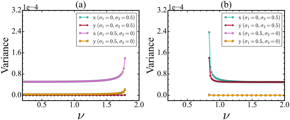 | ||
| Fig. 5 Effect of noise strength on EWS performance in the forward (a) and backward (b) directions as the value of ν is increased and decreased, respectively. The strength of EWS is observed to increase with the increment of noise strength (σ1 for the forward direction and σ2 for the backward direction). This figure illustrates the contrasting impact of the direction of noise on the EWS in both directions. | ||
In contrast to this outcome, external stochasticity in the Cdc2-cyclin B level gives rise to an increase in variance. Also, it depicts that treating Cdc2-cyclin B but not Wee1 as an observation variable is a reliable indicator of an upcoming critical transition, indicating that the observation direction remains the same.
However, a gradual change of ν from 2.0 to 0.2 increases the variances in both Cdc2-cyclin B as well as Wee1 proteins, when noise is added along the Wee1 protein, as shown in Fig. 5(b). The above findings can be explained by the direction, which is called the noise-sensitive direction (NSD). For the forward direction, the NSD is aligned more with the Cdc2-cyclin B direction in the cell, while the NSD is aligned with Wee1 for the backward direction. The NSD vectors near and away from the tipping point are presented in Table S3 (ESI†). Also, a comprehensive plot illustrating the variations in NSD vectors with change in ν is also presented in Fig. S2 (ESI†).
3.4 Sensitivity analysis
Complexity, where numerous parameters govern system dynamics, is an inherent characteristic of biological systems. It is, therefore, imperative to focus on the robustness of our outcomes towards changes in the various parametric conditions in the Cdc2-cyclin B/Wee1 cell functioning. Fig. 6 and 7 show the change in θx as the system reaches the bifurcation point for a range of values of the kinetic parameters (α1, α2, β1, and β2) along with the variation of bifurcation parameter values, ν. | ||
| Fig. 6 The angle the CSD vector makes with x (θx) is plotted with variations in parameters α1, α2, β1 & β2 and the strength of the feedback ν for the forward direction. Panels (a)–(d) correspond to variations in α1, α2, β1 & β2, respectively. The two black lines represent the set of saddle-node points, and the black arrow represents the direction of change of ν. θ < 45° before the transition suggests that x is the dominant sensitive protein and will give a more pronounced increase in variance before the tipping point. | ||
 | ||
| Fig. 7 The angle the CSD vector makes with x (θx) is plotted with variations in parameters α1, α2, β1, & β2 and the strength of the feedback ν for the backward direction (as ν is decreased). Panels (a)–(d) correspond to variations in α1, α2, β1 & β2, respectively. The two black lines represent the set of saddle-node points, and the black arrow represents the direction of change of ν. θx > 45° before the transition suggests that y is the dominant sensitive protein as θy = 90°−θx and will give a more pronounced increase in variance before the tipping point. | ||
The black lines denote a series of saddle-node bifurcation points, and the region between these curves indicates the bistability region, beyond which the system exhibits a transition from one state to another, indicating critical transitions as the parameters vary. A detailed three-dimensional illustration of the saddle-node bifurcation with observation variable x and the ν and β2 is shown in Fig. S3 (ESI†).
As the value of ν increases, the solid line on the right-hand side indicates G2 arrest. Variation in the kinetic parameters alters the bifurcation threshold value of ν, as indicated by the solid line.
Fig. 6 illustrates that before the critical transition, the CSD direction for the variation in all the kinetic parameters α1, α2, β1, & β2 remains aligned more with Cdc2-cyclin B and does not change much (pink color region). However, we find a sharp change in θx and it becomes orthogonal upon further increase of ν (green color region). Note that the effect of the variation of all the kinetic parameter values on the θx is similar, implying that they affect the critical transition homogeneously. Therefore, selecting Cdc2-cyclin B is more appropriate for detecting the critical transition as the value of ν is increased and the system remains insensitive to the kinetic parameters. This implies that besides knowing the most suitable observation variables, understanding parametric sensitivity is critical for detecting critical transition.
Also, as the value of ν decreases, as happens in the backward transition, the solid line on the left demonstrates the recovery of the cell functioning from G2 arrest.
Fig. 7 illustrates that before the critical transition, the CSD direction remains aligned more with Wee1 for the variation of all kinetic parameters until it hits the bifurcation point (solid black line). However, near the bifurcation point, the CSD vector changes its orientation and is aligned almost equally with the Cdc2-cyclin B and Wee1. Unlike the forward transition, the angle change is not sharp for the backward direction, as evidenced by the faded green color near the transition point. The results imply that the chosen observation direction is not unique to the transition point for the backward direction. Our analysis shows that the effect is almost similar for the variation of all the kinetic parameters. Furthermore, the kinetic parameters alter the bifurcation threshold but do not affect the angle between the CSD and the OD. Thus, understanding the EWS in both Cdc2 and Wee1 levels is robust to system parameters for varying values of the bifurcation parameters.
3.5 Principal component analysis
We showed that aligning the OD and CSD vectors provides a clue for identifying the most sensitive species that govern the significant disturbances before the transition. However, calculating CSD for a dynamical system is limited since the quantity is nothing but the dominant eigenvector of the Jacobian of the linearized system. Thus, prior knowledge of the model equation is required to calculate the Jacobian and the CSD. However, in many practical instances, the system's dynamics may be described by time series data of a vector constituted by a set of dynamical variables without knowing the model equations. Therefore, we look for an alternative method that bypasses the calculation of CSD. As demonstrated before, detecting a tipping point identifies maximum variance along the direction in which critical transition occurs. In this spirit, the principal component analysis (PCA) may serve this purpose as the method maximizes the variances along the first principal direction (PC1). The PCA method is a statistical technique used to reduce the dimensionality of a data set while retaining as much information as possible.36 We conducted PCA on a time series generated from the stochastic simulation23 and calculated the variance in the direction of the first principal component (PC1) for the stochastic trajectories. In order to carry out this calculation, we first calculate the PC1 from the stochastic trajectory and then project it on the PC1. We calculate the variance from the projected trajectory for the forward and backward transitions, and the results are presented in Fig. 8. We observe an increase in variances near the tipping point, indicating an upcoming critical transition for our data set. In other words, PC1 serves the same role as the CSD vector for time series data. Therefore, we can use PC1 as a reference direction for detecting the critical transition for time series data.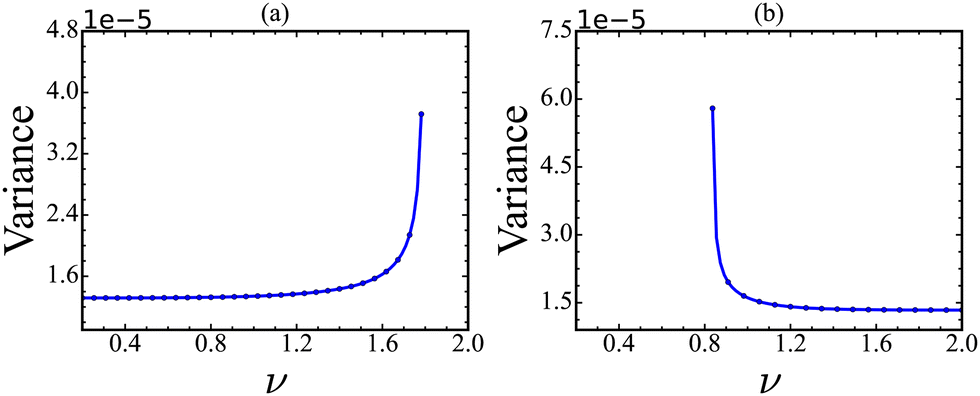 | ||
| Fig. 8 The projected trajectories are used to calculate the variance along the forward and backward directions by varying the value of feedback strength (ν). Early warning signals (EWS) are highlighted by a significant increase in variance (a) and (b) prior to the tipping point. The rise in variance is a predictive indicator of the impending critical transition in the system. | ||
In the following step, we find the species most related to the first principal component. Note that PC1 is a linear combination of unit vectors associated with the dynamical variables. The square of each component (vi2) is the probabilistic contribution of that variable to the PC1, and it plays a crucial role in identifying the most sensitive species for a critical transition. In other words, the species most related to the first principal component could be the OD with the strongest expected trends in variance prior to transition. We plot the square of the components (v12 and v22) of PC1 as a function of ν and present them in Fig. 9. It is clear from the analyses that the Cdc2-cyclin B contributes more to the PC1 than the Wee1 for the transition along the forward direction near the tipping point. However, both proteins contribute equally to the PC1 for the backward direction near the tipping point. These results correlate well with the results obtained from the CSD-based analysis, where we find that the Cdc2-cyclin B is the most suitable OD for detecting the critical transition in the forward direction. However, we do not have such a choice in the backward direction since both proteins contribute almost equally to the PC1. The results are further supported by the angle alignment between PC1 and ODs, as shown in Fig. 10. In the forward direction, the Cdc2-cyclin B is aligned more (the angle ranging between 13.4 to 22.4°) with the PC1 up to the tipping point and exhibits an abrupt jump in angle at the tipping point. However, we find both Cdc2-cyclin B and Wee1 aligned to the PC1 at an angle of ≈ 45.0° in the backward direction, indicating the difficulty of choosing the species for detecting the transition. Nevertheless, we find that both results obtained from CSD and PC1 correspond with each other, suggesting that one can perform PCA-based analyses for time series data to identify the most sensitive species toward the detection of a critical transition.
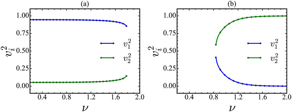 | ||
| Fig. 9 The plot of the probabilistic contribution of the species as given by the square of the components of PC1 (v1 and v2) for x (panel (a)) and y (panel (b)) species, as a function of the feedback strength, ν. The contribution of the species x to the PC1 near the tipping point is much larger than the species y for the forward direction, which indicates that x could be the monitoring species. In the backward direction, both species contribute equally to the PC1 near the tipping point, demonstrating the difficulty of choosing a monitoring species for predicting the critical transition. | ||
 | ||
| Fig. 10 The alignment of OD with PC1 vectors near and away from the tipping points is shown. Similar to CSD vectors, as the value of ν is increased, the PC1 vectors align with x in the vicinity of the tipping point. Also, as the value of ν is decreased, the PC1 vectors align almost equally with x and y. | ||
4 Generality of the proposed method
In the previous sections, we demonstrated how to choose a specific protein to accurately forecast a sudden transition for the G2/M transition in a cell cycle. The results obtained from our proposed methods are promising. We have identified CdC2-cyclin B protein as the best monitoring species for foreseeing such transitions. However, one may argue that the chosen system is low-dimensional, so the proposed doctrine may not work efficiently for a higher-dimensional system. In order to eliminate such an argument and its applicability to a wide range of systems, we chose a three-dimensional system where we have also identified the monitoring species for a critical transition.We chose a well-known regulatory network model in cancer biology that governs the epithelial (E) to mesenchymal (M) transition and vice versa (EMT and MET). The transition becomes vital in cancer progression since the solid tumors originate in epithelial organs (localized E state) that undergo a phase transition where they lose cell–cell adhesion (mobile M state) and gain the traits of migration and invasion. Cells undergoing EMT get launched into the bloodstream and also gain the ability to initiate new tumors at metastatic sites and gain resistance against multiple drugs. The core regulatory network of this system is a three-dimensional microRNA (miR) based chimeric circuit developed by Lu et al.,24 and we present the model in the ESI† (eqn (S19)–(S21)). The model received considerable attention since it exhibits tristability and captures a hybrid E/M phenotype, which may be more aggressive for cancer progression.3
The system exhibits tristability as shown in the bifurcation diagram Fig. S6 (ESI†), where the protein ZEB is chosen as the state variable and the protein SNAIL as the driver parameter. The stochastic trajectory is embedded in the bifurcation diagram and shows the existence of two abrupt transitions, namely E → E/M and E/M → M in the forward direction. However, the system exhibits an abrupt transition in the backward transition but bypasses the E/M phenotype state. In Fig. S7 (ESI†), we analyze the variances of the three species (miR200(μ200), mRNA (mZ) and the protein ZEB (Z)) as a function of SNAIL for the two transitions along the forward direction (panels a and b) and the transition along the backward direction (panel c). The results demonstrate that Z shows the highest level of variance around the tipping point compared to the other two biochemical species. This result also suggests that the CSD direction must align more with the Z OD. In this regard, we calculate the angle (θs) between the CSD and ODs associated with all three species. We present the result in Table S4 (ESI†). We find that Z is aligned more with the CSD near the tipping point of the E-state (19.5°), and it continues to align up to the tipping point of the hybrid E/M state (2°), and it remains aligned with the backward CSD vector for the M → E tipping point (0.3°). The alignment of CSD and the OD along the Z protein excludes other monitoring species for identifying the critical transition.
We perform a similar PCA-based stochastic trajectory analysis as we did for the G2/M transition to identify monitoring species for the EMT. We calculate the PC1 vector from the stochastic trajectory of this system. Similarly, as we have done for the G2/M transition, we project the original stochastic trajectory on the PC1 and calculate the variance from there (Fig. S7, ESI†). We find the variance near the tipping point of all the transitions, a clear sign of the critical transition in the data. We calculate the square of each component of the PC1 for all three transitions, and the results are shown in Fig. S9 (ESI†). The results demonstrate that the Z contributes more to constructing the PC1 near the tipping point for all three transitions. The results are further validated by calculating the angles (ϕs) between Z and PC1 for all three transitions, and the results are presented in Table S4 (ESI†). Similar to the results obtained for the CSD vector, the PC1 also identifies that the Z aligns more (ϕZ = 40.0°, 0.6° and 2.3°) with the PC1 near the tipping point for all three transitions. Therefore, the PC1 and CSD vectors also complement each other for this higher dimensional system, and maybe the PC1 based on analysis works uniquely in identifying the critical transition and the monitoring species from time series data.
5 Conclusions
In this paper, we demonstrate the importance of CSD, NSD, PND, and OD vectors in detecting critical transitions in the Cdc2-cyclin B/Wee1 cell cycle model system. We analyze these directions systematically and find that the alignment of OD with CSD, as well as with NSD and PND, provided a roadmap for the robust detection of critical transitions. First, we propose a method for identifying key monitoring species that can reliably predict critical transitions in complex biochemical systems. We identified the direction of CSD and measured EWSs along this direction. Our results demonstrate that measuring EWSs in alignment with the CSD direction provides a more dependable indication of an impending critical transition. Furthermore, incorporating noise along the NSD or with species that align more with the NSD enhances the intensity of the EWS indicator. Second, our calculations complement the PCA-based method, which relies solely on stochastic trajectories. We find that the first principal direction correlates well with the CSD direction. Therefore, measuring EWS along the first principal direction of a time series serves the same purpose as measuring that along the CSD direction. It is important to note that the PCA-based method does not require any model equations, as it analyzes data derived from time series (stochastic trajectories). Since the CSD and PCA-based methods complement one another, it is possible to predict critical transitions in any time series data. Such analyses can be valuable for detecting sudden transitions in multidimensional time series datasets. Third, we validated our proposed method using a three-dimensional dynamical system and predicted that monitoring the ZEB protein would yield the most effective predictions for the epithelial–mesenchymal transition.Specifically, our analysis shows that the monitoring protein may differ in the direction of critical transitions. This happens because the direction of the CSD vector near the tipping point depends on such directions. We have shown that variances (EWS) for the Cdc2-cyclin B and Wee1 increase near the tipping point for the G2 to M transition and vice versa. However, Cdc2-cyclin B is the best monitoring species for the forward transition. However, both proteins are equally preferable for the backward transition after rigorous analysis of the direction of various vectors. Our analyses show that CdC2-cyclin B is aligned more with the CSD vector near a tipping region, which increases the variance values significantly. However, we have not found any such preference in protein selection for the backward transition from our analysis, as both proteins align almost equally with the CSD vector. Additionally, systems with multiple parameters may give false positive critical transitions upon their variation. In this regard, our sensitivity analysis shows that the increase in variances for the identified species near a tipping point is almost unaffected by the kinetic parameter variation, demonstrating our calculation's robustness. Furthermore, we find that the first principal direction (PC1) from the PCA analysis complements the CSD-based calculations. We show that the species contributing more to constructing PC1 is the best monitoring species. Since the PCA analysis is done only on the stochastic trajectory, we find Cdc2-cyclin B as the best monitoring species for the forward transition. However, we are silent in choosing the best species in the backward direction since Cdc2-cyclin B and Wee 1 align equally with the PC1 vector. The PCA-based method may also identify a critical transition directly from multidimensional time series data. However, one must perform similar calculations for various systems to establish such complementarity between CSD and PC1-based methods.
Lastly, we put effort into establishing our proposed method for general applicability to a wide range of problems. In this regard, we chose the EMT system that exhibits critical transition. This dynamical system differs from the G2/M transition as it has three variables and exhibits tristability. We apply our method to this system and perform all possible directional analyses to identify the monitoring species for forward and backward transitions as a function of SNAIL concentration. We identify a unique protein, ZEB, which may be the best monitoring species to identify a critical transition from a time series data set or from an experiment. Like the G2/M transition, we perform PC1-based directional analysis and again establish the complementarity between PC1 and CSD vectors. Overall, our analyses may be used as an algorithm to identify monitoring species for the robust and efficient prediction of critical transitions in a natural system. However, to determine the CSD direction in a dynamical system that exhibits long transient oscillations before shifting to an alternative state can be a challenging and interesting future research question.25
Data availability
Data and relevant codes for these analyses are available at: https://doi.org/10.5281/zenodo.14269612 and in the ESI.†Conflicts of interest
There are no conflicts of interest to declare.Acknowledgements
D. K. acknowledges the financial support from IIT Ropar. S. K. S. is supported by SERB, Department of Science and Technology, Government of India (MTR/2020/000553) and (CRG/2022/000345).References
- C. Trefois, P. M. Antony, J. Goncalves, A. Skupin and R. Balling, Curr. Opin. Biotechnol., 2015, 34, 48–55 CrossRef PubMed.
- R. Liu, M. Li, Z.-P. Liu, J. Wu, L. Chen and K. Aihara, Sci. Rep., 2012, 2, 813 CrossRef PubMed.
- S. Sarkar, S. K. Sinha, H. Levine, M. K. Jolly and P. S. Dutta, Proc. Natl. Acad. Sci. U. S. A., 2019, 116, 26343–26352 CrossRef PubMed.
- M. Scheffer, S. Carpenter, J. A. Foley, C. Folke and B. Walker, Nature, 2001, 413, 591–596 CrossRef PubMed.
- E. Á. Hernández, S. Kahl, A. Seelig, P. Begovatz, M. Irmler, Y. Kupriyanova, B. Nowotny, P. Nowotny, C. Herder and C. Barosa, et al. , J. Clin. Invest., 2017, 127, 695–708 CrossRef PubMed.
- J. D. Touboul, A. C. Staver and S. A. Levin, Proc. Natl. Acad. Sci. U. S. A., 2018, 115, E1336–E1345 CrossRef.
- A. Kianercy, R. Veltri and K. J. Pienta, Interface Focus, 2014, 4, 20140014 CrossRef.
- I. A. van de Leemput, M. Wichers, A. O. Cramer, D. Borsboom, F. Tuerlinckx, P. Kuppens, E. H. Van Nes, W. Viechtbauer, E. J. Giltay and S. H. Aggen, et al. , Proc. Natl. Acad. Sci. U. S. A., 2014, 111, 87–92 CrossRef.
- L. Lahti, J. Salojärvi, A. Salonen, M. Scheffer and W. M. De Vos, Nat. Commun., 2014, 5, 4344 CrossRef.
- M. Scheffer, J. Bascompte, W. A. Brock, V. Brovkin, S. R. Carpenter, V. Dakos, H. Held, E. H. Van Nes, M. Rietkerk and G. Sugihara, Nature, 2009, 461, 53–59 CrossRef PubMed.
- M. C. Boerlijst, T. Oudman and A. M. de Roos, PLoS One, 2013, 8, e62033 CrossRef PubMed.
- J. A. Perry and S. Kornbluth, Cell Div., 2007, 2, 1–12 CrossRef.
- A. Fattaey and R. N. Booher, Prog. Cell Cycle Res., 1997, 233–240 CrossRef.
- A. I. Laskin, J. W. Bennett and G. M. Gadd, Advances in applied microbiology, Academic Press, 2003 Search PubMed.
- I. Kovalchuk and O. Kovalchuk, Genome stability: from virus to human application, Academic Press, 2021, vol. 26 Search PubMed.
- E. Senturk and J. J. Manfredi, p53 Protocols, 2013, pp. 49–61 Search PubMed.
- W. J. Lennarz and M. D. Lane, Encyclopedia of biological chemistry, Academic Press, 2013 Search PubMed.
- J. H. Chung and F. Bunz, PLoS Genet., 2010, 6, e1000863 CrossRef PubMed.
- C. J. Matheson, D. S. Backos and P. Reigan, Trends Pharmacol. Sci., 2016, 37, 872–881 CrossRef.
- Y.-Y. Lee, Y.-J. Cho, S.-W. Shin, C. Choi, J.-Y. Ryu, H.-K. Jeon, J.-J. Choi, J. R. Hwang, C. H. Choi and T.-J. Kim, et al. , Sci. Rep., 2019, 9, 15394 CrossRef PubMed.
- F. Esposito, R. Giuffrida, G. Raciti, C. Puglisi and S. Forte, Int. J. Mol. Sci., 2021, 22, 10689 CrossRef PubMed.
- A. C. Patterson, A. G. Strang and K. C. Abbott, Am. Nat., 2021, 198, E12–E26 CrossRef.
- V. Dakos, Ecol. Indic., 2018, 94, 494–502 CrossRef.
- M. Lu, M. K. Jolly, R. Gomoto, B. Huang, J. Onuchic and E. Ben-Jacob, J. Phys. Chem. B, 2013, 117, 13164–13174 CrossRef.
- C. J. Ryzowicz, R. Bertram and B. R. Karamched, Phys. Chem. Chem. Phys., 2024, 26, 24861–24869 RSC.
- A. Hastings, K. C. Abbott, K. Cuddington, T. Francis, G. Gellner, Y.-C. Lai, A. Morozov, S. Petrovskii, K. Scranton and M. L. Zeeman, Science, 2018, 361, eaat6412 CrossRef PubMed.
- S. Kéfi, V. Dakos, M. Scheffer, E. H. Van Nes and M. Rietkerk, Oikos, 2013, 122, 641–648 CrossRef.
- D. Angeli, J. E. Ferrell Jr and E. D. Sontag, Proc. Natl. Acad. Sci. U. S. A., 2004, 101, 1822–1827 CrossRef PubMed.
- B. Novak and J. J. Tyson, J. Cell Sci., 1993, 106, 1153–1168 CrossRef PubMed.
- J. R. Pomerening, E. D. Sontag and J. E. Ferrell Jr, Nat. Cell Biol., 2003, 5, 346–351 CrossRef CAS.
- W. Sha, J. Moore, K. Chen, A. D. Lassaletta, C.-S. Yi, J. J. Tyson and J. C. Sible, Proc. Natl. Acad. Sci. U. S. A., 2003, 100, 975–980 CrossRef CAS.
- G. Maruyama, Rend. Circolo Mat. di Palermo, 1955, 4, 48–90 CrossRef.
- K. Riabowol, G. Draetta, L. Brizuela, D. Vandre and D. Beach, Cell, 1989, 57, 393–401 CrossRef CAS PubMed.
- N. G. Van Kampen, Stochastic processes in physics and chemistry, Elsevier, 1992, vol. 1 Search PubMed.
- P. C. Bressloff, Stochastic processes in cell biology, Springer, 2014, vol. 41 Search PubMed.
- M. Greenacre, P. J. Groenen, T. Hastie, A. I. d’Enza, A. Markos and E. Tuzhilina, Nat. Rev. Methods Primers, 2022, 2, 100 CrossRef CAS.
Footnote |
| † Electronic supplementary information (ESI) available. See DOI: https://doi.org/10.1039/d4cp04863f |
| This journal is © the Owner Societies 2025 |