Resistivity mapping of SiC wafers by quantified Raman spectroscopy

Abstract

μRaman spectroscopy measurements were used to study the resistivity in 4H-SiC samples by intercalibrating with Eddy current measurements (eddy-current probe that accurately measures bulk resistivity of wafers). The position and line width associated with the Raman longitudinal optical phonon-plasmon coupled (LOPC) mode were used since their variation from the reference values of a material in the absence of dopant-generated defects is proportional to the amount of the free carrier concentration in the conduction band present in the semiconductor. Using wafers of known resistivity to calibrate the model and deconvolving the individual recorded spectra, a multi-variable model was created to predict the resistivity of individual map points. Resistivity was thus predicted in a pointwise manner resulting in maps of 92 points over a 6-inch diameter area of a wafer, from which false-colour images were created showing the spatial distribution along the X and Y axes, and in the bulk, along the Z axis of the resistivity. The analysis procedure was automated by creating suitable R-language codes that extract the necessary information on the individual aspects of the analysis and create the images described above from a single dataset.

---

1. Introduction

Silicon carbide (SiC) has emerged as an innovative semiconductor material, transforming devices that require high voltage capability and excellent performance even at high temperatures. SiC offers several advantages over traditional silicon-based semiconductors due to its remarkable properties, including its wide band gap, high electrical breakdown range, saturated electron velocity and excellent thermal conductivity.¹ These properties enable SiC-based devices to achieve higher switching frequencies, greater energy conversion efficiency and withstand higher voltages, currents and operating temperatures than conventional devices.² SiC components also have a significantly higher critical breakdown voltage and lower turn-on resistance, which results in higher efficiency through reduced power loss. The advantages of SiC over conventional silicon-based devices, combined with the potential for reduced power consumption and environmental impact, make it a strong choice for a wide range of applications.³ Delving deeper into SiC technology and its implications for semiconductor applications, it is clear that SiC is destined to play an essential role in shaping the future of power electronics. For mapping the surface wafer defects that could impair device operation, several non-destructive approaches have been used such as: (i) teraHertz time-domain spectroscopy (THz-TDS);⁴ (ii) solid-state light sources LED diodes⁵ (UV-C LEDs); (iii) optical techniques;⁶ (iv) optical techniques applied to neural networks;⁷ (v) density-based clustering-based defect pattern analysis method⁸ (DBC) and (vi) four-point microprobes⁹ (M4PP).

μRaman is a powerful method for characterizing silicon carbide crystals because an appropriate choice of excitation laser causes the energy of the electronic band gap of SiC to be greater than the energy of the Ar-ion laser and thus the Raman measurement of a-SiC in the visible region is not disturbed by the presence of luminescence; exceptions are highly doped samples.¹⁰ An example is reported in Tseng et al.^10,11 where an excitation laser in the visible region (532 nm, 2.33 eV) is used rather than lasers in the UV-C region (244 nm, 5.08 eV) chosen in a previous study;¹² in this case, the excitation energy is significantly lower than the band gap of 4H-SiC,¹³ which is 3.24 eV. The low photon energy at 532 nm not only prevents the generation of photoluminescence but also avoids surface damage (alterations) to 4H-SiC by overexposure.

Furthermore, Liu et al.¹⁴ have experimentally verified that no increase in carrier concentration due to photo-generated carriers happens when using a 532 nm laser, or even a 325 nm laser at low power.

In the presence of dopants such as nitrogen, defects are generated with which LO phonon-plasmon coupled (LOPC) are associated, where the LOPC mode is observed when, in a polar semiconductor, a plasmon i.e., the collective excitation of free charge carriers, interacts with the LO phonon via electric fields, generating a Raman-active response.¹² In a LOPC defectivity situation, the LO signal at position 964 cm⁻¹ decreases and broadens asymmetrically.¹⁵ The first-order Raman bands decrease in intensity as the amount of free carriers increases, and broad bands activated by the disorder appear. The position and line width associated with LOPC are modified proportionally to the amount of n-type dopant used in the semiconductor.^14,16 The Raman line shape of the LOPC mode changes significantly with the density of free carriers¹⁷ (n). The present manuscript aims to develop a method for determining the resistivity in different areas of a SiC wafer by Raman analysis, exploiting the ability of free charge carriers to promote current flow, and therefore their effect on the resistivity of the material. The goal is to create a rapid and simple method, which, through analysis without direct contact with the material surface, allows the evaluation of the device's homogeneity or inhomogeneity from an electrical point of view.

2. Experimental

2.1 Materials and methods

We performed this study on samples provided by Global Wafers, they are 6-inch 4H silicon carbide wafers from different bowls, which have resistivity values between 12.5 and 27.3 mΩ cm. The complete list of samples is reported in Table S4 (ESI†).

A typical 4H-SiC Raman spectrum obtained from the literature in the absence of defects, is in the wavenumber range of 100–1200 cm⁻¹ (Fig. 1). It is possible to calculate the symmetry of the vibration modes, through the vector x = q/qB where x is the reduced wave vector of the phonon modes (Table 1);¹² for 4H-SiC in the low-frequency region below 266 cm⁻¹ sharp bands which corresponding to the phonon modes in the transverse acoustic branches (TA) can be observed. Doublet structures are observed for the Folded modes of Transverse Acoustic (FTA); the splitting of the doublets is between 3 to 6 cm⁻¹ and the extent of splitting depends on the experimental setup.¹⁸ The splitting at forward scattering geometry is smaller than for backscattering geometry. This dependence arises from the dispersion of the FTA mode. The Folded modes of the Axial Acoustic branch (FLA) appear as a weak signal and are visible at 610 cm⁻¹. In SiC-4H polytype the Transverse Optic mode (FTO) is split into two signals located at 776 (intense) and 796 (weak) cm⁻¹, while the Axial Optic mode (FLO) shows an intense signal¹² at 964 cm⁻¹ (Fig. 1).

Fig. 1 Typical 4H-SiC Raman spectrum in the frequency range 100–1200 cm⁻¹; adapted from (S. Nakashima¹² et al.).

Table 1 Raman spectra measured with a quasi-back scattering geometry for 4H-SiC; adapted from S. Nakashima¹² et al.

X = q/qB	FTA	FTO	FLA	FLO
0	—	796	—	948
2/4	196, 204	776	—	—
4/4	266	—	610	838

---

Micro-Raman analyses were performed by using a LabRam HR Evolution microscopic confocal Raman spectrometer from Horiba (Horiba Ltd, Kyoto). Micro-Raman spectroscopy was excited by a 532 nm continuous-wave (CW) Nd:YAG laser. The laser beam was focused on a spot whose size was about 0.4 μm² in diameter. The samples were placed on an XYZ stage with 1 μm spatial resolution with an automatic movement system on both x and y-axes as well as z-axes SiC has fairly weak absorption coefficients in the visible region and gives large penetration depth for Raman probe lasers. The literature reported that penetration depth d is roughly evaluated by:

where a is the absorption coefficient. In the context of 4H-SiC at 3.3 eV, and utilising the reported absorption coefficients for high-purity samples, a typical value of d = 2 mm is obtained for visible lasers at a wavelength of 500 nm (2.5 eV photon energy).¹⁹ In addition to this theoretical discussion; to ensure that the penetration depth of the excitation light is limited to the surface region, Tseng¹⁰ et al. suggest gradually decreasing the laser power using this approach; the data reported for an intensity of 1 and 100% indicate a depth of 0.245 and 3.830 μm, respectively, where the power of the light incident at an intensity of 0.12% was the threshold power needed to generate Raman signals. Furthermore, when the depth of light penetration decreases the surface region of the wafer will make a greater contribution to the Raman signal. One way to vary the depth of analysis is also to change the optical magnification; in optical microscopy, the depth resolution (d_f) of a microscope is proportional to:²⁰where λ is the wavelength of laser light and NA is the numerical aperture lens, conventionally indicated on the optical lens (Table S1, ESI†). Using d_f (2) we calculated the different depths of analysis penetration along the Z-axis of the wafer, modifying the magnification, by varying 5 optical lens (100; 80; 50; 20; 10×) shown in Table S1 (ESI†); it is important to remember that this constitutes an approximation since the formula does not include the type of material used. Based on these considerations, we selected a fixed laser power of 10% to obtain spectra with an acceptable signal-to-noise ratio, which allows us adequate numerical treatment on the recorded data sets, for all reported analyses, choosing to always work at the same depth of analysis. Instead, for analyses along the Z axis, we decided to continue to keep the laser power fixed and to vary the NA. The Raman microprobe is very useful for measuring the local area of a sample. Using an NA numerical aperture lens, the diameter of the laser beam focused on the sample surface is given by:

For λ 532 nm and NA 0.75, we obtain D = 0.9 mm. This implies that Raman spectra can be measured with a mm or sub-mm spatial resolution. For Raman microprobe measurement, the experimental geometry is limited to a backscattering geometry; however, the morphology of the sample surface can influence the Raman signal intensity in fact at the same line width considered, a smoother surface will amplify the signals, while rougher surfaces,²¹ such as those of raw wafers or in the early stage of processing, will show weaker signals. In contrast, surface morphology does not affect the relative ratios between signals in the same spectrum; in fact, all bands will be attenuated or intensified, with the same intensity.²¹ For this reason, absolute intensities will not be considered, but the ratio of each individual band to the most intense band in the spectrum. Instead, since the focus of this work is resistivity, the effects of any surface defects were not considered.

The instrumental parameters used are: laser type 532 nm green light, laser power 10%, magnification 80×, bore 100, grating 1800, acquisition time 20 s, accumulation 2 while the area section sampled during a single analysis corresponds to the laser spot diameter (0.7 μm).

For the purposes of data analysis, we utilised the R software environment (an open-source statistical computing and graphics platform, developed under the auspices of the R Project for Statistical Computing).

2.2 Instrument calibration

To perform the μRaman instrument calibration of the 532 nm laser, a certified silicon wafer (Horiba Ltd, Kyoto) with 100× magnification whose spectrum presents an intense band centred at 520 cm⁻¹ is conventionally used. In addition, an internal standard can be used to make the analysis sessions performed in different working sessions comparable, the spectrum of which must present at least one intense signal with a peak in or near the spectral range of interest, but whose signals must not overlap with those of the sample.

For this purpose, the spectral range of analysis was extended for all recorded spectra up to 1850 cm⁻¹ (Fig. 2), and the band at 1702 cm⁻¹ generated by a neon diode was used as the internal standard.

Fig. 2 Raman spectra of selected Neon band at 1702 cm⁻¹, within 4H-SiC spectrum.

2.3 Analysis procedure

The Raman bands of SiC are included in the range between 1200 and 100 cm⁻¹. The spectrum of a sample of SiC-4H wafers (Pol 01) recorded in the range between 100 and 1850 cm⁻¹ is shown in Fig. 2; it can be observed that all typical signals are present, but compared with those reported by Nakashima,¹² a shift of about 8 cm⁻¹ is observed. This behaviour has been observed to be constant for all bands, and it is hypothesised that this could be due to unconsidered factors, such as environmental conditions (e.g. temperature), or instrumental setup. However, these factors are not mentioned in Nakashima's work. Information on resistivity was extracted from all recorded spectra using a curve-fitting procedure and a linear regression model applied to the three components found (see Fig. S2, ESI†). The parameters considered are: the Raman shift which provides information about the position of the band associated with a specific vibrational mode; the relative intensity (i.e., normalized for the most intense peak of the spectrum) of the band used to compare the intensities of the same bands in different spectra and the width of the signal measured at half height or FWHM (full width at half maximum).

The LOPC (longitudinal optical plasmon coupled) Raman band in SiC wafers is correlated with the material's resistivity; this correlation arises because the LOPC mode reflects carrier concentration and mobility, which are directly influenced by doping levels and, consequently, the resistivity. Liu et al.¹⁴ show that as carrier concentration increases, the LOPC band shifts due to plasmon-coupled interactions with lattice vibrations. As an illustration, Raman analysis in SiC has been employed to extend measurements of carrier concentrations down to 5 × 10¹⁵ cm⁻³, thereby facilitating a more comprehensive understanding of the resistivity and uniformity of the material. The curve fitting procedure was performed with the open-source software Fityk for brevity; the complete procedure is reported in ESI.† In order to detect any differences in resistivity, 6-inch silicon carbide wafers, which are commercially available, were employed. The resistivity was then analysed in relation to specific aspects of production, including the variation on the surface of the wafer (X, Y axes) and the variation of resistivity with respect to sampling depth (Z axis). Furthermore, the variation of resistivity at different processing steps was taken into consideration. To evaluate the variation of resistivity on the wafer surface, 92 analysis points distributed uniformly over the surface were chosen and a distance from the edges of 5 mm and a distance between individual points of 10 mm was considered (Fig. 4). To study the resistivity in bulk, the penetration depth of the Raman laser source was varied through the use of different magnifications since the laser penetration depth (d) is related to the lens employed, via the numerical aperture (NA) parameter (eqn (1) and (2)). By increasing the magnification, from 10 to 100×, it is possible to analyse the crystal bulk along the Z axis by varying the sampling depth from 0.2 to 4 μm. Finally, to map the slice processing chain, 41 samples with three different processing stages were selected: (i) as-cut; (ii) grinding; (iii) polished slices (ESI,† Table S2). Non-uniformity of substrate resistivity is a critical problem for 4H-SiC substrates used for power devices as it would lead to a variation of the turn-on resistance of SiC power devices;²² therefore, it is of crucial importance to accurately detect this variation in 4H-SiC crystals.^12,18

Initially, the bulk resistivities of the wafers were measured by a noncontact technique using eddy-current probes (more details are reported in the ESI†), and the results are shown in Table 2. The data were subsequently employed to calibrate the measurements obtained through the utilisation of Raman methodology, which was developed to measure resistivity through the implementation of co-calibration between the two techniques. To this end, resistivity has been correlated with the intensities and widths of the LOPC band between 1010 and 980 cm⁻¹ and the FLO band in the range 976–965 cm⁻¹. Concerning the LOPC, a multivariate linear regression (MLR) model was employed, utilising Monte-Carlo cross-validation. At each 20% of the data was omitted and used to assess the model's predictive capabilities, thereby identifying the model with the optimal prediction performance and subsequently the lowest root mean squared error (RMSE). Additionally, the coefficients of determination (R²) in cross-validation and fitting (simple data description) were estimated.

Table 2 Average parameter values of the p5 and p6 bands associated with the resistivity

Wafer SiC	N. points	Height p5		Height p6		FWHM p5		FWHM p6
		Mean	SD	Means	SD	Mean	SD	Mean	SD
Pol 03	91	0.02	0.02	0.012	0.006	44	14	93	30
Pol 02	92	0.046	0.004	0.022	0.002	20	2	43	6
Pol 01	91	0.048	0.004	0.024	0.002	20	1	40	4
Tot	274	0.039	0.008	0.020	0.003	28	6	59	13

---

For a preliminary assessment of the homogeneity of the resistivity values in the wafers, we measured the resistivity through the Eddy current and Raman technique on 17 points from the centre outwards along a straight line with a distance between each point and the previous one is 3.75 mm (Fig. 3(A)). As an example, the resistivity values on Pol 01 wafer obtained by Eddy current measurement are shown in Table S2 in the ESI.†

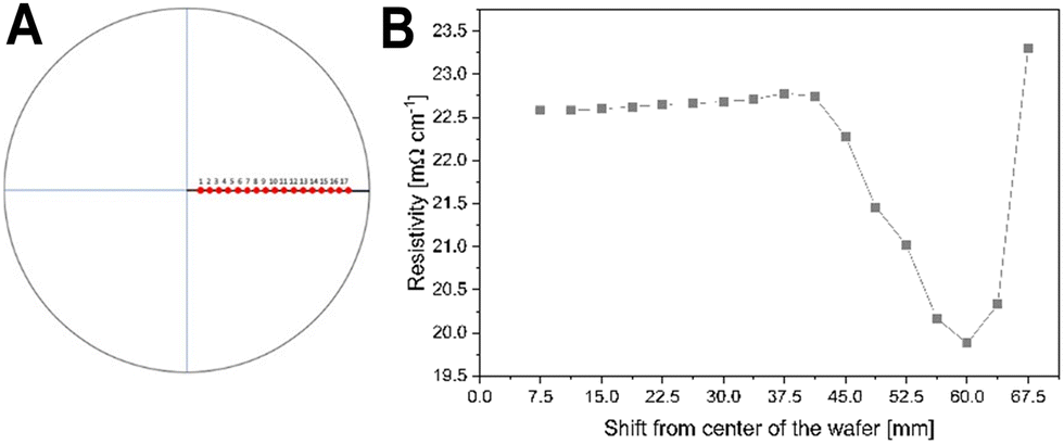Fig. 3 Eddy current measurement points (A) and resistivity value vs. position of the measurement in the wafer Pol 01 (B).

We developed a MLR regression model to correlate resistivity by Eddy current and 4 variables of the Raman spectrum on LOPC mode; using intensity and FWHM the RMSE in prediction is equal to ca. 0.80 mΩ cm, while the coefficient of determination R² is equal to ca. 0.96 both in cross-validation and in fitting (full values are reported in ESI†), leading to good performances both in description of the data employed to train it and at predicting the resistivity value for new, unknown samples. This model is written using R and making use of the caret framework⁴ to perform cross-validation; note that the data were previously autoscaled, i.e. the mean value of each predictor variable was subtracted from each value, and then they were divided by the standard deviation of each variable to remove any scaling effect, thus making them comparable. It should be pointed out that many different models were trained using various combinations of LOPC bands, including intensities, widths and even positions of their maxima, by applying the same procedure described above (MLR with cross-validation), to find the one with the best performances. In the end, the best model was the one just described, which does not consider the positions of the LOPC band, which contributes to an increase in the uncertainty in prediction, leading overall to worse performance.

Four single points were selected from the 17 measured points, chosen in the region where the resistivity values are constant for any wafer, to increase the level of statistical significance. In particular, the values at 11.25, 15.00, 18.75 and 22.50 along the Y-axis of measurement were used to calculate an average value. Fig. 4 illustrates that the predicted values are approximately aligned with the bisector of the plot, indicating a high degree of similarity with the observed (actual) resistivity values. Conversely, the residuals exhibit a uniform and random distribution, lacking any discernible trends. This observation suggests that the regression model is of satisfactory quality, free from any critical issues such as the omission of relevant factors or heteroscedasticity. This model allows us to convert the values associated with the variables of the LOPC band of the Raman spectra into resistivity values and to predict the resistivity within the linearity range between 12 and 25 mΩ cm.

Fig. 4 Score plot of observed vs. predicted resistivity values (A) and residual vs. predicted resistivity values (B).

In order to test the efficacy of this model, a comparison was conducted between the 17 Eddy current analysis points and the Raman analyses performed on the same points on a wafer that was excluded from the construction of the model (test set). The results demonstrated a prediction R² of 0.89 and an RMSE prediction error of 0.60 mΩ cm⁻¹. The Fig. 6 shows a good overlap of the predicted resistivity values, for higher values (between 19.5 and 20 mΩ cm⁻¹), while at lower values (between 18.5 and 17 mΩ cm⁻¹) the error is larger. The analysis point furthest from the centre of the wafer (point 17) shows a low prediction since it is located near the edge of the sample, whereas in this area the Eddy current technique shows low measurement precision.

3. Results and discussion

As seen above, it has been reported that the shape of the line and the peak frequency of the longitudinal optical phonon-plasmon coupled mode (LOPC) show noticeable changes when the carrier concentration in 4H-crystals SiC changes.¹² LOPC deconvolution band shows two bands respectively 838 and 964 cm⁻¹ here called p5 (axial mode) and P6 (planar mode); to evaluate the resistivity in SiC wafers, let's consider changes in band intensity, band position (shift) and full width half maximum (FWHM). In this instance, it is important to note that the intensity of the band under consideration is not taken as absolute; instead, it is relative in nature. This relative intensity is determined by the ratio between the band of interest and the FTO band at 784 cm⁻¹ (referred to as p3). The selection of the p3 band as the reference point is due to its status as the strongest band in the spectrum, with its intensity being constant. In fact, the FTO modes are not primarily sensitive to changes in resistivity because being structural in origin, do not directly correlate with changes in dopant concentration or free carrier densities that alter resistivity.²³ As an illustration, contemplate a slice of the polished sample (Polished wafer 01) from the production chain (Fig. 5). On the right side of the device, there is a dark area on the wafer surface, which, as reported by Zaho,²⁴ who discusses the impact of doping variations including colour changes, could indicate an inhomogeneity in the amount of nitrogen. The slice maps in Fig. 6 were created using 92 analysis points and are polished slices with a smooth and shiny surface. The values obtained from Raman analysis are reported in Table 2. Position and FWHM measurements are expressed in terms of difference from the reference value (Δ [cm⁻¹]) and intensity measurements are expressed as a ratio to other intensities (p3, more intense band) and are therefore pure numbers. Resistivity led to significant changes in the shape and position of the longitudinal optical phonon (LOPC)¹² and was attributed to changes in the peak position, spectral shape, and width. Resistivity is inversely related to free carrier concentration. As resistivity decreases (indicating higher carrier concentration), the LOPC band shifts to higher wavenumbers and broadens due to stronger plasmon–phonon coupling;²⁵ oppositely, higher resistivity causes a decrease in intensity and a shift towards lower wave numbers in this band, while also reducing the width of the FWHM parameter, which is marked by blue areas in maps.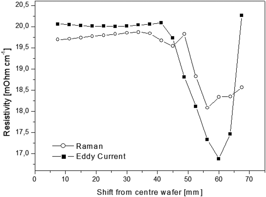

Fig. 5 Resistivity value vs. position of the measurement with Eddy current and Raman analysis in the wafer of the training set.

Fig. 6 Maps of SiC wafer polished 01 to evaluate resistivity, based on position, FWHM and intensity of p5 and p6 bands.

The regression model facilitates reasoning about resistivity variation because LOPC modes are associated with it. Currently, each wafer is associated with a single resistivity value obtained from a single eddy current analysis carried out on the central point of the wafer; the use of the linear regression model on the average of the four Raman analysis points closest to the wafer centre point showed similar resistivity values (Table 3). Raman analysis, through creating false colour maps (Fig. 7), reveals that resistivity is not uniform throughout the wafer. The variation detected in the samples is between roughly 1–2 (central blue and yellow areas) and 7–8 mΩ cm⁻¹ (blue areas). By way of example, in Fig. 7 we show a comparison between the map in false colour of three polished wafers (Pol 02-03-04), of expected resistivity, with that associated with the band p5, which turned out to be the most compatible. As you can see the intensity of the band p5 and resistivity show a direct correlation; further, the study also confirmed that resistivity values vary from wafer to wafer.

Table 3 Average resistivity measured with Eddy current vs. resistivity values predicted with the regression model

Wafer SiC	Resistivity mean [mΩ cm^−1]
	Eddy current	Raman
Pol 03	17.64	12.51
Pol 02	19.37	19.04
Pol 01	20.07	19.58

---

Fig. 7 The 92-point maps obtained with the linear regression model; p5 band intensity vs. predicted resistivity.

The resistivity with the Eddy current technique was measured only along the 4 collinear points, but through the regression model, it is possible to detect the resistivity on each point of the wafer with a non-contact Raman measurement. In addition, the measurement with Raman and the resistivity predicted by the MLR model provide a more accurate value; the false-colour maps allow us to make some considerations. For example, the Pol 02 wafer map shows a blue area on the right side where the resistivity values are lower (14–15 mΩ cm⁻¹ blue area) than the other areas (19–20 mΩ cm⁻¹ yellow area). In the area on the right, the upper side of the slice shows slightly lower resistivity than the lower half (17–18 mΩ cm⁻¹); this indicates a non-homogeneity of resistivity in different areas of the slice surface.

As an example, we have also reported the slice Pol 03 which shows, curiously, a marked inhomogeneity of the resistivity, higher along the circumference of the slice (yellow areas approximately 19–20 mOhm cm⁻¹) compared to the rest of the slice (blue areas approximately 12–13 mOhm cm⁻¹); moreover, this is the reason why this slice presents a large SD in the measurements (Table 3).

It is important to note that while the unit of measurement of the colour scale of the maps is relative to each individual map, as the parameters of each band vary individually, the scale of the predicted resistivity maps varies in the range of 12 to 25 mΩ cm⁻¹, which are the minimum and maximum values, respectively, detected at the samples under investigation. It was also observed that the resistivity changes concerning the side of the wafer; the investigation conducted on the two sides of the Pol 04 polished wafer (laser up/down) showed different behaviour for the p5 values of position intensity and FWHM within the 0.4-μm surface layer and variations in the layers between 0.4 and 4 μm below the surface (ESI,† Fig. S6).

As a result, the resistivity is both different and distributed differently on the two sides of the same wafer; Fig. 8 shows a comparison of the intensity p5 (Fig. 8(A) and (B)) and resistivity (Fig. 8(C) and (D)) value maps of the two sides of the Pol 03 wafer.

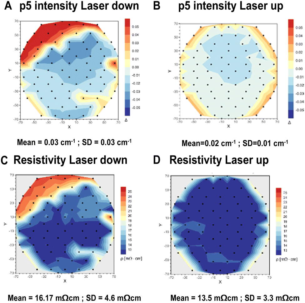Fig. 8 The 92-point maps of p5 intensity band of the two different sides of the polished wafer Pol 03 (down A and up B) vs. the predicted resistivity calculated with the linear regression model (down C and up D).

The predicted values of the resistivity and p5 band are in line with the behaviour of the LOPC region of the spectra recorded at different measurement depths. Specifically, analysis was carried out at five different depths, as previously explained in the Materials and methods section. This was achieved by varying the optical magnification of the microscope at two different points on the polished wafer Pol 03. The values of d_f and the corresponding resistivity, calculated using the model, are shown in Table 4.

Table 4 Optical magnification, the numerical aperture of the lens (NA), calculated depth of analysis along Z, and predicted resistivity, calculated using our model, for two points (1–8 and 5–2) on the polished wafer Pol 03

Optical magnification	NA	Depth of resolution (df) [μm]	Predicted resistivity point 1–8 [mΩ cm]	Predicted resistivity point 5–2 [mΩ cm]
100×	0.90	0.66	18.07	19.49
80×	0.75	0.95	17.99	19.81
50×	0.50	2.13	18.51	20.06
20×	0.40	3.32	18.49	20.70
10×	0.25	8.51	17.58	20.62

---

This technique allows monitoring along the Z-axis of the wafer; as expected, also in this case we obtain a variation of the resistivity values of about 1 mΩ cm at different depths, nonprogressive, from the surface to the bulk of the material. This demonstrates that the inhomogeneity of the resistivity is present in the three dimensions. The potential of the technique makes it a measure not only of the surface but also of depth and potentially allows us to investigate the bulk and to make predictions when the surface of the wafer is consumed/eroded. Furthermore, the method was employed exclusively for regions of the wafer comprising the 4H-SiC polytype, due to the fact that distinct polytypes (e.g. 6H or 15R) encompass additional bands, which precludes the applicability of our model. If resistivity varies along the thickness of the wafer, several problems may arise for the performance of electronic devices; a non-uniform distribution of resistivity can affect the internal electric fields causing an uneven distribution of the current through the material, reducing the efficiency and reliability of the device. Furthermore, a non-uniform distribution of resistivity can lower the breakdown voltage, a crucial parameter for high voltage applications. A non-homogeneity in resistivity could also lead to thermal management problems: inside SiC, known for its high thermal conductivity, essential for dissipating heat in power devices, a variability of resistivity can locally modify this property, creating hot spots and thermal instabilities generating localized overheating.^26,27

4. Conclusions

The research work undertaken has enabled relevant information to be obtained on SiC wafers. μRaman analysis combined with Eddy current measurements and the analysis of the data allows one, through pointwise analysis, to obtain information and to generate false-colour maps of resistivity, as evidenced by the change in the LOPC signal between 838 and 964 cm⁻¹. Using those components, it was possible to obtain information about the distribution of resistivity in the wafers in the form of false-colour images. Through the development of a resistivity calibration line related to a specific component of the μRaman spectrum, it was possible to create false-colour resistivity maps of individual wafers, in which each mapped point is assigned a resistivity value. Relevant R-language codes have been generated that allow the automation of the curve fitting of the obtained spectra, for the automatic generation of false-colour images for each individual wafer analysed. The false-colour maps confirm the inhomogeneity of resistivity in the wafers, and transform these variations into a numerical value of resistivity per cm, in the range between 12 to 25 mΩ cm. The variation in resistivity was also observed in the bulk of the slices; in fact, opposite sides of the same slice show different resistivity values, distributed non-uniformly along the Z axis. It is important to be able to diagnose these discrepancies to quickly and accurately evaluate the non-conformity of these devices; finally, all this information is gathered through a single μRaman analysis of the wafer, which is a non-contact analysis, thus allowing the measured surface area of the wafers not to be altered. It is imperative to acknowledge the limitations of the model and the conclusions drawn by the authors. The validity of the model is constrained to the experimental analysis conditions utilised, namely the wavelength and power of the selected laser, the analysis time, and the room working temperature (25 °C). Subsequent investigations may be conducted in the future to expand the parameters, encompassing variations in laser type and power, as well as different working temperatures. Indeed, the present method may be subject to restrictions due to the possibility of hopping transport (which is dominant at low temperatures),²⁸ and further studies are required to explore this possibility, although these are outside the scope of the present paper.

Author contributions

Elisa Calà – Simone Cerruti: data curation, formal analysis, investigation, original draft preparation and writing. Cristina Sanna – Marco Maffè: conceptualization, sample collection, visualization and investigation. Wen Chin Hsud – Man Hsuan Lind: conceptualization, visualization and sample collection. Luciano Ramello – Giorgio Gatti: conceptualization, supervision, reviewing and editing.

Data availability

A data availability statement is provided herewith. The data supporting this study, including Raman spectra and ADE Eddy current analysis, are obtained from commercial materials and, as a consequence of the restrictions imposed by the relevant commercial parties, cannot be made available. The code for creating the model using the R² Statistic software has been included as part of the ESI.†

Conflicts of interest

The authors declare no competing interests.

Acknowledgements

This work was financially supported by GlobalWafers Co., Ltd No. 8, Industry E. Rd. II, Hsinchu Science Park, Hsinchu 30075, Taiwan, and MEMC Electronic Materials Spa, A GlobalWafers Company – Viale Luigi Gherzi 31, 28100 Novara (NO), Italy that provided the samples.

Notes and references

1. X. She, A. Q. Huang, Ó. Lucía and B. Ozpineci, Review of Silicon Carbide Power Devices and Their Applications, IEEE Trans. Ind. Electron., 2017, 64(10), 8193–8205,  DOI:10.1109/TIE.2017.2652401.
2. R. Gerhardt, Properties and applications of Silicon Carbide, In Tech, Rijeka (Croatia), 2011.
3. Z. Xu, Z. He and Y. Song, Application of Raman Spectroscopy Characterization in Micro/Nano-Machining, Micromachines, 2018, 9(7), 361.
4. K. Muthuramalingam and W.-C. Wang, Non-destructive mapping of electrical properties of semi-insulating compound semiconductor wafers using terahertz time-domain spectroscopy, Mater. Sci. Semicond. Process., 2024, 170, 107932.
5. R. Dalmau, S. Kirby, J. Britt and R. Schlesser, Mapping Analysis of Crystalline Perfection and UV-C Transparency of 2-in. Aluminum Nitride Substrates Grown by Physical Vapor Transport, Phys. Status Solidi B, 2023, 2300482.
6. J. Boguski, J. Wróbel, S. Złotnik, B. Budner, M. Liszewska, Ł. Kubiszyn, P. P. Michałowski, Ł. Ciura, P. Moszczyński, S. Odrzywolski, B. Jankiewicz and J. Wróbel, Multi-technique characterisation of InAs-on-GaAs wafers with circular defect pattern, Opto-Electron. Rev., 2023, 31, e144564.
7. Q. Xu, N. Yu and F. Essaf, Improved Wafer Map Inspection Using Attention Mechanism and Cosine Normalization, Machines, 2022, 10, 146.
8. J. Koo and S. Hwang, A Unified defect pattern analysis method based on density-based clustering (DBC), IEEE Access, 2021, 9, 78873.
9. D. M. A. MacKenzie, K. G. Kalhauge, P. R. Whelan, F. W. Stergaard, I. Pasternak, W. Strupinski, P. Bøggild, P. U. Jepsen and D. H. Petersen, Wafer-scale graphene quality assessment using micro four-point probe mapping, Nanotechnology, 2020, 31, 225709.
10. Y.-C. Tseng, Using Visible Laser-Based Raman Spectroscopy to Identify the Surface Polarity of Silicon Carbide, J. Phys. Chem., 2016, 120, 18228–18234.
11. Z. M. Wang, One-Dimensional Nanostructures, Springer, New York., U.S., 2008.
12. S. Nakashima and H. Harima, Raman investigation of SiC polytypes, Phys. Status Solidi A, 1997, 162(1), 39–64.
13. J. C. Burton, et al., Spatial characterization of doped SiC wafers by Raman spectroscopy, J. Appl. Phys., 1998, 84(11), 6268–6273.
14. T. Liu, Z. Xu, M. Rommel, H. Wang, Y. Song, Y. Wang and F. Fang, Raman Characterization of Carrier Concentrations of Al-implanted 4H-SiC with Low Carrier Concentration by Photo-Generated Carrier Effect, Crystals, 2019, 9, 428,  DOI:10.3390/cryst9080428.
15. A. Meli, A. Muoio, A. Trotta, L. Meda, M. Parisi and F. La Via, Epitaxial Growth and Characterization of 4H-SiC for Neutron Detection Applications, Materials, 2021, 14, 976.
16. H. Harima, S. Nakashima and T. Uemura, J. Appl. Phys., 1995, 78, 1996.
17. S. Nakashima and K. Tahara, Phys. Rev., 1989, 6339, B40.
18. H. Harima, Raman scattering characterization on SiC, Microelectron. Eng., 2006, 83, 126–129.
19. M. Kuhn, Building Predictive Models in R Using the caret Package, J. Stat. Softw., 2008, 28(5), 1–26.
20. M. Born and E. Wolf, Principle of Optics: Electromagnetic Theory of Propagation, Interference and Diffraction of Light, Cambridge University Press, Cambridge, UK, 7th edn, 1999.
21. J. Yang, S. Huaping, J. Jikang, W. Wenjun and C. Xiaolong, Characterization of morphological defects related to micropipes in 4H-SiC thick homoepitaxial layers, J. Cryst. Growth, 2021, 568–569, 126182.
22. G. Wandong, Y. G. Guang, Y. Qian, X. Han, C. Cui, X. Pi, D. Yang and R. Wang, Dislocation-related leakage-current paths of 4H silicon carbide, Sec. Semiconducting Materials and Devices Front. Mater., 2023, vol. 10 DOI:10.3389/fmats.2023.1022878.
23. S. Nakashima, H. Katahama, Y. Nakakura and A. Mitsuishi, Relative Raman intensities of the folded modes in SiC polytypes, Phys. Rev. B: Condens. Matter Mater. Phys., 1986, 33(8), 5721–5729.
24. L. Zaho, Surface defects in 4H-SiC homoepitaxial layers, Nanotechnol. Precis. Eng., 2020, 3, 229–234,  DOI:10.1016/j.npe.2020.12.001.
25. Y. Song, Z. Xu, T. Liu, M. Rommel, H. Wang, Y. Wang and F. Fang, Depth Profiling of Ion-Implanted 4H–SiC Using Confocal Raman Spectroscopy, Crystals, 2020, 10(2), 131,  DOI:10.3390/cryst10020131.
26. D. A. Gajewski, B. Hull, D. J. Lichtenwalner, S. Ryu, E. Bonelli and H. Mustain, SiC power device reliability, SiC power device reliability, 2016 IEEE International Integrated Reliability Workshop (IIRW), South Lake Tahoe, CA, USA, 2016, pp. 29–34 DOI:10.1109/IIRW.2016.7904895.
27. M. Östling, R. Ghandi and C.-M. Zetterling, “SiC power devices – Present status, applications and future perspective,” 2011 IEEE 23rd International Symposium on Power Semiconductor Devices and ICs, San Diego, CA, USA, 2011, pp. 10–15 DOI:10.1109/ISPSD.2011.5890778.
28. H. Hergert, M. T. Elm and P. J. Klar, Validation of Raman spectroscopy as a tool for mapping transport parameters in inhomogeneous N-doped 4H-SiC, J. Raman Spectrosc., 2023, 54(7), 737–747,  DOI:10.1002/jrs.6531.

---

Footnote

† Electronic supplementary information (ESI) available. See DOI: https://doi.org/10.1039/d4cp04545a

---