Resolving the effect of roadside vegetation barriers as a near-road air pollution mitigation strategy†
Received
4th August 2023
, Accepted 10th January 2024
First published on 18th January 2024
Abstract
Communities located in near-road environments experience elevated levels of traffic-related air pollution. Near-road air pollution is a major public health concern, and an environmental justice issue. Roadside green infrastructure such as trees, hedges, and bushes may help reduce pollution levels through enhanced deposition and mixing. Gaussian-based dispersion models are widely used by policymakers to evaluate mitigation strategies and develop regulatory actions. However, vegetation barriers are not included in those models, hindering air quality improvement at the community level. The main modeling challenge is the complexity of the deposition and mixing process within and downwind of the vegetation barrier. We propose a novel multi-regime Gaussian-based model that describes the parameters of the standard Gaussian equations in each regime to account for the physical mechanisms by which the vegetation barrier deposits and disperses pollutants. The four regimes include vegetation, a downwind wake, a transition, and a recovery zone. For each regime, we fit the relevant Gaussian plume equation parameters as a function of the vegetation properties and the local wind speed. Furthermore, the model captures particle deposition, a major factor in pollutant reduction by vegetation barriers. We parameterized the multi-regime model using data generated from a fields-validated computational fluid dynamics (CFD) model, covering a wide range of vegetation properties and meteorological conditions. The proposed multi-regime Gaussian-based model was evaluated across 9 particle sizes and a tracer gas to assess its capability of capturing dispersion and deposition. The multi-regime model's normalized mean error (NME) ranged between 0.18 and 0.3, the fractional bias (FB) ranged between −0.12 and 0.09, and R2 value ranged from 0.47 to 0.75 across all particle sizes and the tracer gas for ground level concentrations, which are within acceptable ranges for air quality dispersion modeling. Even though the multi-regime model is parameterized for coniferous trees, our sensitivity study indicates that it can provide useful predictions for hedges/bushes vegetative barriers as well.
Environmental significance
Around 45 million people live within 100 m of major roadways in the U.S. alone. Communities located in near-road environments experience elevated levels of traffic-related air pollution, which makes it a major public health concern and an environmental justice issue. Roadside vegetation barriers such as trees, hedges, and bushes reduce pollution levels through enhanced deposition and mixing. However, there are no tools suitable for regulators and communities to assess the effectiveness of pollutant reduction by vegetation barriers. We present a novel multi-regime framework to resolve the physical mechanisms in a computationally efficient, Gaussian-based model. The model evaluation shows its performance is within acceptable ranges for dispersion modeling and can be adapted into the regulatory modeling system for wide adoption.
|
1. Introduction
In communities near large roadways, people can be exposed to elevated traffic-related air pollution (TRAP) as they live, work and attend school. Exposures to TRAP have been associated with numerous adverse health effects including heart and respiratory diseases and premature mortality.1 In the U.S., an estimated 45 million people live and around 3.2 million students attend school within 100 m of major roadways,2,3 with many more communities at risk worldwide. Furthermore, people of low income and ethnic minority suffer disproportionately from exposure to TRAP.4,5 In summary, near-road air pollution is a major public health concern, and an environmental justice issue.
Roadside vegetation has been shown to be an option to help alleviate the health burden and mitigate near-road air pollution.6–8 The effectiveness of vegetation barriers to mitigate TRAP depends on many factors such as vegetation properties (size and density) and local urban conditions.9–12 Field measurements13,14 or computational fluid dynamics (CFD) modeling15,16 can be used to evaluate the effectiveness of pollutant reduction by vegetation barriers. However, local communities often lack the technical expertise and resources to perform field measurements or computationally intensive model simulations. A recent study demonstrated the potential of using machine learning tools to create a cloud-based design tool for roadside vegetation barrier designs.17 While the machine learning approach is very resource-efficient to the users, it provides little insight into the physical mechanisms by which the vegetation barriers affect air pollutants. Furthermore, it is challenging to integrate the machine learning model into existing regulatory models making them inaccessible to regulators and decision makers as they aim to find evaluation tools to assess the impact of roadside vegetation on pollutant reduction.
Widely used for regulatory and human exposure assessment purposes, Gaussian-based dispersion models provide mathematical descriptions of pollutant transport in the atmosphere. Those models describe the statistical behaviors of diffusion and advection, and incorporate parameterization schemes, developed using wind tunnels18 and field measurement data.19 Previous studies have proposed formulations within the Gaussian modeling framework to account for the influence of roadside solid barriers on pollutant dispersion.20–22
However, incorporating the effect of roadside vegetation barriers into the Gaussian modeling framework is much more complex than solid barriers for multiple reasons. First, unlike solid barriers, the physical mechanisms by which vegetation barriers affect pollution dispersion depend on the barriers' porosity. Second, pollutants can deposit on the leaves of vegetation, resulting in pollutant reduction so the effect of deposition needs to be properly described. Third, there is a lack of high-resolution spatial pollutant concentration datasets, making it challenging to develop such a model. To the best of our knowledge, there are no studies that have developed a dispersion model to characterize pollutant concentrations downwind of vegetation barriers.
We propose a multi-regime approach to parameterize the Gaussian plume equations to describe the dispersion and deposition of air pollutants for roadside vegetation barriers. To the best of our knowledge, this is the first time that the effect of roadside vegetation barriers has been incorporated into a Gaussian-based dispersion model, which then enables potential future integration into the existing regulatory models providing policymakers and communities with a tool to assess vegetation barriers designs and their impact on pollutant reduction. This tool can be used to generate effective urban green designs that mitigate TRAP for many local communities in dire need of improvements in local air quality.
The proposed model captures the physical mechanisms by defining four regimes within and downwind of the vegetation. In each regime, the Gaussian plume equation parameters are characterized as a function of the vegetation properties and wind speed. We conducted 75 high-fidelity CFD simulations, using the Comprehensive Turbulent Aerosol Dynamics and Gas Chemistry (CTAG) model, to train and test the proposed parameterized Gaussian-based model. Those simulations covered a wide range of vegetation barriers and wind speeds; in addition, the CTAG model has been validated against various field measurement studies to ensure that it can properly capture both the aerodynamic and deposition impacts of the vegetation barrier.
This paper is organized as follows. Section 2 describes the CTAG model and computational domain. Section 3 discusses the proposed multi-regime approach and the steps to parameterize the Gaussian equations. Section 4 assesses the performance of the parameterized Gaussian-based model and discusses its limitations. Finally, Section 5 highlights the conclusions of this study.
2. Methods
2.1 The CTAG model and simulations
2.1.1 Vegetation representation.
This study focused on coniferous vegetation since this species generally does not lose its leaves in the winter, hence experiences little seasonal impact, and is dense close to ground level, which are important characteristics to mitigate TRAP. There are two parameters characterizing the vegetation density, i.e., leaf area density (LAD) and leaf area index (LAI). The LAD describes the leaves surface area per unit volume within the vegetation and is used to evaluate the vegetation drag on the flow, and particle deposition on the vegetation as highlighted in the following sections. The LAD profile for conifers vegetation was used following eqn (1):23| |  | (1) |
Lm is the maximum LAD within the vegetation, z is the height, zm is the height at which Lm occurs (zm = 0.4 h), h is the vegetation height, and n is a fit parameter. LAI measures the projected area of leaves per ground surface area. If the LAI value and LAD profile are known, Lm can be obtained using eqn (2).| |  | (2) |
2.1.2 CTAG: model, computational domain and boundary conditions.
The CTAG model is designed to resolve the flow field including turbulent reacting flows, aerosol dynamics, and gas chemistry in complex environments.24–26 In this paper, we employed the Large Eddy Simulation (LES) model to resolve the flow and turbulence. The semi-implicit method for pressure linked equation (SIMPLE) algorithm was used to couple the velocity–pressure equations, and a second-order upwind discretization scheme was used for the momentum and scalar transport equations. For the LES simulations, the dynamic Smagorinsky model was implemented to account for the subgrid turbulent viscosity.27 The CTAG model is described in more detail in Section 2.1.4.
Fig. 1 displays a vertical and top view of the CTAG computational domain, which we employ to generate training data to develop the parameterized Gaussian-based model. The domain dimensions were 60 m in the vertical direction, 60 m along the driving direction, and 250 in the spanwise direction. Two zones, of height 3 m and width 14 m, were used to represent emission sources from two-way traffic. Two other zones were used to represent two rows of vegetation. The vegetative barrier was implemented as close as possible to the highway, with a 5 m distance between the traffic zone and the vegetative barrier, to account for the highway shoulder designated for emergency use. In addition, the vegetative barrier spanned the total width of the domain to describe an infinitely long barrier. The domain consisted of 7.5 million cells with uniform mesh of sizing 0.492 m. Fig. S1 in the ESI† shows a side view of the mesh that was uniform. A mesh sensitivity study, with a mesh of 0.38 m and a total of 14.7 million cells, showed little difference compared to the original mesh, indicating that it accounts for the turbulent kinetic energy (TKE) produced in the domain (Fig. S2†). The applied boundary conditions were a neutral atmospheric boundary layer (NABL) velocity profile at the inlet,28 pressure outflow at the outlet, and symmetry boundary conditions for the top of the domain and the sides, thus simulating an infinitely long barrier. Details on the applied NABL at the inlet are provided in Section S1 of the ESI.†
 |
| | Fig. 1 A sketch of the CTAG computational domain used in this study (a) top view; (b) side view. | |
2.1.3 CTAG-generated dataset.
We employed the CTAG model to generate data that reflected a wide range of applicable vegetative barriers and urban conditions. The explored height range of vegetative barriers varied from 2 to 10 m. The width to height ratio of the vegetation was 2![[thin space (1/6-em)]](https://www.rsc.org/images/entities/char_2009.gif) :
:![[thin space (1/6-em)]](https://www.rsc.org/images/entities/char_2009.gif) 3, which represents coniferous vegetation, and was used in previous studies.29,30 The vegetation barrier consisted of two rows of vegetation to ensure that it had no gaps in it; therefore, the barrier's width to height ratio was 4
3, which represents coniferous vegetation, and was used in previous studies.29,30 The vegetation barrier consisted of two rows of vegetation to ensure that it had no gaps in it; therefore, the barrier's width to height ratio was 4![[thin space (1/6-em)]](https://www.rsc.org/images/entities/char_2009.gif) :
:![[thin space (1/6-em)]](https://www.rsc.org/images/entities/char_2009.gif) 3. In addition, we explored three LAI values 4, 7, and 11 to reflect various vegetation density values which account for a wide range of vegetation (Asner et al., 2003). Different urban conditions were considered by covering a range of velocities from 1 to 5 ms−1 at a height of 10 m. In total, we simulated 75 cases which highlighted 5 different barrier heights, 5 different velocities, and three different LAI values as shown in Table 1. The 75 CTAG-generated cases were randomly split into 60 cases to train the parameterized Gaussian-based model, and 15 cases to test it representing an 80/20% split. The test cases were not used in any training to ensure rigorous evaluations. In addition to the 75 cases, we simulated 5 other cases with no barrier at five different wind speeds to normalize the results and understand the impact of the barrier compared to no vegetation.
3. In addition, we explored three LAI values 4, 7, and 11 to reflect various vegetation density values which account for a wide range of vegetation (Asner et al., 2003). Different urban conditions were considered by covering a range of velocities from 1 to 5 ms−1 at a height of 10 m. In total, we simulated 75 cases which highlighted 5 different barrier heights, 5 different velocities, and three different LAI values as shown in Table 1. The 75 CTAG-generated cases were randomly split into 60 cases to train the parameterized Gaussian-based model, and 15 cases to test it representing an 80/20% split. The test cases were not used in any training to ensure rigorous evaluations. In addition to the 75 cases, we simulated 5 other cases with no barrier at five different wind speeds to normalize the results and understand the impact of the barrier compared to no vegetation.
Table 1 Vegetation properties of the various barriers explored in this study
| H (m) |
W (m) |
LAI = 11 |
LAI = 7 |
LAI = 4 |
|
L
m (m−1) |
L
m (m−1) |
L
m (m−1) |
| 2 |
2.5 |
7.5 |
4.81 |
2.75 |
| 4 |
5 |
3.75 |
2.4 |
1.38 |
| 6 |
8 |
2.5 |
1.6 |
0.92 |
| 8 |
10.5 |
1.88 |
1.2 |
0.69 |
| 10 |
13 |
1.5 |
0.96 |
0.55 |
2.1.4 Vegetation drag and size-resolved particle deposition in CTAG.
Since it is computationally prohibitive to explicitly model the vegetation elements, such as leaves and branches, the effects of vegetation were spatially averaged and included as source terms in the governing equations.31 The drag induced by vegetation is accounted for by including a sink term to the momentum equations:32where Si is the sink term, Cd (=0.3) is the plant drag coefficient, LAD(z) is the LAD profile, U is the velocity magnitude of the flow, and ui is the velocity in the direction of interest.
We simulated 9 different particle sizes that ranged from 15 to 253 nm, to account for traffic exhaust emissions.13 The particle sizes are small, so they are assumed to trace the fluid flow. In addition, we simulated a tracer gas that does not experience deposition to isolate the effects of barrier on pollutant dispersion. To model the particle dispersion, a scalar transport equation was used, and a sink term was included to account for deposition (eqn (4)).
| | Sd(Dp) = ρVd(Dp)Np(![[D with combining tilde]](https://www.rsc.org/images/entities/i_char_0044_0303.gif) p)LAD(z) p)LAD(z) | (4) |
where
Np(
![[D with combining tilde]](https://www.rsc.org/images/entities/i_char_0044_0303.gif) p
p) is the average particle concentration of a particle size
Dp, and
Vd(
Dp) is the deposition velocity adopted from a widely used dry deposition model.
33 To assess if the proposed multi-regime parametrized Gaussian-based model captured the deposition and dispersion of the vegetation barrier, the performance for each of the 9 particle sizes and the tracer gas is provided. The governing equations for momentum, dispersion, and deposition are included in Section S2 of the ESI.
† The CTAG model highlighted in this section aligns with those used in our previous studies.
10,11,15
2.1.5. CTAG model evaluation.
Tong et al.15 assessed the CTAG model against field measurements conducted by Hagler et al.13 Those measurements included ultrafine particle size distributions (PSD) which were collected behind a near-road barrier consisting of 6–8 m tall conifer vegetation. The CTAG model showed good agreement with the PSD from the field measurements, indicating that it captures deposition on the vegetative surfaces. Hashad et al.11 also evaluated the aerodynamic performance of the CTAG model by comparing the mean velocity and Reynold stress to that obtained by field measurements in a maize canopy,34 highlighting good performance by the CTAG model.
3. A multi-regime approach to parameterize Gaussian-based plume equations
The purpose of our study was to try to parameterize the Gaussian-based plume equations to describe how the pollutant concentration decays downwind of a vegetative barrier. To do so, we propose a multi-regime approach based on the physical mechanisms by which the barrier disperses pollutants. The overall goal was to use variables such as the vegetation properties (dimensions and density) and local wind speed conditions to characterize the Gaussian plume parameters.
3.1. Gaussian plume equations
Gaussian plume dispersion models have been widely used to describe pollutant dispersion in various atmospheric conditions. Our study focuses on an infinitely long emission source and vegetation barrier. The Gaussian plume equation for an infinitely long emission source, where the concentration is horizontally uniform, and only a function of the downwind distance (x) and vertical height (z), can be obtained using eqn (5).| |  | (5) |
where A is the emission rate, U is the plume velocity, zs is the source height, and σz is the vertical plume spread defined as one third of the plume width, i.e., the distance from the ground to edge of the plume that has the lowest concentration. One third was chosen since the vertical spread σz also denotes the standard deviation of the Gaussian distribution, and 99.73% of the plume concentration falls within 3 standard deviations. The plume velocity was evaluated using the mass weighted plume velocity described by eqn (6):| |  | (6) |
where h is the height of the plume, C is the spatial concentration, and u(z) is the velocity at different heights.
3.2. Multi-regime approach
The vegetation barrier affects the fluid flow within and around the barrier, influencing both particle deposition and dispersion. By analyzing the physics of the flow induced by the barrier, we can determine characteristic regimes to parameterize the flow. Using a single-regime model is challenging. For example, the behavior of the mean plume velocity behind the barrier is highly non-linear (Fig. 5a) and difficult to parameterize within a unifying set of equations. By contrast, a multi-regime approach allows separate parameterization in each regime. Fig. 2 shows the four regimes of the proposed parametrized Gaussian-based model which were based on the flow characteristics. Regime I is located within the vegetation where leaves induce drag on the flow and particles deposit on the vegetation, and its length corresponds to the vegetation barrier's width. Regime II is the vegetation wake, which is characterized by low velocity and turbulence, resulting in reduced pollutant dispersion, and its length depends on the vegetation properties and was parameterized as highlighted in Section 3.5. Regime III is a transition regime where there is high turbulence, and velocity recirculation for some cases (Fig. 2). The simulation results suggest that the extent of the transition zone could be approximated as three barrier heights (3H) to simplify the model. Finally, in regime IV the TKE produced by the barrier starts decaying and the velocity starts to recover to the NABL profile. Furthermore, the influence of the turbulence, generated by the barrier, spans a height of approximately 2.2H which will affect pollutant dispersion. By identifying those zones, the behavior of the different Gaussian parameters can be analyzed and fitted for each zone.
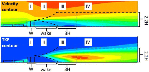 |
| | Fig. 2 The multi-regime approach is defined by four different regimes which include the vegetation, wake, transition, and recovery zones. | |
3.3. Overview of the multi-regime parameterized Gaussian-based model
Fig. 3 illustrates the overall model development process, which aims to use easily obtained input features, to describe the relevant parameters of the proposed model in each zone identified in the multi-regime description. The user input consists of five main features: Wind speed at height 10 m (U10), vegetation barrier height (H), width (W), LAI, and maximum LAD, Lm. There are 5 key parameters that need to be parameterized: One spatial parameter (wake length, lwake), and 4 relevant parameters of the Gaussian plume equations that include U, σz, A, and zs. Note that the emission source rate, A, was parameterized in order to account for particle deposition by the barrier, and the source height, zs, to account for potential changes in the plume peak location due to the vegetation.
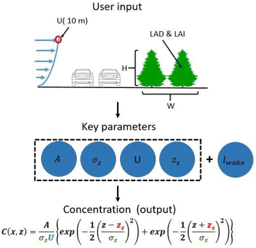 |
| | Fig. 3 The parametrized Gaussian-based model aims to use simple user input to evaluate the key parameters and use them to obtain the pollutant concentration using the Gaussian plume equations. | |
3.4. Parameterization process
Fig. 4 depicts the parameterization steps. The Gaussian equation parameters of interest were first obtained from the simulated training cases and analyzed in each of the four regimes of the proposed parametrized Gaussian-based model. Then, based on the behavior of the parameter in each regime, either a constant, linear, or quadratic fit was used to describe that parameter. The slope of the linear and quadratic parameterization was then fitted as a function of the five features including the vegetation properties and velocity. To perform the fitting for the slopes of interest, an iterative process was followed. First, the slope was fitted as a function of each of the five main features. Then, the feature with the best fit, determined by the highest R2, was used to normalize the slope. After that, the normalized slope was described as a function of the remaining features by repeating the same fitting process. This process stopped when the R2 of the fit was less than 0.2 which indicates that the fit was almost independent of the remaining features and also ensured the parametrized Gaussian-based model did not become overly complex. A detailed example of this fitting process is provided in Section S3 of the ESI.† The following sections present the parameterization for each parameter.
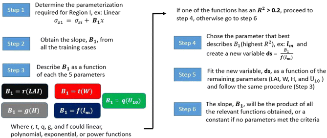 |
| | Fig. 4 The steps involved in parameterizing the key parameters of the Gaussian plume equations in each of the regimes of the parametrized Gaussian-based model. | |
3.4.1 Wake length, lwake.
The length of the wake regime will depend on the vegetation properties. From the CTAG simulations, the length of the wake regime was evaluated and then fitted as a function of the vegetation characteristics. Eqn (7) shows the parameterized equation that describes lwake as a function of the vegetation height, width, and density (Lm). Velocity did not strongly influence the wake length as highlighted in Section S4 in the ESI and Fig. S5.†| | | lwake = (3.03W−2.086 + 0.1042) (39Lm−0.7284)H | (7) |
3.4.2 Source height, zs.
The highest concentration occurs at the source height (z = zs). Dispersion models that describe the plume characteristics behind solid barriers, sometimes involve a source-shift such that the maximum concentration occurs at barrier height (zs = H).20 This accounts for the plume being vertically displaced upwards since the solid barrier is impermeable and forces the flow to go around it. Vegetation is a porous medium, so a large portion of the plume goes through it. We assumed that there was no source shift, in other words, the source height was assumed to be zero (zs = 0) in each zone, which indicates that the maximum concentration occurred at ground level, which agrees with the observed data (Fig. S6†). This produced favorable results, as highlighted in the results section. We also explored another model that assumes a source height shift that occurs in regime III and slowly decays in regime IV. However, the original model with no source shift performed better. A source shift can capture the behavior for certain cases that reflect very dense vegetation, which is highlighted in Section S5 of the ESI.† In those cases, the turbulence and recirculation generated in regimes III and IV were strong, causing the concentration to be well-mixed and almost uniform with respect to height, and then slowly recovered to ground level further downwind in regime IV. It is important to note that even for those cases, the proposed parametrized Gaussian-based model with no source shift also produces favorable results (Section S5†).
3.4.3 Mean velocity, U.
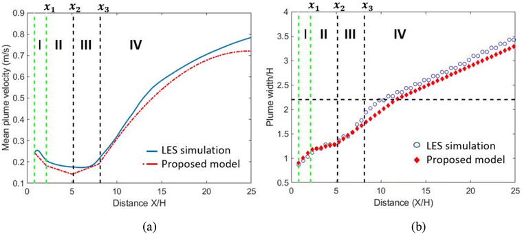
The mean velocity fitted for use in the multi-regime parametrized Gaussian-based model was obtained by calculating the plume-weighted mean velocity from the CTAG simulations using eqn (6). Fig. 5a shows the mean plume velocity for one of the training cases. The velocity decreased in regime I due to drag, then it further reduced in regime II (wake). In regime III, due to recirculation, the velocity reached a minimum before slowly recovering in regime IV. A linear fitting was chosen for regimes I, II, and III and a power fit was used for regime IV. The power fit in regime IV accounted for the mean plume velocity that will form an asymptote to the upstream velocity further downwind of the barrier. Fig. 5a highlights the proposed fitting, while eqn (8)–(11) show the functions that were used for each regime.| | U1 = Ui + C1(x), where![[thin space (1/6-em)]](https://www.rsc.org/images/entities/char_2009.gif) C1 = 0.022Lm−1.231 − 0.0149 C1 = 0.022Lm−1.231 − 0.0149 | (8) |
| | U2(x) = U1(x1) + C2(x − x1), where![[thin space (1/6-em)]](https://www.rsc.org/images/entities/char_2009.gif) C2 = (0.089Lm + 0.8) (−0.002U10) C2 = (0.089Lm + 0.8) (−0.002U10) | (9) |
| | U3(x) = U2(x2) + C3(x − x2), where![[thin space (1/6-em)]](https://www.rsc.org/images/entities/char_2009.gif) C3 = (0.003LAI − 0.008) (0.44U10 − 0.33) C3 = (0.003LAI − 0.008) (0.44U10 − 0.33) | (10) |
U4(x) = U3(x3) + C4(x − x3)C5, where![[thin space (1/6-em)]](https://www.rsc.org/images/entities/char_2009.gif) C4 = (−0.44Lm−1.82 + 1.19) (0.054U10 − 0.016), C4 = (−0.44Lm−1.82 + 1.19) (0.054U10 − 0.016), |
| | | C5 = (0.13Lm−2.11 + 0.49) (0.36U10−18.68 + 0.96) | (11) |
x1,x2, and x3, are the locations of the boundaries between the different regimes, and since the fitting needed to be continuous, the value of the mean plume velocity is the same at those locations. The values of the fitting constants C1 to C5 were obtained for each of the training cases and fitted as a function of the vegetation properties and local wind speed following the fitting procedure highlighted earlier. The initial velocity, Ui, can be approximated as the velocity at the mid-plume height at the start of the vegetation.
 |
| | Fig. 5 (a) Mean plume velocity and (b) normalized plume width versus distance across the four regimes of the multi-regime approach for one of the training cases obtained from the LES simulation as well as the proposed fit of the multi-regime approach. | |
3.4.4 Vertical plume spread, σz.
Fig. 5b shows the plume width (3 times the vertical spread, σz) for one of the training cases. The plume spread increases strongly within the vegetation; as the flow slowed down due to drag, it expanded in the vertical direction thus advecting the plume with it. In regime II, the plume spread growth rate decreased as the wake was characterized by low turbulence and velocity, hence there was no effective mechanism to disperse pollutants. In regime III, the plume width experienced an increase as a result of the turbulence and recirculation in the transition zone. That growth was maintained until the plume exited the high TKE regime which extended to approximately to a height of 2.2H. After the plume exited that regime, the effects of the vegetation became minimal, and the plume growth was predominantly dominated by the local atmospheric conditions.
We used a linear fitting for each of the four regimes as it described the plume spread growth well, while keeping the parametrized Gaussian-based model simple as highlighted in Fig. 5b and eqn (12)–(15). Since the turbulence-related effects of the barrier on the plume are dominant up to a height of 2.2H, the fitting only applies to that height range. After the plume exits that regime, (plume width >2.2H) the plume growth is dictated by the local atmospheric conditions and equations that describe the vertical dispersion for near surface source can be used:35–37
| | σz1(x) = σzi + B1(x), where![[thin space (1/6-em)]](https://www.rsc.org/images/entities/char_2009.gif) B1 = 0.037H−1.505 + 0.07 B1 = 0.037H−1.505 + 0.07 | (12) |
| | σz1(x) = σz1(x1) + B2(x − x1), where![[thin space (1/6-em)]](https://www.rsc.org/images/entities/char_2009.gif) B2 = 0.013 B2 = 0.013 | (13) |
| | σz3(x) = σz2(x2) + B3(x − x2), where![[thin space (1/6-em)]](https://www.rsc.org/images/entities/char_2009.gif) B3 = (6.95 × 10⁻⁴)H × LAI B3 = (6.95 × 10⁻⁴)H × LAI | (14) |
| | σz4(x) = σz4(x3) + B3(x − x3), where![[thin space (1/6-em)]](https://www.rsc.org/images/entities/char_2009.gif) B4 = (6.95 × 10⁻⁴)H × LAI B4 = (6.95 × 10⁻⁴)H × LAI | (15) |
The initial vertical spread, σzi, is integral as it provides the starting point for fitting the parametrized Gaussian-based model. Studies for near-surface source releases can describe the vertical dispersion for plumes in roadway settings with no roadside barriers. The presence of roadside vegetation will cause the incoming plume to expand because the flow slows due to the drag imposed on it. By evaluating the plume width for no barriers against that with roadside vegetation, we were able to obtain the following equation to account for the increase in plume width at the start of the vegetation and obtain the initial vertical spread,
| | | σzi = σa (0.042H + 1.118) (0.02873LAI + 0.7883) | (16) |
where
σa is the vertical dispersion obtained for near-source release applications with no roadside barriers.
3.4.5 Emission source, A.
Particles deposit on leaves as the plume passes through the vegetation canopy. To incorporate particle deposition in the multi-regime parametrized Gaussian-based model, the emission source term in the Gaussian equations needs to be modified, otherwise the model will overestimate pollutant concentration downwind of the barrier. To account for particle deposition, a mass balance was conducted before and after the vegetation to evaluate the particle reduction due to deposition for each of the training cases. When fitting the concentration reduction, in addition to using the five parameters in the fitting process, the particle deposition velocity was also included since it is highly correlated to the particle deposition as highlighted in eqn (4). Factors such as vegetation width, local wind speed, Lm, and deposition velocity are necessary to evaluate particle reduction due to deposition as displayed in eqn (17). Since deposition occurs only within the vegetation, the emission source strength, A1, is modified only in regime I. For the remaining regimes downwind of the barrier, the emission sources A2, A3, and A4 remain constant (eqn (18)) because only dispersion due to the barrier affects the particle concentration.| | | A1(x) = A(1 − x ((−0.224U10 + 1.68) (0.057Lm0.2246) − 0.046) log(vd) + (−0.23U10 + 1.69) (0.48Lm0.16 − 0.41)) | (17) |
| | | A2, A3, A4 = A1(x = W) | (18) |
3.4.6 Evaluation criteria.
Four different metrics were used to evaluate the multi-regime parametrized Gaussian-based model. These statistical metrics included the normalized mean error (NME), the coefficient of determination (R2), the fractional bias (FB), and the factor-of-two observation (FAC2). Section S6 in the ESI† describes how those metrics were calculated. The ground level concentration at 30 different locations for each test case, within and downwind of the vegetation 0.5H apart and extending to 15H downwind of the barrier, was used to assess the parametrized Gaussian-based model. Ground-level concentrations tended to be the highest and most relevant for human exposure, so it was beneficial to assess the parametrized Gaussian-based model's capability in capturing this level. We also assessed how the parametrized Gaussian-based model predicted the vertical concentration by evaluating those vertical profiles at the same locations of the ground-level analysis. To ensure that 30 locations were sufficient in providing a reliable assessment of the parametrized Gaussian-based model, a sensitivity analysis comparing the results of 30 to that of 60 locations (Fig. S7†) was conducted and showed similar results indicating its adequacy.
4. Results and discussion
4.1 Ground level analysis
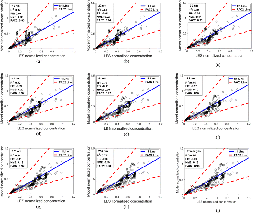
For clarity, Fig. 6 shows the ground-level concentrations for the 15 test cases predicted by the parametrized Gaussian-based model against that from our CTAG simulations for 8 particle sizes and the tracer gas, while Fig. S8† shows the concentration for the remaining particle size 180 nm. The concentrations were normalized by the no-barrier ground-level concentrations at each respective wind speed located at the roadside front of the vegetation barrier. The NME ranged between 0.18 and 0.3, the FB ranged between −0.12 and 0.09, and the FAC2 ranged between 0.93 and 0.98 across all particle sizes and the tracer gas, which is within an acceptable range. The R2 value ranged from 0.47 to 0.75. The lowest R2 of 0.47 was from the 15 nm particle size. This is likely due to the smallest size experiencing strong deposition compared to other particle sizes (30–253 nm) and since the parametrized Gaussian-based model is fitted for all particles, there might be a slight bias towards the size fraction with the majority number of particles. Overall, the parametrized Gaussian-based model showed favorable performance and was capable of capturing pollutant concentration behavior downwind of vegetative barriers. We also provide the concentrations versus downwind distance plots for particle sizes 15 and 253 nm at three different heights: ground level, breathing height, and mid-canopy for all test cases in Section S9 of the ESI.† Those plots demonstrate that there is reasonable agreement between the proposed Gaussian model and CTAG simulations and that the model can capture the downwind pollutant decay.
 |
| | Fig. 6 CTAG (LES) versus the parameterized Gaussian-based model using the multi-regime approach for normalized ground level concentrations for all 15 test cases evaluated at 30 locations within and downwind of the barrier. (a) 15 nm; (b) 22 nm; (c) 30 nm; (d) 43 nm; (e) 60 nm; (f) 88 nm; (g) 126 nm; (h) 253 nm; (i) tracer gas. | |
4.2 Vertical profile analysis
Fig. 7 shows the average R2, FB, and NME across all the vertical profiles within the vegetation to 15H downwind of the barrier, averaged across all 15 test cases for each particle size and the tracer gas. For most particle sizes and the tracer gas, the R2 value is ≥0.76, but the R2 value is lower for particles 15 and 22 nm. As discussed earlier, that could be due to the parametrized Gaussian-based model being biased towards the majority of particles (30–253 nm) which do not experience as much deposition as particles 15 and 22 nm. The FB was negative across all particle sizes and tracer gas, which indicates that the parameterized Gaussian-based model tended to slightly underestimate the vertical concentrations (Fig. 7b), however, it was within a satisfactory range. Finally, the NME ranged from 0.38 to 0.45 which is acceptable. We also performed the same analysis for each of the four regimes and we report the R2, FB, and NME for them in Section S10 of the ESI.† We also compared normalized vertical concentration profiles at three different locations for all test cases for particle sizes 15 and 253 nm and included them in Section S11 of the ESI.†
 |
| | Fig. 7 Evaluation metrics for the parameterized Gaussian-based model using the multi-regime approach averaged across all the vertical locations from within the vegetation to 15H downwind of the barrier. The average metrics are listed for all 9 particle sizes and the tracer gas (a) R2; (b) FB; (c) NME. | |
4.3 Sensitivity analysis: single row of vegetation and hedges/bushes
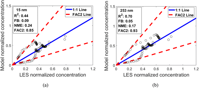
The parameterized Gaussian-based model was parameterized on cases that reflect barriers with two rows of vegetation. However, implemented vegetation barriers can consist of fewer or more rows. In areas where there is limited planting space, one row of vegetation could be the only viable option. To explore whether the parameterized Gaussian-based model is robust enough to capture the behavior of vegetation barriers with a single row of vegetation, we conducted a sensitivity analysis. We simulated four cases that represented vegetation with a single row to test the performance of the parameterized Gaussian-based model. The parameters of those cases are listed in Table S4 the ESI.†Fig. 8 shows the ground-level concentrations for the 4 single row test cases predicted by the parameterized Gaussian-based model versus that from our LES simulations for particle sizes of 15 and 253 nm. The results show that the parameterized Gaussian-based model predicted the concentrations for a single row of vegetation with R2 value 0.44–0.70 and an NME of 0.17–0.24, indicating favorable performance at predicting concentrations for single row vegetation barriers.
 |
| | Fig. 8 CTAG (LES) versus the parameterized Gaussian-based model normalized ground level concentrations for all 4 cases of vegetation with a single row of vegetation. (a) 15 nm; (b) 253 nm. | |
Since the simulated cases represent coniferous vegetation, it is important to understand whether the parameterized Gaussian-based model will be applicable to other types of vegetation. Studies have shown that hedges and bushes are effective roadside vegetation barriers and tend to have a uniform LAD profile with respect to height. We simulated 4 cases with uniform LAD profiles and compared the results to that of a coniferous LAD profile. The predicted concentrations were similar for both profiles with some discrepancies for deposition-dominated scenarios which is discussed in Section S13 of the ESI.† This highlights that the parameterized Gaussian-based model can provide useful predictions for vegetative barriers designed from hedges or bushes.
4.4 Limitations
There are many factors that could influence pollutant concentration that were not considered in this study which included wind direction, vehicle-induced turbulence, presence of buildings, and atmospheric stability. Capturing all those effects would require substantial simulations which is computationally expensive and could be an area of future study. Therefore, we focused on exploring the effects of a wide range of vegetation with varying dimensions and density. Furthermore, the performance of the parameterized Gaussian-based model was ideal within the parameter space explored in this study.
5. Conclusion
We developed a multi-regime approach that parameterized the Gaussian plume equations to characterize pollutant dispersion and deposition by roadside vegetation barriers. The parameterized Gaussian-based model accounted for the physical mechanisms of the barrier-related pollution dispersion. This occurred by identifying and capturing the behavior in four regimes: the vegetation, wake, transition, and recovery regimes. Deposition and dispersion were considered by describing the Gaussian plume equations parameters (mean plume velocity, vertical spread, emission rate, and source height) in each of the four regimes. To describe these parameters, a fit based on the vegetation properties and local wind speed was conducted. Seventy-five high-fidelity CFD simulations using the CTAG model, reflective of a wide range of vegetation barriers (heights 2–10 m, width: 2.5–13 m, LAI: 4–11) and wind speed (1–5 ms−1), were used to develop and evaluate the parameterized Gaussian-based model. The proposed model was therefore applicable to a wide range of vegetation barrier designs. The multi-regime parameterized Gaussian-based model's normalized mean error (NME) ranged between 0.18 and 0.3, the fractional bias (FB) ranged between −0.12 and 0.09, and R2 value ranged from 0.47 to 0.75 across all particle sizes and the tracer gas for ground level concentrations. The proposed model is the first to parameterize the Gaussian plume equations to describe the deposition and dispersion effects of vegetation barriers and can be used to help predict pollutant concentrations downwind of vegetation barriers.
Conflicts of interest
There are no conflicts to declare.
Acknowledgements
The Cornell team acknowledges support from the National Science Foundation (NSF) through grant no. 1605407. Mention of trade names or commercial products does not constitute endorsement or recommendation for use. The views expressed in this journal article are those of the authors and do not necessarily reflect the views or policies of the US Environmental Protection Agency.
References
-
HEI, Traffic-Related Air Pollution: A Critical Review of the Literature on Emissions, Exposure, and Health Effects, Health Effects Institute, Boston, MA, 2010, Report No.: HEI Special Report 17 Search PubMed.
- S. L. Kingsley, M. N. Eliot, L. Carlson, J. Finn, D. L. MacIntosh and H. H. Suh,
et al., Proximity of US schools to major roadways: a nationwide assessment, J. Exposure Sci. Environ. Epidemiol., 2014, 24(3), 253–259 CrossRef PubMed.
-
EPA, Near Roadway Air Pollution and Health: Frequently Asked Questions, Office of Transportation and Air Quality, United States Environmental Protection Agency, 2014 Search PubMed.
- D. Houston, M. Krudysz and A. Winer, Diesel Truck Traffic in Low-income and Minority Communities Adjacent to Ports Environmental Justice Implications of Near-Roadway Land Use Conflicts, Transp. Res. Rec., 2008,(2067), 38–46 CrossRef.
- M. L. Miranda, S. E. Edwards, M. H. Keating and C. J. Paul, Making the Environmental Justice Grade: The Relative Burden of Air Pollution Exposure in the United States, Int. J. Environ. Res. Public Health, 2011, 8(6), 1755–1771 CrossRef PubMed.
- J. Gallagher, R. Baldauf, C. H. Fuller, P. Kumar, L. W. Gill and A. McNabola, Passive methods for improving air quality in the built environment: a review of porous and solid barriers, Atmos. Environ., 2015, 120, 61–70 CrossRef CAS.
- R. Baldauf, Roadside vegetation design characteristics that can improve local, near-road air quality, Transp. Res. D: Transp. Environ., 2017, 52, 354–361 CrossRef PubMed.
- A. Tiwari, P. Kumar, R. Baldauf, K. M. Zhang, F. Pilla and S. Di Sabatino,
et al., Considerations for evaluating green infrastructure impacts in microscale and macroscale air pollution dispersion models, Sci. Total Environ., 2019, 672, 410–426 CrossRef CAS PubMed.
- K. V. Abhijith and P. Kumar, Field investigations for evaluating green infrastructure effects on air quality in open-road conditions, Atmos. Environ., 2019, 201, 132–147 CrossRef CAS.
- J. T. Steffens, Y. J. Wang and K. M. Zhang, Exploration of effects of a vegetation barrier on particle size distributions in a near-road environment, Atmos. Environ., 2012, 50(1), 120–128 CrossRef CAS.
- K. Hashad, B. Yang, R. W. Baldauf, P. Deshmukh, V. Isakov and K. M. Zhang, Enhancing the local air quality benefits of roadside green infrastructure using low-cost, impermeable, solid structures (LISS), Sci. Total Environ., 2020, 717, 137136 CrossRef CAS PubMed.
- P. Deshmukh, V. Isakov, A. Venkatram, B. Yang, K. M. Zhang and R. Logan,
et al., The effects of roadside vegetation characteristics on local, near-road air quality, Air Qual., Atmos. Health, 2019, 12(3), 259–270 CrossRef CAS PubMed.
- G. S. W. Hagler, M.-Y. Lin, A. Khlystov, R. W. Baldauf, V. Isakov and J. Faircloth,
et al., Field investigation of roadside vegetative and structural barrier impact on near-road ultrafine particle concentrations under a variety of wind conditions, Sci. Total Environ., 2012, 419, 7–15 CrossRef CAS PubMed.
- M. Y. Lin, G. Hagler, R. Baldauf, V. Isakov, H. Y. Lin and A. Khlystov, The effects of vegetation barriers on near-road ultrafine particle number and carbon monoxide concentrations, Sci. Total Environ., 2016, 553, 372–379 CrossRef CAS PubMed.
- Z. M. Tong, R. W. Baldauf, V. Isakov, P. Deshmukh and K. M. Zhang, Roadside vegetation barrier designs to mitigate near-road air pollution impacts, Sci. Total Environ., 2016, 541, 920–927 CrossRef CAS PubMed.
- J.-L. Santiago, R. Buccolieri, E. Rivas, H. Calvete-Sogo, B. Sanchez and A. Martilli,
et al., CFD modelling of vegetation barrier effects on the reduction of traffic-related pollutant concentration in an avenue of Pamplona, Spain, Sustain. Cities Soc., 2019, 48, 101559 CrossRef.
- K. Hashad, J. Gu, B. Yang, M. Rong, E. Chen and X. Ma,
et al., Designing roadside green infrastructure to mitigate traffic-related air pollution using machine learning, Sci. Total Environ., 2021, 773, 144760 CrossRef CAS PubMed.
- D. K. Heist, S. G. Perry and L. A. Brixey, A wind tunnel study of the effect of roadway configurations on the dispersion of traffic-related pollution, Atmos. Environ., 2009, 43(32), 5101–5111 CrossRef CAS.
- D. Finn, K. L. Clawson, R. G. Carter, J. D. Rich, R. M. Eckman and S. G. Perry,
et al., Tracer studies to characterize the effects of roadside noise barriers on near-road pollutant dispersion under varying atmospheric stability conditions, Atmos. Environ., 2010, 44(2), 204–214 CrossRef CAS.
- N. Schulte, M. Snyder, V. Isakov, D. Heist and A. Venkatram, Effects of solid barriers on dispersion of roadway emissions, Atmos. Environ., 2014, 97, 286–295 CrossRef CAS.
- A. Venkatram, V. Isakov, P. Des'hmukh and R. Baldauf, Modeling the impact of solid noise barriers on near road air quality, Atmos. Environ., 2016, 141, 462–469 CrossRef CAS.
- F. E. Ahangar, D. Heist, S. Perry and A. Venkatram, Reduction of air pollution levels downwind of a road with an upwind noise barrier, Atmos. Environ., 2017, 155, 1–10 CrossRef PubMed.
- B. Lalic and D. T. Mihailovic, An empirical relation describing leaf-area density inside the forest for environmental modeling, J. Appl. Meteorol., 2004, 43(4), 641–645 CrossRef.
- Y. J. Wang, A. DenBleyker, E. McDonald-Buller, D. Allen and K. M. Zhang, Modeling the chemical evolution of nitrogen oxides near roadways, Atmos. Environ., 2011, 45(1), 43–52 CrossRef CAS.
- Y. J. Wang and K. M. Zhang, Coupled turbulence and aerosol dynamics modeling of vehicle exhaust plumes using the CTAG model, Atmos. Environ., 2012, 59, 284–293 CrossRef CAS.
- Y. J. Wang, M. T. Nguyen, J. T. Steffens, Z. M. Tong, Y. G. Wang and P. K. Hopke,
et al., Modeling multi-scale aerosol dynamics and micro-environmental air quality near a large highway intersection using the CTAG model, Sci. Total Environ., 2013, 443, 375–386 CrossRef CAS PubMed.
- M. Germano, U. Piomelli, P. Moin and W. H. Cabot, A dynamic subgrid-scale eddy viscosity model, Phys. Fluids A, 1991, 3(7), 1760–1765 CrossRef.
- P. J. Richards, Appropriate boundary conditions for computational wind engineering models using the k–∈ turbulence model, J. Wind. Eng. Ind. Aerodyn., 1993, 46–47, 145–153 CrossRef.
- G. G. Katul, L. Mahrt, D. Poggi and C. Sanz, One- and two-equation models for canopy turbulence, Bound.-Layer Meteorol., 2004, 113(1), 81–109 CrossRef.
- T. Tahvanainen and E. Forss, Individual tree models for the crown biomass distribution of Scots pine, Norway spruce and birch in Finland, For. Ecol. Manage., 2008, 255(3–4), 455–467 CrossRef.
- N. R. Wilson and R. H. Shaw, A Higher Order Closure Model for Canopy Flow, J. Appl. Meteorol., 1977, 16(11), 1197–1205 CrossRef.
- R. H. Shaw and U. Schumann, Large-eddy simulation of turbulent flow above and within a forest, Bound.-Layer Meteorol., 1992, 61(1–2), 47–64 CrossRef.
- L. M. Zhang, S. L. Gong, J. Padro and L. Barrie, A size-segregated particle dry deposition scheme for an atmospheric aerosol module, Atmos. Environ., 2001, 35(3), 549–560 CrossRef CAS.
- Y. Pan, M. Chamecki and S. A. Isard, Large-eddy simulation of turbulence and particle dispersion inside the canopy roughness sublayer, J. Fluid Mech., 2014, 753, 499–534 CrossRef.
- C. W. Miller, An examination of Gaussian plume dispersion parameters for rough terrain, Atmos. Environ., 1978, 12(6–7), 1359–1364 CrossRef.
- M. G. Snyder, A. Venkatram, D. K. Heist, S. G. Perry, W. B. Petersen and V. Isakov, RLINE: a line source dispersion model for near-surface releases, Atmos. Environ., 2013, 77, 748–756 CrossRef CAS.
- A. Venkatram, M. G. Snyder, D. K. Heist, S. G. Perry, W. B. Petersen and V. Isakov, Re-formulation of plume spread for near-surface dispersion, Atmos. Environ., 2013, 77, 846–855 CrossRef CAS.
|
| This journal is © The Royal Society of Chemistry 2024 |
Click here to see how this site uses Cookies. View our privacy policy here.  Open Access Article
 *a
*a


![[thin space (1/6-em)]](https://www.rsc.org/images/entities/char_2009.gif) :
:![[thin space (1/6-em)]](https://www.rsc.org/images/entities/char_2009.gif) 3, which represents coniferous vegetation, and was used in previous studies.29,30 The vegetation barrier consisted of two rows of vegetation to ensure that it had no gaps in it; therefore, the barrier's width to height ratio was 4
3, which represents coniferous vegetation, and was used in previous studies.29,30 The vegetation barrier consisted of two rows of vegetation to ensure that it had no gaps in it; therefore, the barrier's width to height ratio was 4![[thin space (1/6-em)]](https://www.rsc.org/images/entities/char_2009.gif) :
:![[thin space (1/6-em)]](https://www.rsc.org/images/entities/char_2009.gif) 3. In addition, we explored three LAI values 4, 7, and 11 to reflect various vegetation density values which account for a wide range of vegetation (Asner et al., 2003). Different urban conditions were considered by covering a range of velocities from 1 to 5 ms−1 at a height of 10 m. In total, we simulated 75 cases which highlighted 5 different barrier heights, 5 different velocities, and three different LAI values as shown in Table 1. The 75 CTAG-generated cases were randomly split into 60 cases to train the parameterized Gaussian-based model, and 15 cases to test it representing an 80/20% split. The test cases were not used in any training to ensure rigorous evaluations. In addition to the 75 cases, we simulated 5 other cases with no barrier at five different wind speeds to normalize the results and understand the impact of the barrier compared to no vegetation.
3. In addition, we explored three LAI values 4, 7, and 11 to reflect various vegetation density values which account for a wide range of vegetation (Asner et al., 2003). Different urban conditions were considered by covering a range of velocities from 1 to 5 ms−1 at a height of 10 m. In total, we simulated 75 cases which highlighted 5 different barrier heights, 5 different velocities, and three different LAI values as shown in Table 1. The 75 CTAG-generated cases were randomly split into 60 cases to train the parameterized Gaussian-based model, and 15 cases to test it representing an 80/20% split. The test cases were not used in any training to ensure rigorous evaluations. In addition to the 75 cases, we simulated 5 other cases with no barrier at five different wind speeds to normalize the results and understand the impact of the barrier compared to no vegetation.
![[D with combining tilde]](https://www.rsc.org/images/entities/i_char_0044_0303.gif) p)LAD(z)
p)LAD(z)![[D with combining tilde]](https://www.rsc.org/images/entities/i_char_0044_0303.gif) p) is the average particle concentration of a particle size Dp, and Vd(Dp) is the deposition velocity adopted from a widely used dry deposition model.33 To assess if the proposed multi-regime parametrized Gaussian-based model captured the deposition and dispersion of the vegetation barrier, the performance for each of the 9 particle sizes and the tracer gas is provided. The governing equations for momentum, dispersion, and deposition are included in Section S2 of the ESI.† The CTAG model highlighted in this section aligns with those used in our previous studies.10,11,15
p) is the average particle concentration of a particle size Dp, and Vd(Dp) is the deposition velocity adopted from a widely used dry deposition model.33 To assess if the proposed multi-regime parametrized Gaussian-based model captured the deposition and dispersion of the vegetation barrier, the performance for each of the 9 particle sizes and the tracer gas is provided. The governing equations for momentum, dispersion, and deposition are included in Section S2 of the ESI.† The CTAG model highlighted in this section aligns with those used in our previous studies.10,11,15


![[thin space (1/6-em)]](https://www.rsc.org/images/entities/char_2009.gif) C1 = 0.022Lm−1.231 − 0.0149
C1 = 0.022Lm−1.231 − 0.0149![[thin space (1/6-em)]](https://www.rsc.org/images/entities/char_2009.gif) C2 = (0.089Lm + 0.8) (−0.002U10)
C2 = (0.089Lm + 0.8) (−0.002U10)![[thin space (1/6-em)]](https://www.rsc.org/images/entities/char_2009.gif) C3 = (0.003LAI − 0.008) (0.44U10 − 0.33)
C3 = (0.003LAI − 0.008) (0.44U10 − 0.33)![[thin space (1/6-em)]](https://www.rsc.org/images/entities/char_2009.gif) C4 = (−0.44Lm−1.82 + 1.19) (0.054U10 − 0.016),
C4 = (−0.44Lm−1.82 + 1.19) (0.054U10 − 0.016),![[thin space (1/6-em)]](https://www.rsc.org/images/entities/char_2009.gif) B1 = 0.037H−1.505 + 0.07
B1 = 0.037H−1.505 + 0.07![[thin space (1/6-em)]](https://www.rsc.org/images/entities/char_2009.gif) B2 = 0.013
B2 = 0.013![[thin space (1/6-em)]](https://www.rsc.org/images/entities/char_2009.gif) B3 = (6.95 × 10⁻⁴)H × LAI
B3 = (6.95 × 10⁻⁴)H × LAI![[thin space (1/6-em)]](https://www.rsc.org/images/entities/char_2009.gif) B4 = (6.95 × 10⁻⁴)H × LAI
B4 = (6.95 × 10⁻⁴)H × LAI