Using a supervised machine learning approach to predict water quality at the Gaza wastewater treatment plant

Abstract

This paper presents the use of four machine learning algorithms including Gaussian process regression (GPR), random forest (FR), extreme gradient boosting (XGB) and light gradient boosting machine (LightGBM) to predict the concentration of total suspended solids (TSS), chemical oxygen demand (COD), and biochemical oxygen demand (BOD) in the effluent of the Gaza wastewater treatment plant one day ahead. Data was collected from 360 wastewater samples taken from the Gaza wastewater treatment plant, and five input parameters were used in the proposed method: pH_inf, temperature (Temp_inf), BOD_inf, TSS_inf, and COD_inf. Four error measures were used to evaluate the prediction accuracy of the models. Results showed that the GPR model in the testing datasets is the best predictive model for predicting the effluent's TSS, COD and BOD with the best accuracy in relation to the correlation coefficient (CC), that is, (0.964–0.950–0.975) against RF (0.932–0.910–0.943), XGB (0.916–0.901–0.954), and LightGBM (0.890–0.892–0.883). The importance of input parameters was assessed, and temperature and pH were found to be the most important parameters in wastewater quality predictions using these four models. The study concluded that GPR is the most representative model. The model may help users in selecting optimal wastewater treatment based on original characteristics and standards.

---

Environmental significance

The article “Using a supervised machine learning approach to predict water quality at the Gaza wastewater treatment plant” holds substantial environmental significance. By employing supervised machine learning algorithms, the research aims to predict water quality parameters at the Gaza wastewater treatment plant. Accurate prediction of water quality is essential for effective monitoring and management, ensuring the protection of public health and the environment. By leveraging machine learning algorithms, the study seeks to enhance the understanding and predictive capabilities of water quality assessment, enabling proactive interventions and timely decision-making. The findings can contribute to optimizing wastewater treatment processes, reducing the discharge of pollutants, and improving the overall efficiency of the treatment plant. Ultimately, the research holds promise for enhancing water resource sustainability, safeguarding ecosystem health, and promoting the well-being of communities relying on the wastewater treatment plant in Gaza.

1 Introduction

Freshwater is crucial for various aspects of human life, including economic development, environmental sustainability, and the reduction of poverty and sickness.^1,2 However, due to industrial contamination, population growth, and wastewater from agricultural activities, the scarcity of freshwater sources has become a significant problem.³ Wastewater treatment is a crucial technology that could provide new sources of water while also reducing the burden on the environment by removing organic pollutants.⁴ Due to the nonlinear and dynamic nature of the process, monitoring the effluent water quality is essential to ensure proper operation of wastewater treatment plants.⁵ However, traditional monitoring methods are labor-intensive, expensive, and unable to be used online. Management measures are needed to ensure that effluent quality indicators are functioning properly. While some effluent water indicators can now be measured online using wireless sensor networks, measuring parameters such as biochemical oxygen demand (BOD) and chemical oxygen demand (COD) remains challenging due to high costs and sensor constraints.⁶ Since high levels of BOD can result in water eutrophication, which can impact human health, controlling BOD effluent concentrations is critical. Machine learning techniques are used to train models that can detect abnormal operational circumstances in wastewater treatment plants (WWTPs).⁷ Machine learning models can be highly useful in wastewater treatment processes due to their complexity and multivariable control, nonlinearity, and parameter dependencies that fluctuate over time. Utilizing temporal information can lead to better predictions. Although only a few studies have used neural networks like RNNs for modeling WWTP processes,⁸ artificial intelligence, a subset of machine learning techniques, focuses on identifying patterns in data and drawing conclusions for forecasting future data. Techniques such as artificial neural networks (ANN), support vector machine (SVM) decision trees (DT), random forests (RF), and ensemble learning have broad applications in fields like text processing, computer vision, healthcare, finance, and robotics, as well as socioeconomic and environmental research.^9–12 Capodaglio et al. (1991)¹³ used artificial neural networks and stochastic models to predict bulking conditions that lead to inferior effluent quality in activated sludge. Qiao et al. (2019)¹⁴ developed a recurrent fuzzy neural network (RFNN) based strategy to regulate concentrations in a WWTP. Dairi et al. (2019)¹⁵ used unsupervised and deep learning to develop an anomaly detection model to catch any faults that arise during operation. Mamandipoor et al. (2020)¹⁶ focused on fault identification in a WWTP, while Wang et al. (2019)¹⁷ demonstrated the real-time predictability of COD using convolutional neural network-long short-term memory (CNN-LSTM) models. Pisa et al. (2018)¹⁸ developed forecasting models employing gated recurrent neural networks to forecast the amount of intake to the plant. de Canete et al. (2016)¹⁹ examined the use of gray model and ANN techniques to forecast suspended matter and chemical oxygen demand in the wastewater treatment process. A mixed soft sensor model based on a wavelet neural network and adaptive weighted fusion was developed by Cong & Yu,²⁰ for online prediction of effluent COD. The performance of a wastewater treatment plant was evaluated using ANN and a multiple linear regression approach by Hamada et al. (2018).²¹ Zeinolabedini and Najafzadeh (2019)²² demonstrated that adding different parent wavelet functions to the neural network structure increased the precision of estimating the volume of wastewater sludge. Kadam et al. (2019)²³ employed ANN and multiple linear regression to model and predict water quality characteristics in river basins, while Heddam et al. (2016)²⁴ studied a generalized regression neural network model to estimate the BOD of effluent in wastewater treatment plants. Nourani et al. (2018)²⁵ demonstrated the reliability of a neural network ensemble's prediction ability. SVM is a prediction technique that can build high-dimensional data models with small sample sizes and has good generalizability compared to the ANN method.²⁶ SVM-based prediction has been extensively researched for tracking and forecasting intake conditions and sludge volume index in wastewater treatment plants.²⁷ An adaptive multi-output soft sensor model,²⁸ hybrid linear–nonlinear method,²⁹ data-based predictive control technique,³⁰ and SVM model^31,32 have also been used to predict effluent index, total solid content, and water quality of wastewater treatment facilities. The least-squares support vector machine (LSSVM) has been presented as a solution to the drawbacks of SVM for large datasets.³³ Swarm intelligence optimization algorithms have been combined with machine learning techniques, such as particle swarm optimization (PSO) and support vector machines,³⁴ self-organizing radial basis function neural networks,³⁰ and artificial bee colony optimization back-propagation networks,³⁵ to increase accuracy and reduce processing time. Prediction interval is a common method to calculate prediction uncertainty, which has been integrated with a recurrent neural network using a mean variance estimation method.³⁶

In light of the numerous challenges associated with recording and measuring wastewater quality, particularly in the case of parameters such as BOD and COD, our study's primary objective is to assess the effectiveness of four different machine learning algorithms: GPR, RF, XGB, and LightGBM. Our aim is to predict the concentrations of post-treated variables, specifically TSS_eff, COD_eff, and BOD_eff, within the Gaza wastewater treatment plant and present an exceptional perspective on addressing these issues. What truly distinguishes our research is the careful collection of data from an extensive dataset counting 360 wastewater samples, all thoroughly sourced from a wastewater treatment plant within Gaza. These samples serve as the grounding for our predictive models, supported by a thoughtful selection of five essential input parameters, including pH_inf, temperature (Temp_inf), BOD_inf, TSS_inf, and COD_inf. Our study presents a comprehensive examination, employing these five input parameters to identify the most accurate predictive model for each effluent parameter. Additionally, we carry out the assessment of variable importance among these input parameters, shedding light on the factors that significantly influence wastewater quality predictions. Furthermore, our study endeavors to pinpoint the most representative models tailored to the dataset at hand. This multifaceted approach not only accelerates computation time for assessing wastewater treatment plants but also harnesses various physicochemical characteristics as input parameters for predicting treatment indicators. By extending our predictive capabilities to effluent wastewater quality parameters, our study offers invaluable insights for stakeholders across various sectors. It prepares them with the means to make well-informed decisions pertaining to wastewater treatment, enabling them to measure compliance with legal requirements concerning wastewater disposal and reuse. Moreover, it provides a good understanding of the potential consequences of discharging treated wastewater into Gaza's coastal environment. These predictive models hold utility for a diverse spectrum of stakeholders, including farmers, producers, processors, technology providers, consultants, and regulators, all vested in assessing and mitigating wastewater contamination levels. In essence, our research represents a significant step forward in addressing the complex challenges surrounding wastewater quality management.

2 Materials and methods

2.1 Description of the study area

The Gaza Strip is a small region located on the southern edge of the Palestinian coastal plains, with a 42 km coastline on the Mediterranean Sea.³⁷ With a population of 2.1 million and a growth rate of 2.8 percent by the end of 2021, the Gaza Strip had a high population density when compared to other regions of the world (5936 people per km²).³⁸ All of the rainfall in the arid to semi-arid region where the Gaza Strip is located occurs between October and April. The average seasonal precipitation varies significantly by area, with 474 mm per year in the north and 250 mm per year in the south.³⁹ The study area for this study is the Gaza wastewater treatment plant, also known as the Sheikh Eglin Plant, located southwest of Gaza City. The plant has five anaerobic basins and treated wastewater is discharged into the Mediterranean, while sludge production is disposed of in landfills on the eastern side of Gaza City. There are occasional leaks of sludge and wastewater into surrounding rural areas. Sewage and sludge disposal have been a continuous process in the Gaza Strip since 1977. Each day, around 80 000 cubic meters of wastewater are received, while the plant has a capacity of only 60 000 cubic meters. The remaining 20 000 cubic meters of untreated sewage are transported to the central plant situated in Al-Bureij, to the east of Gaza City. The GWWTP plant has two divisions: the operation section and the laboratory, responsible for daily plant activities and quality control, respectively. The semi-secondary treatment process consists of anaerobic lagoons, trickling filters, sedimentation tanks, and a pumping station before discharging treated wastewater into the Mediterranean Sea. The sludge produced, at a rate of 20 tons per day, is stored in anaerobic ponds and transferred to central solid waste disposal due to a lack of sludge treatment facilities.

2.2 Data collection and preprocessing

In order to conduct this study, data on the inlet and outlet wastewater quality were collected from the Palestinian Water Authority and Gaza Municipality for one year in 2020. After collecting the datasets, efforts were made to appropriately understand the required data. Upon examination of the data, it was found that some readings had significant variations due to a lack of treatment process in the wastewater treatment plant and occasional station malfunctions. The study aims to investigate the potential for creating a machine learning model to predict wastewater quality parameters such as BOD_eff, COD_eff, and TSS_eff. All data collected for this study covered a comprehensive dataset of 360 measurements, which included exactly resolved missing values. It's worth noting that these measurements were attained as rapid samples taken on a given day. Significantly, the majority of these measurements were largely unaffected by rain runoff, primarily due to the stringent filtration processes employed in the treatment system. This careful data collection approach and the effectiveness of the filtration system together ensured the reliability and integrity of the dataset, allowing for a more accurate and meaningful analysis of the water quality parameters under investigation. All data gathered were pooled into one set for analysis. The primary measurable indicators for wastewater quality were temperature, pH, BOD, COD, and TSS. Rescaling the data is recommended as input and output variables have vastly different orders of magnitude, leading to more accurate predictions. While “0, 1” is typically used for data normalization, the variables in this study are rescaled to fall within the range of 0 to 1 to accommodate all data sets used to create ML prediction models.⁴⁰ The selection of machine learning model input and output variables that will have a substantial impact on the prediction of effluent BOD, COD, and TSS requires engineering judgment. A branded constructive algorithm is deployed to the network after adequate training and testing using the Python software. To smooth the data and remove outliers, a boxplot filter is applied to the collected data in this study.⁴¹ Therefore, model hyperparameters were set for all models during model calibration. Table 1 shows the descriptive statistics of the observed WWTP variables, including the maximum, minimum, mean, standard deviation, variance, and skewness, which are represented by the letters Xmax, Xmin, mean, SD, Cv, and skew, respectively.

Table 1 Basic statistics of Gaza WWTP water quality

Parameters	Min	Mean	SD	Max	Cv	Skewness	WHO standards
T influent (°C)	13.8	22.66	4.26	32	18.19	0.1863	—
pHinfluent	6.75	7.81	0.22	8.56	0.0493	−0.4097	—
TSSinfluent (mg L^−1)	363	502.09	82.94	800	6880.59	0.9739	—
BODinfluent (mg L^−1)	380	497.51	73.86	840	5455.643	1.19157	—
CODinfluent (mg L^−1)	720	992.13	156.51	1520	24 496.8	0.80963	—
T effluent (°C)	14	22.60	4.24	31	17.98	0.1854	≤37 °C
pHeffluent	7.06	7.92	0.22	8.31	0.0493	−0.4073	6.5–8.5
TSSeffluent (mg L^−1)	42	113.21	40.24	300	1618.94	1.137	≤30 mg L^−1
BODeffluent (mg L^−1)	40	102.88	34.76	230	1208.57	0.5603	≤30 mg L^−1
CODeffluent (mg L^−1)	53	228.42	75.73	412	5735.49	0.2755	≤125 mg L^−1

---

2.3 Proposed machine learning models

In supervised learning, a set of input observations with their corresponding known output values are used to train machine learning algorithms to create universal rules or “models” that can predict the outcome of new and unseen data. There are two main types of supervised learning: classification, which deals with categorical results, and regression, which deals with numerical results.⁴² In our study, we employed Python software as our primary tool to train and implement four different machine learning algorithms, namely GPR, RF, extreme gradient boosting (XGBoost), and LightGBM. These algorithms were harnessed to predict wastewater indicators within the context of the Gaza wastewater treatment plant. Python served as the foundational platform for developing, optimizing, and evaluating these models, enabling us to deliver accurate and efficient predictions for wastewater management purposes.

2.3.1 RF. Random forest is a popular supervised machine learning method in water resource applications that combines classification and regression trees, with bagging and randomization techniques to generate more accurate predictions. Bagging involves creating a bootstrap sample from the real dataset and training the model ntree times using that sample. The prediction from bagging serves as the mean forecast made by ntree trained models. Randomization selects variables responsible for data partitioning at random to reduce the correlation between trees and decrease variation in predictions. RF is particularly user-friendly because it can process high-dimensional data without feature selection, is immune to noise, and has fast training speeds.²⁸ In Python, the scikit-learn library offers a comprehensive implementation of the RF model, rendering the training process accessible and straightforward. In our study, we sought to harness the full potential of the RF model by employing model tuning techniques. Specifically, we focused on altering two key hyperparameters during the training process:

• ntree (number of trees): we experimented with different values for the number of trees in the ensemble. After careful evaluation, it was determined that setting ntree = 300 resulted in the most favorable outcomes.

• mtry (number of variables for splitting): we also varied the number of variables considered for splitting at each tree node. Our findings indicated that setting mtry = 13 yielded the best results, characterized by the smallest out-of-bag error.

By fine-tuning these parameters, we aimed to enhance the predictive performance of our RF model, aligning it with the specific requirements of wastewater indicator prediction.^43,44

2.3.2 XGBoost. XGBoost is a popular technique in data mining projects¹¹ due to its ability to create many shallow decision trees that produce high accuracy predictions when combined. Regularization is used in XGBoost to prevent overfitting by minimizing an objective function and taking care of the loss function.⁴⁵ The model's hyperparameters, such as Eta, gamma, max depth, min child weight, nrounds, colsample bytree, and subsample, can be adjusted to optimize the XGBoost model.⁴⁶ In this study, we employed the XGBoost model for wastewater indicator prediction, a powerful and widely adopted gradient boosting algorithm. To optimize the performance of the XGBoost model, a thorough process of hyperparameter fine-tuning was conducted. The objective was to determine the ideal combination of hyperparameter values that would yield the most accurate predictions. After extensive experimentation and evaluation, the following hyperparameter values were selected based on their ability to minimize the root mean square error across all experimental groupings:

• Eta (learning rate): 0.07

• Gamma (minimum loss reduction to make a further partition on the leaf node): 0.5

• Max depth of trees: 4

• Min child weight (minimum sum of instance weight hessian to make a partition): 500

• Number of rounds (boosting iterations): 0.7

• Colsample bytree (fraction of features used in each boosting round): 0.7

• Subsample (fraction of data used in each boosting round): 0.7

These specific hyperparameter values were chosen as they consistently produced the lowest root mean square error values across all experimental groups. This thorough fine-tuning process ensured that the XGBoost model was optimized to deliver the highest predictive accuracy for wastewater indicator forecasting in the context of the Gaza wastewater treatment plant. It exemplifies the rigorous approach we undertook to enhance the model's performance and its utility in the present applications.

2.3.3 Gaussian process regression (GPR). Gaussian process regression is a supervised learning technique that is commonly used to solve regression and probabilistic classification problems. The name “Gaussian process” is derived from the fact that each Gaussian process is essentially an infinite-dimensional extension of multivariate Gaussian distributions.⁴⁷ In this article, the focus is on Gaussian processes used for regression purposes, which is known as Gaussian process regression. GPR has been applied to solve a diverse range of real-world problems, spanning various fields such as materials science, chemistry, engineering, environmental sciences, physics, and biology. In our specific study, we harnessed the power of GPR to tackle the task of optimizing the prediction performance for the variable ‘k.’ To accomplish this, we employed a systematic approach known as GridSearchCV, which is used for hyperparameter tuning. This technique enabled us to fine-tune the hyperparameters of the Gaussian process regression model, ultimately seeking to achieve the highest prediction accuracy for ‘k.’ Through our analysis, we identified that the optimal values for the basis function constant and the exponential kernel function were achieved when exploring a range of values for ‘k’, specifically set within the range of 1 to 10. This careful parameter tuning process allowed us to extract the most meaningful information from our data and enhance the predictive capabilities of the GPR model, resulting in more accurate and reliable predictions. The utilization of GridSearchCV showcased our commitment to rigorously optimizing the GPR model to suit the specific requirements of our study, ultimately yielding robust and meaningful insights.

2.3.4 LightGBM. The gradient boosting decision tree (GBDT) is an ensemble ML technique that utilizes multiple decision trees as base learners. GBDT is based on the classification and regression tree (CART) function and is implemented through LightGBM, which is an effective framework. GBDT is proposed with a graph-based algorithm, a gradient-based one-sided sampling algorithm, and an exclusive feature aggregation algorithm. These algorithms speed up the model training without compromising prediction accuracy or increasing memory loss.⁴⁸ However, GBDT's iteration process can result in slow training speed and large memory consumption. The chosen evaluation metrics for assessing the model's performance were set to include ‘l1’ and ‘l2’, enabling a comprehensive assessment of model accuracy and robustness. Additionally, several hyperparameters were thoughtfully configured to achieve the best results: learning rate: 0.005, feature fraction: 0.9, bagging fraction: 0.7, bagging frequency: 10, verbose: 0, max depth: 8, num leaves: 128, max bin: 512, and num iterations: 100 000. These accurately chosen hyperparameters and configurations collectively contributed to the model's ability to perform reasonably in predicting wastewater indicators. Their selection was driven by a keen understanding of the dataset and the nuances of the problem at hand. This comprehensive approach showcases our devotion to achieving the highest predictive accuracy and reliability using LightGBM.

2.4 Dataset quality and size effects on ML model performance

The quality and size of the dataset have a significant impact on the created model's superiority. Data must contain an adequate number of samples and must accurately reflect the complete range of all potential situations. For instance, in processes that are tied to the environment, the source dataset should comprise at least a full year's worth of measured data to guarantee that all seasonal influences are accounted for in the data. Large and representative subsets of data are needed for both training and validation in order for a model to be developed efficiently. Based on the platform of Python 3.9.7, the influent temperature, influent pH, influent TSS, influent COD and influent BOD were taken as an array to train the ML models. One year's worth of data from 2020 was utilized for both the training and testing stages. In this study, four machine learning algorithms were used including LightGBM, XGB, GPR, and RF to predict the effluent TSS_eff, effluent COD_eff and effluent BOD_eff concentrations of the Gaza wastewater treatment plant (Sheikh Ejleen WWTP). Before the suggested ML approaches were finalized, all the models underwent preliminary training to develop their ideal architectures. In this study, the split ratios of 80 : 20, 70 : 30, and 75 : 25 are initially used with the current dataset, with the dataset division being determined based on the minimal RMSE value reached through trial and error. The majority of the models got the lowest prediction errors during the training procedure with a dataset partition of 70 : 30. 252 readings, or 70% of the whole dataset, and 108 readings, or 30% of it, are used for training (calibration) and testing (validation), respectively, based on the findings. However, K-fold cross validation (CV), which has become widely used in multiple modeling linked to water resource studies, is used to verify the model hyper-parameter optimization.^49,50 However, in the current study, the model generalization error is assessed using K-fold cross-validation with a K value of 5 (i.e., k = 5) in order to enhance the performance of the suggested models.

2.5 Model performance evaluation

The accuracy of the model during training and testing is evaluated in this study using the root means square error (RMSE), mean absolute error (MAE), mean absolute percentage error (MAPE), and correlation coefficient (CC). A low MAPE number indicates high model fidelity, and vice versa.⁴² The mathematical formulations for the numerous metrics used are as follows.where X_k = observed value and Y_k = predicted value.where n is the number of error values; X_k is the actual observation time series values and Y_k is the predicted time series values.where X_k = actual observation time series values, Y_k = predicted time series values and N = is the number of error values

3 Results and discussion

3.1 WWTP data and correlation matrix analysis

Wastewater quality data was collected and utilised to train multiple machine learning (ML) algorithms for predicting BOD, COD, and TSS in wastewater effluents from the Gaza wastewater treatment plant. The data was entered into Microsoft Excel sheets, uploaded to Python version 3.9.7 software, and analysed using statistical tools such as minimum (min), maximum (max), mean, standard deviation, coefficient of variation, and skewness. Additionally, the correlation coefficient was used to measure the linear association among the wastewater quality parameters. Table 1 summarises the statistical analysis of the wastewater quality parameters used for training, and testing the prediction models.

Table 1 shows that water temperature varied by season, with influent ranging from 13.8 to 32 °C (mean 22.66 °C) and effluent ranging from 14 to 31 °C (mean 22.60 °C). Bacterial activity was promoted by a drop in temperature. Influent pH (6.75–8.56, mean 7.81) met WHO standards, while effluent pH (7.06–8.31, mean 7.92) decreased indicating treatment. Influent BOD (380–840 mg L⁻¹, mean 497.51 mg L⁻¹) was high due to organic materials, while effluent BOD (40–230 mg L⁻¹, mean 102.88 mg L⁻¹) showed successful biodegradation. Effluent COD (53–412 mg L⁻¹, mean 228.42 mg L⁻¹) and TSS (42–300 mg L⁻¹, mean 113.21 mg L⁻¹) were lower than influent due to treatment, though interference-causing substances may have affected COD. Insufficient sludge settlement caused high effluent TSS. Overall, the treatment plant was able to remove approximately 79.32% BOD, 77% COD, and 77.45% TSS, which decreased compared to historical data from previous years. This decline was due to miscalculations in design criteria, increased load, and maintenance issues. Currently, removal efficiencies range from 80–85% for BOD, COD, and TSS.

The treatment process in the Gaza wastewater treatment plant showed acceptable performance when it is compared with the wastewater treatment plant in Sidi Bel Abbes city in northwestern Algeria. The station operated with removal efficiencies higher than 91% for biological oxygen demand (BOD), chemical oxygen demand (COD) and total suspended solids (TSS) and produced high quality effluent.⁵¹ The study of correlation coefficient mostly measures the association between two or more functionally independent variables. The values of correlation coefficient during this study are calculated using Python 3.9.7 software (Table 2). Pearson's correlation was used to detect linear associations between various variables. Effluent BOD is inversely correlated with influent T, pH, BOD, and TSS and positively correlated with effluent COD and TSS. Effluent COD is inversely correlated with influent T, pH, BOD, TSS and positively correlated with effluent BOD and TSS. Effluent TSS is positively correlated with effluent BOD, COD and influent TSS and inversely correlated with influent T, pH, BOD and COD. Effluent BOD is found to be strongly correlated with effluent COD and TSS (r = 0.95 and 0.77) and moderately to weakly correlated with influent T, pH, BOD, COD and TSS. Effluent COD is correlated moderately to weakly with influent T, BOD, COD, and pH and poorly with influent TSS and correlated strongly with effluent BOD and TSS (r = 0.95 and 0.72). Effluent TSS is found to be strongly correlated with effluent BOD and COD (r = 0.77 and 0.72) and is correlated moderately to weakly with influent T and poorly with influent pH, BOD, COD and TSS.

Table 2 Correlation matrix of the study area dataset

	Temp.	pH	TSSinf	CODinf	BODinf	TSSeff	CODeff	BODeff
Temp.	1.000
pH	0.345	1.000
TSS	−0.012	0.13	1.000
COD	−0.059	0.045	0.8	1.000
BOD	0.077	0.15	0.69	0.84	1.000
TSSeff	−0.32	−0.048	0.023	−0.052	−0.18	1.000
CODeff	−0.44	−0.45	−0.0065	0.062	−0.19	0.72	1.000
BODeff	−0.48	−0.45	−0.017	0.014	−0.22	0.77	0.95	1.000

---

3.2 Machine learning prediction results

In this study, four different machine learning algorithms were employed to predict the effluent quality of the Gaza wastewater treatment plant, specifically the BOD, COD, and TSS indicators. The performance of the machine learning predictions is subsequently evaluated in the following sections.

3.2.1 Effluent TSS prediction. Table 3 presents the results obtained in terms of RMSE, MAE, CC, and MAPE values with the training and testing datasets for the prediction of TSS_eff concentration. Comparison of these values indicates a slight improvement in wastewater treatment plant performance with the adjusted GRP [RMSE = (7.61–18.28 mg L⁻¹), MAE = (6.83–7.65), CC = (0.985–0.964) and MAPE = (4.51–5.07%)] as compared to the RF [RMSE = (10.24–20.82 mg L⁻¹), MAE = (7.61–10.14), CC = (0.974–0.932) and MAPE = (5.02–6.70%)], XGB [RSME = (13.51–24.58), MAE = (8.86–12.82), CC = (0.977–0.916), and MAPE = (5.84–8.49%)], and MAPE = (6.30–11.10%)] and LightGBM [RMSE = (17.72–32.66 mg L⁻¹), MAE = (10.57–17.77), CC = (0.955–0.890) and MAPE = (6.97–11.77%).

Table 3 Predictive index of TSS_eff

Model	RMSE (mg L^−1)	MAE	CC	MAPE (%)
RF
Training dataset	10.29	7.61	0.979	5.02
Testing dataset	20.82	10.19	0.932	6.70
GPR
Training dataset	7.61	6.83	0.985	4.51
Testing dataset	18.28	7.65	0.964	5.07
XGB
Training dataset	13.51	8.86	0.977	5.84
Testing dataset	24.58	12.82	0.916	8.49
LightGBM
Training dataset	17.72	10.57	0.955	6.97
Testing dataset	32.66	17.77	0.890	11.77

---

Based on the results obtained, it is evident that the GPR model outperforms other regression models in terms of efficiency. However, the RF and XGB models also show good performance in predicting the effluent TSS concentration, while the LightGBM model has slightly lower performance when compared to the aforementioned models (as shown in Table 3). In this study, supervised learning-based algorithms, namely GPR, FR, XGB, and LightGBM, were trained and tested, and their performances were compared to determine the best prediction model. As presented in Table 3, the GPR model showed the highest accuracy during model training with an RMSE of 7.61 mg L⁻¹, MAE of 6.83, R of 0.985, and MAPE of 4.51% compared to other models, indicating that the GPR algorithm performs well with the current dataset. Additionally, during model testing, the GPR-based prediction model demonstrated the highest accuracy compared to the other three ML models with an RMSE of 18.28 mg L⁻¹, MAE of 7.65, R of 0.964, and MAPE of 5.07% (Table 3).

To better understand the accuracy of the developed models, a scatter plot is made from the fit line of the best-obtained model (Fig. 1). Fig. 1 shows the distribution of the effluent TSS predicted values of the developed models with respect to the test values, which are closer to the best-fit line in the case of the GPR model than the others, confirming the validity of the developed GPR model. From the figure it can be seen that the performance of GPR is slightly better than those of RF and XGB where these two models showed better performance than LightGBM. In general, the GPR model agreed well with the actual values in the testing phase, while this was not the case for the LightGBM model. The LightGBM model obtained the weakest performance in the training and testing phases. Based on the obtained CC values, the performance of the predictive models in the present study followed the order of GPR > RF > XGB > LightGBM. In comparison to the study conducted by Hamada et al. (2018)²¹ where they utilized an MLP neural network model to predict the average monthly wastewater quality in the GWWT plant, our study took a different approach. Hamada's model had an RMSE of 37.38 mg L⁻¹, an R-value of 0.765, and an MAPE of 26.33% for TSS predictions during testing. In contrast, our study focused on predicting wastewater quality indicators one day ahead and employed a variety of methods. Remarkably, our findings revealed that the models we developed outperformed Hamada et al.'s MLP model when applied to the same study area. This suggests that our approach achieved superior accuracy in predicting wastewater quality, particularly in the context of TSS concentration. Furthermore, when comparing our study with other previous studies^52,53 it becomes evident that our predictive models consistently demonstrated good and satisfactory performance levels, supporting their effectiveness in enhancing wastewater quality prediction.

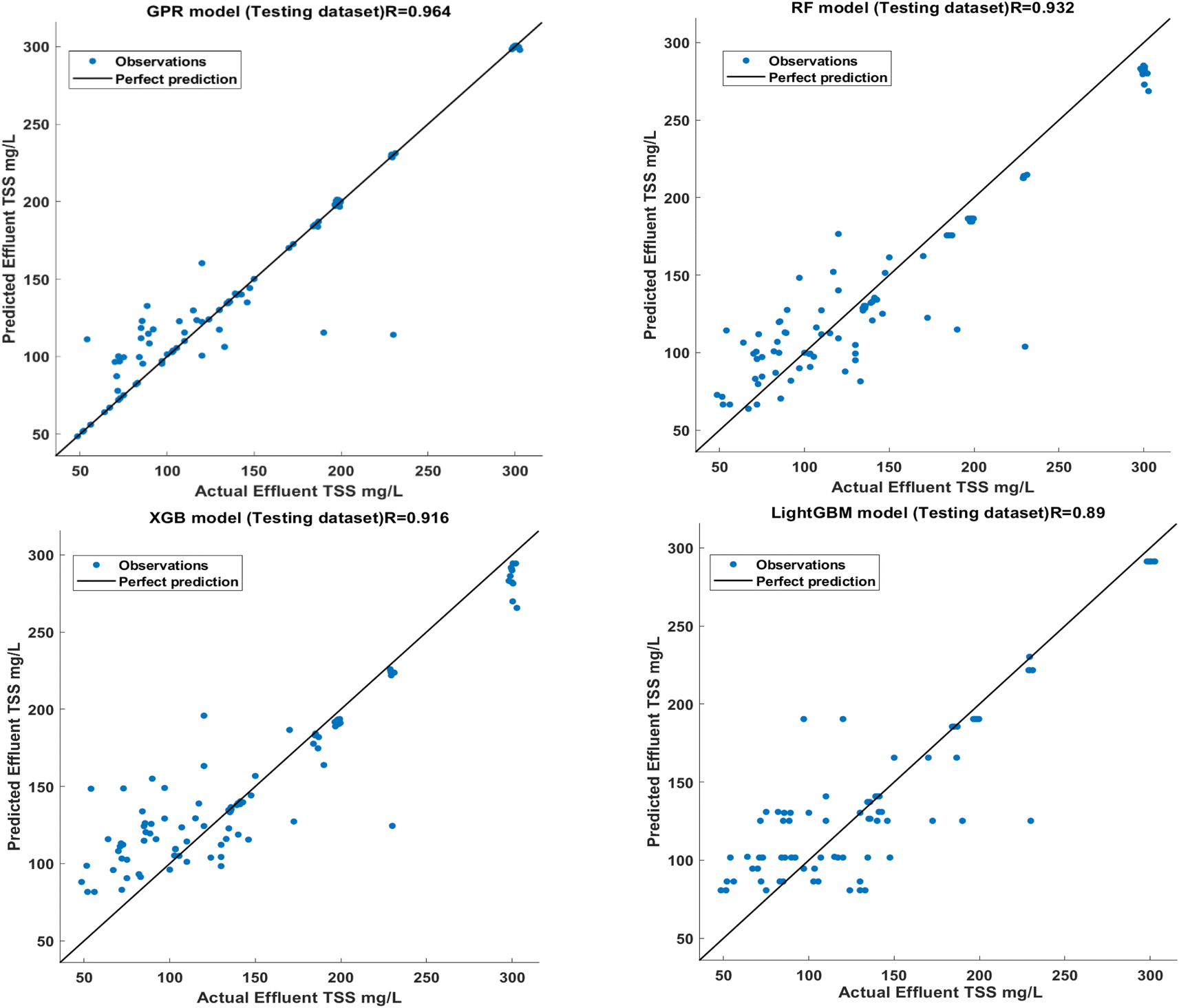Fig. 1 A scatter plot of used ML models for predicting the effluent TSS during the testing phase.

3.2.2 Effluent COD prediction. Table 4 lists the outcomes for the prediction of COD_eff concentration using the training and testing datasets in terms of RMSE, MAE, CC, and MAPE values. Comparison of these figures shows that wastewater treatment plant performance with the altered GPR has somewhat improved [RMSE = (29.61–34.12 mg L⁻¹), MAE = (10.06–14.44), CC = (0.967–0.950) and MAPE = (3.29–5.18%)] as compared to the RF [RMSE = (32.64–44.61 mg L⁻¹), MAE = (4.77–8.52), CC = (0.934–0.806) and MAPE = (4.77–8.52%)], XGB [RMSE = (35.26–46.32 mg L⁻¹), MAE = (17.47–27.74), CC = (0.952–0.901), and MAPE = (5.71–9.96%)] and LightGBM [RMSE = (38.92–48.33 mg L⁻¹), MAE = (23.73–28.94), CC = (0.921–0.891) and MAPE = (7.75–10.39%)]. Based on the results obtained, the GPR model outperformed other regression models such as RF, XGB, and LightGBM in predicting the effluent COD concentration, as indicated in Table 4. Various supervised learning-based algorithms were trained and validated to find the most suitable predictive model for the study. The GPR model showed the highest accuracy in terms of RMSE (29.61 mg L⁻¹), MAE (10.06), CC (0.967), and MAPE (3.29%) during model training, indicating its superior performance over the other models for the given datasets. Additionally, during model testing, the GPR-based prediction model demonstrated better accuracy compared to the other five ML models, with RMSE of 34.12 mg L⁻¹, MAE of 14.44, CC of 0.950, and MAPE of 5.18% (Table 4).

Table 4 Predictive index of COD_eff

Model	RMSE	MAE	CC	MAPE
RF
Training dataset	32.64	14.60	0.956	4.77
Testing dataset	44.61	23.72	0.910	8.52
GPR
Training dataset	29.61	10.06	0.967	3.29
Testing dataset	34.12	14.44	0.950	5.18
XGB
Training dataset	35.26	17.47	0.952	5.71
Testing dataset	46.32	27.74	0.901	9.96
LightGBM
Training dataset	38.92	23.73	0.921	7.75
Testing dataset	48.33	28.94	0.892	10.39

---

To gain a better understanding of the accuracy of the developed models, a scatter plot was generated using the fit line of the best model obtained (Fig. 2). The scatter plot in Fig. 4 displays the predicted effluent COD values of the established models against the test values. It is observed that the GPR model's predicted values are closely aligned with the best-fit line compared to the other models, suggesting the GPR model's suitability. From the figure it can be seen that the performance of GPR is slightly better than RF where these two models showed better performance than XGB and LightGBM. In general, the GPR model agreed well with the real values in the testing stage, while this was not the case for the XGB and LightGBM models. The XGB and LightGBM models attained the weakest performance in the training and testing stages. Based on the attained CC values, the performance of the predictive models in the current study followed the order of GPR > RF > XGB > LightGBM. In contrast to the 2018 study by Hamada et al. 2018, which employed an MLP neural network model to estimate the average monthly wastewater quality indicators at the GWWT plant, our study took a different approach. Hamada's model resulted in an RMSE of 59.48 mg L⁻¹, an R value of 0.754, and an MAPE of 26.29% for predicting COD during testing. Our study focused on predicting wastewater quality indicators one day ahead, employing various techniques, all applied to the same study area. The results we obtained clearly demonstrate that the models we developed outperformed the MLP model used in the earlier study by Hamada et al. This highlights the improved accuracy and performance achieved by our approach in predicting wastewater quality, especially in terms of COD concentration. Furthermore, when we compare our study's predictive capabilities with those of previous works,^52,53 it is evident that our models consistently delivered good and satisfactory results, further emphasizing their effectiveness in enhancing the prediction of effluent COD concentration.

Fig. 2 A scatter plot of ML models for predicting the effluent COD during the testing phase.

3.2.3 Effluent BOD prediction. The results for the prediction of BOD_eff concentration using the training and testing datasets are presented in Table 5 in terms of RMSE, MAE, CC, and MAPE values. These values indicate that the altered GPR slightly improves the performance of the wastewater treatment facility [RMSE = (6.15–13.69 mg L⁻¹), MAE = (3.24–6.41), CC = (0.990–0.975) and MAPE = (2.21–4.72%)] as compared to XGB [RMSE = (9.69–17.76 mg L⁻¹), MAE = (4.81–11.15), CC = (0.973–0.954) and MAPE = (3.29–8.22%)], RF [RSME = (11.35–19.43), MAE = (6.85–14.62), CC = (0.980–0.943), and MAPE = (4.68–10.78%)], and LightGBM [RMSE = (17.70–27.72 mg L⁻¹), MAE = (11.76–19.10), CC = (0.906–0.883) and MAPE = (8.04–14.09%).

Table 5 Predictive index of BOD_eff

Model	RMSE	MAE	R	MAPE
RF
Training dataset	11.35	6.85	0.980	4.68
Testing dataset	19.43	14.62	0.943	10.78
GRP
Training dataset	6.15	3.24	0.990	2.21
Testing dataset	13.69	6.41	0.975	4.72
XGB
Training dataset	9.65	4.81	0.973	3.29
Testing dataset	17.76	11.15	0.954	8.22
LightGBM
Training dataset	17.70	11.76	0.906	8.04
Testing dataset	27.72	19.10	0.883	14.09

---

The results suggest that the GPR model is the most effective regression model, although XGB, and RF also performed well in predicting the effluent BOD concentration. However, the RF and LightGBM algorithms had slightly lower performance compared to the other models (as shown in Table 5). To determine the optimal forecasting model, this study trained and validated supervised learning-based algorithm prediction models (GPR, FR, XGB, and LightGBM). Table 5 indicates that the GPR model achieved the highest accuracy in terms of RMSE (6.15 mg L⁻¹), MAE (3.24), CC (0.990), and MAPE (2.21%), demonstrating that the GPR algorithm is well-suited to the available datasets. Furthermore, during model testing, the GPR-based prediction model exhibited the greatest accuracy in terms of RMSE (13.69 mg L⁻¹), MAE (6.41), CC (0.975), and MAPE (4.72%) in comparison to the other five ML models (Table 5).

To better comprehend the accuracy of the developed models, a scatter plot is made from the best fit line of the best models between the predicted and actual values of BOD_eff concentrations (Fig. 3). Fig. 3 shows the distribution of the produced model's prediction of effluent BOD values in relation to the test values. The developed GPR model's validity is supported by the fact that it is more closely related to the best-fit line than the others. As can be observed from the figure, GPR outperforms XGB and RF, whereas these two models both perform better than LightGBM. The GPR model, in contrast to the LightGBM model, generally agreed well with the real values during the testing stage. In the training and testing phases, it was discovered that the LightGBM model had the worst performance. Based on the obtained CC values, the prediction models in the current study performed in the following order: GPR > XGB > RF > LightGBM. In contrast to Hamada et al. 2018 study, where they used an MLP neural network model to predict the average monthly wastewater quality indicators at the GWWT plant and achieved an RMSE of 29.69 mg L⁻¹, an R-value of 0.78, and an MAPE of 25.45% for BOD predictions during testing, our study took a different approach. Our study focused on predicting wastewater quality indicators one day ahead for the same study area, using alternative methods. The results of our work clearly demonstrate that the models we developed performed better than the MLP model employed in Hamada et al.'s previous research. However, when we compare our study's performance with that of other prior studies,^52,53 it is evident that the predictions for effluent BOD concentration obtained in this study are generally of good and satisfactory quality, strengthening the effectiveness of our approach in improving the accuracy of BOD concentration prediction.

Fig. 3 A scatter plot of ML models for predicting the effluent BOD during the testing phase.

3.3 Sensitivity of input variables

The results of four machine learning models that approximate the best predictive model are further examined in terms of how sensitive the prediction results are to the input parameters. Thus, Fig. 4 shows the sensitivity ranking for the performance of the input parameters from the good obtained predictive models to the TSS, COD and BOD concentrations for the effluent. It shows the importance of the input variables to the model predictions. In the GPR case in prediction of TSS effluent, the temperature and pH were the most important parameters, followed by the BOD influent, COD influent and TSS influent of inflow water. In the GPR case in prediction of COD effluent, the temperature and pH were the most important parameters, followed by the BOD influent, COD influent and TSS influent of inflow water. On the other hand, the three most considerable parameters for the GPR model were temperature, pH, and BOD influent. The most crucial operational variables for bacterial growth at the Gaza wastewater plant's aeration wastewater treatment system are temperature and pH, which could have an impact on how effectively BOD, COD, and TSS are removed from the wastewater.

Fig. 4 Importance of input variables for GPR-based prediction of effluent TSS, COD, and BOD.

As a result, it is acceptable to conclude that temperature and pH are the two factors that have the most impact on machine learning models' ability to forecast the BOD, COD, and TSS contents of effluent. Additionally, the concentrations of BOD, COD, and TSS in the influent were a crucial input factor because they have an immediate impact on the value of BOD, COD, and TSS effluent that is introduced into the wastewater treatment process. Therefore, based on the assessment of characteristics of the treatment process in the Gaza wastewater treatment plant, it could be discovered that the GPR model may lead to a more reasonable model than RF, XGB, and LightGBM. By altering the most physically linked parameters compared to the other ML models, the more reasonable physical relation-based GRP model could be a more dependable model to apply on the avoidance of the high BOD, COD, and TSS concentrations impact management on the system. The highest-ranking parameters of RF, XGB, GPR, and LightGBM were temperature and pH. Machine learning models don't have to express all the physical meaning through the input and output variables, as we can still see this from the results of sensitivity analysis. Moreover, the results of this study's final effect values demonstrated that there was little variation across all variables in RF, XGB, and LightGBM. Compared to the other models utilized in this study for process control, GPR demonstrated outcomes that were more trustworthy and reasonable.

4 Conclusions

The statistical analysis of data shows that the Gaza wastewater treatment plant is not meeting discharge limits, posing a threat to the environment. Despite this, the plant removed 79.32%, 77%, and 77.45% of BOD, COD, and TSS from sewage in 2020 using existing infrastructure. Currently, 80–85% of these pollutants are removed due to reduced wastewater volume and routine maintenance.

Artificial intelligence techniques are an alternative to linear methods. In this research, the capability of GPR, SVM, RF, MLP-NN, XGB and LightGBM methods in the prediction of BOD_eff, COD_eff, and TSS_eff parameters from daily data of the Gaza wastewater treatment plant was evaluated. According to the results, the performance of the GPR model in estimating the daily BOD, COD, and TSS parameters of the effluent quality of the wastewater treatment plant is acceptable according to the RMSE, MAE, MAPE, and CC values of the testing dataset which are (18.28), (7.6), (5.07%) and (0.964) for BOD_eff, (34.12), (14.44), (5.18%) and (0.950) for COD_eff and (13.69), (6.41), (4.72%) and (0.975) for TSS_eff, respectively. The GPR model in predicting TSS_eff, BOD_eff and COD_eff shows better performance than the other models developed during this study. Further sensitivity tests of the effect of the input parameters on the developed ML models were performed for the best network. The following list is provided in order of how each input parameter affects the consequences of the training and testing data for predicting the BOD, COD, and TSS indicators: Temp_inf > pH_inf > BOD_inf > COD_inf > TSS_inf. It is obvious that the temperature and pH parameters have the greatest impact on the developed ML models. However, this study has shown that using machine learning models as early warning systems for water quality control in wastewater treatment could be a reliable approach. To increase the precision of the suggested machine learning models, long-term modeling for the input value sampling may be recommended in the future.

Hamada et al. (2018)²¹ predicted monthly average wastewater indicators at the GWWT plant using an MLP neural network with RMSEs of 29.69, 59.48, and 37.38 mg L⁻¹, R values of 0.784, 0.759, and 0.765, and MAPEs of 25.45%, 26.29%, and 26.33% for BOD, COD, and TSS. In contrast, we used four ML techniques to predict wastewater quality indicators one day ahead for the same study area, and the developed models in this study outperformed the MLP model. Nonetheless, our BOD, COD, and TSS effluent concentration predictions were generally reliable and accurate when compared to previous studies.

Author contributions

Mazan S. Hamada contributed significantly to the allocation of resources for the study, and also contributed to the writing of the original draft and editing process. Hossam Adel Zaqoot conceptualized the study, conducted data analysis, and developed the modeling framework. Also, played a pivotal role in the writing of the original draft, and actively participated in the editing process. Waqar Ahmed Sethar conducted data analysis and contributed to the modeling aspect of the study.

Conflicts of interest

The authors declare no conflict of interest.

Acknowledgements

The authors gratefully acknowledge the Palestinian Water Authority, Gaza Municipality, and Coastal Municipalities Water Utility for providing the wastewater quality datasets required to complete this research.

References

1. A. L. Abrams, K. Carden, C. Teta and K. Wagsæther, Water, sanitation, and hygiene vulnerability among rural areas and small towns in South Africa: exploring the role of climate change, marginalization, and inequality, Water, 2021, 13, 2810.
2. N. Julio, R. Figueroa and R. D. Ponce Oliva, Water resources and governance approaches: insights for achieving water security, Water, 2021, 13, 3063.
3. M. A. Shannon, P. W. Bohn, M. Elimelech, J. G. Georgiadis, B. J. Mariñas and A. M. Mayes, Science and technology for water purification in the coming decades, Nature, 2008, 452, 301–310.
4. M. Zhou, Y. Zhang, J. Wang, Y. Shi and V. Puig, Water Quality Indicator Interval Prediction in Wastewater Treatment Process Based on the Improved BES-LSSVM Algorithm, Sensors, 2022, 22, 422,  DOI:10.3390/s22020422.
5. J. Qiao, L. Wang, C. Yang and K. Gu, Adaptive Levenberg-Marquardt algorithm-based echo state network for Chaotic time series prediction, IEEE Access, 2018, 6, 10720–10732.
6. Y. Chen and D. Han, Water quality monitoring in smart city: a pilot project, Autom. Constr., 2018, 89, 307–316,  DOI:10.1016/j.autcon.2018.02.008.
7. Z. Liu, J. Wan, Y. Ma and Y. Wang, Online prediction of effluent COD in the anaerobic wastewater treatment system based on PCA-LSSVM algorithm, Environ. Sci. Pollut. Res., 2019, 26, 12828–12841.
8. I. S. Baruch, P. Georgieva, J. Barrera-Cortes and S. Feyo de Azevedo, Adaptive recurrent neural network control of biological wastewater treatment, Int. J. Smart Sens. Intell. Syst., 2005, 20(2), 173–193.
9. A. Manandhar, A. Fischer, D. J. Bradley, M. Salehin, M. S. Islam, R. Hope and D. A. Clifton, Machine learning to evaluate impacts of flood protection in Bangladesh, 1983–2014, Water, 2020, 12(2), 483,  DOI:10.3390/w12020483.
10. H. Liu, H. Zhang, Y. Zhang, F. Zhang and M. Huang, Modeling of Wastewater Treatment Processes Using Dynamic Bayesian Networks Based on Fuzzy PLS, IEEE Access, 2020, 8, 92129–92140.
11. H. Lu and X. Ma, Hybrid decision tree-based machine learning models for short-term water quality prediction, Chemosphere, 2020, 249, 126169.
12. P. Zhou, Z. Li, S. Snowling, B. W. Baetz, D. Na and G. Boyd, A random forest model for inflow prediction at wastewater treatment plants, Stoch. Environ. Res. Risk Assess., 2019, 33, 1781–1792.
13. A. G. Capodaglio, H. V. Jones, V. Novotny and X. Feng, Sludge bulking analysis and forecasting: application of system identification and artificial neural computing technologies, Water Res., 1991, 25(10), 1217–1224.
14. J. F. Qiao, G. T. Han, H. G. Han, C. L. Yang and W. Li, Decoupling control for wastewater treatment process based on recurrent fuzzy neural network, Asian J. Control, 2019, 21(3), 1270–1280.
15. A. Dairi, T. Cheng, F. Harrou, Y. Sun and T. Leiknes, Deep learning approach for sustainable WWTP operation: a case study on data-driven influent conditions monitoring, Sustain. Cities Soc., 2019, 50, 101670.
16. B. Mamandipoor, M. Majd, S. Sheikhalishahi, C. Modena and V. Osmani, Monitoring and detecting faults in wastewater treatment plants using deep learning, Environ. Monit. Assess., 2020, 192(2), 148.
17. Z. Wang, Y. Man, Y. Hu, J. Li, M. Hong and P. Cui, A deep learning based dynamic COD prediction model for urban sewage, Environ. Sci.: Water Res. Technol., 2019, 5(12), 2210–2218.
18. I. Pisa, I. Santın, I. L. Vicario, A. Morell and R. Vilanova, A Recurrent Neural Network for Wastewater Treatment Plant effluents’ prediction, Actas Jorn. Geol. Argent., 2018 DOI:10.17979/spudc.9788497497565.0621.
19. J. F. de Canete, P. D. S. Orozco, R. Baratti, M. Mulas, A. Ruano and A. Garcia-Cerezo, Soft-sensing estimation of plant effluent concentrations in a biological wastewater treatment plant using an optimal neural network, Expert Syst. Appl., 2016, 63, 8–19.
20. Q. Cong and W. Yu, Integrated soft sensor with wavelet neural network and adaptive weighted fusion for water quality estimation in wastewater treatment process, Measurement, 2018, 124, 436–446.
21. M. Hamada, H. A. Zaqoot and A. Abu Jreiban, Application of artificial neural networks for the prediction of Gaza wastewater treatment plant performance–Gaza Strip, J. Appl. Res. Water Wastewater, 2018, 5(1), 399–406,  DOI:10.22126/arww.2018.874.
22. M. Zeinolabedini and M. Najafzadeh, Comparative study of different wavelet-based neural network models to predict sewage sludge quantity in wastewater treatment plant, Environ. Monit. Assess., 2019, 191, 1–25.
23. A. Kadam, V. Wagh, A. Muley, B. Umrikar and R. Sankhua, Prediction of water quality index using artificial neural network and multiple linear regression modelling approach in Shivganga River basin, India, Model. Earth Syst. Environ., 2019, 5, 951–962.
24. S. Heddam, H. Lamda and S. Filali, Predicting effluent biochemical oxygen demand in a wastewater treatment plant using generalized regression neural network-based approach: a comparative study, Environ. Processes, 2016, 3, 153–165.
25. V. Nourani, G. Elkiran and S. I. Abba, Wastewater treatment plant performance analysis using artificial intelligence—an ensemble approach, Water Sci. Technol., 2018, 78, 2064–2076.
26. T. Cheng, A. Dairi, F. Harrou, Y. Sun and T. Leiknes, Monitoring influent conditions of wastewater treatment plants by nonlinear data-based techniques, IEEE Access, 2019, 7, 108827–108837.
27. H. Han, H. Liu, Z. Liu and J. Qiao, Fault detection of sludge bulking using a self-organizing type-2 fuzzy-neural-network, Control Eng. Pract., 2019, 90, 27–37.
28. J. Wu, H. Cheng, Y. Liu, B. Liu and D. Huang, Modeling of adaptive multi-output soft-sensors with applications in wastewater treatments, IEEE Access, 2019, 7, 161887–161898.
29. K. Lotfi, H. Bonakdari, I. Ebtehaj, F. S. Mjalli, M. Zeynoddin, R. Delatolla and B. Gharabaghi, Predicting wastewater treatment plant quality parameters using a novel hybrid linear-nonlinear methodology, J. Environ. Manage., 2019, 240, 463–474.
30. H. Han, L. Zhang and J. Qiao, Data-based predictive control for wastewater treatment process, IEEE Access, 2017, 6, 1498–1512.
31. D. Ribeiro, A. Sanfins and O. Belo, Wastewater Treatment Plant Performance Prediction with Support Vector Machines, in Advances in Data Mining, Applications and Theoretical Aspects, Springer, Berlin/Heidelberg, Germany, 2013, pp. 99–111.
32. V. Mateo Pérez, J. M. Mesa Fernández, F. Ortega Fernández and J. Villanueva Balsera, Gross Solids Content Prediction in Urban WWTPs Using SVM, Water, 2021, 13, 442.
33. A. Baghban, J. Sasanipour, S. Habibzadeh and Z. Zhang, Sulfur dioxide solubility prediction in ionic liquids by a group contribution—LSSVM model, Chem. Eng. Res. Des., 2019, 142, 44–52.
34. P. G. Nieto, E. García Gonzalo, G. Arbat, M. Duran Ros, F. R. de Cartagena and J. Puig Bargues, A new predictive model for the filtered volume and outlet parameters in micro-irrigation sand filters fed with effluents using the hybrid PSO-SVM-based approach, Comput. Electron. Agric., 2016, 125, 74–80.
35. S. Chen, G. Fang, X. Huang and Y. Zhang, Water quality prediction model of a water diversion project based on the improved artificial bee colony–backpropagation neural network, Water, 2018, 10, 806,  DOI:10.3390/w10060806.
36. W. Yao, Z. Zeng and C. Lian, Generating probabilistic predictions using mean-variance estimation and echo state network, Neurocomputing, 2017, 219, 536–547.
37. A. M. Aish, H. A. Zaqoot and S. M. Abdeljawad, Artificial neural network approach for predicting reverse osmosis desalination plants performance in the Gaza Strip, Desalination, 2015, 367, 240–247.
38. Palestinian Central Bureau of Statistics (PCBS), About 13 million Palestinians in the historical Palestine and diaspora, on the occasion of the international population day 11/7/2019, 2021, https://www.pcbs.gov.ps/post.aspx?lang=en%26ItemID=3503, accessed on 20/06/2022.
39. H. Al-Najjar, G. Ceribasib and A. I. Ceyhunlub, Effect of unconventional water resources interventions on the management of Gaza coastal aquifer in Palestine, Water Supply, 2021, 21(8), 4205,  DOI:10.2166/ws.2021.170.
40. F. R. Saen, The use of artificial neural networks for technology selection in the presence of both continuous and categorical data, World Appl. Sci. J., 2009, 6, 1177–1189.
41. U. Ahmed, R. Mumtaz, H. Anwar, A. A. Shah, R. Irfan and J. García-Nieto, Efficient water quality prediction using supervised Machine Learning, Water, 2019, 11(11), 2210,  DOI:10.3390/w11112210.
42. S. Badillo, B. Banfai, F. Iakov, I. Davydov, L. L. Hutchinson, T. Kam-Thong, J. Siebourg-Polster, B. Steiert and J. D. Zhang, An Introduction to Machine Learning, Clin. Pharmacol. Ther., 2020, 107(4), 871–885,  DOI:10.1002/cpt.1796.
43. H. Tyralis, G. Papacharalampous and A. Langousis, A Brief Review of Random Forests for Water Scientists and Practitioners and Their Recent History in Water Resources, Water, 2019, 11, 910,  DOI:10.3390/w11050910.
44. T. Hastie, R. Tibshirani and J. Friedman, The Elements of Statistical Learning, Springer-Verlag, New York, NY, USA, 2nd edn, 2009.
45. T. Chen and C. Guestrin, XGBoost: A Scalable Tree Boosting System, San Francisco, CA, USA, 2016.
46. S. K. Bhagat, T. Tiyasha, T. M. Tung, R. Mostafa and Z. M. Yaseen, Manganese (Mn) removal prediction using extreme gradient model, Ecotoxicol. Environ. Saf., 2020, 204, 111059,  DOI:10.1016/j.ecoenv.2020.111059.
47. F. Pedregosa, G. Varoquaux, A. Gramfort, V. I. Michel, B. Thirion, O. Grisel, M. Blondel, P. Prettenhofer, R. Weiss, V. Dubourg, J. Vanderplas, A. Passos, D. Cournapeau, M. Brucher, M. Perrot and E. Duchesnay, Scikit-learn: Machine learning in Python, J. Mach. Learn. Res., 2011, 12, 2825–2830.
48. X. Fang, Z. Zhai, J. Zang and Y. Zhu, An Intelligent Dosing Algorithm Model for Wastewater Treatment Plan, J. Phys.: Conf. Ser., 2022, 2224, 012027,  DOI:10.1088/1742-6596/2224/1/012027.
49. A. Alsulaili and A. Refaie, Artificial neural network modeling approach for the prediction of five-day biological oxygen demand and wastewater treatment plant performance, Water Supply, 2021, 21(5), 1861–1877.
50. S. Singha, S. Pasupuleti, S. S. Singha, R. Singh and S. Kumar, Prediction of groundwater quality using efficient machine learning technique, Chemosphere, 2021, 276, 130265.
51. S. Tertouche, S. Bellebia, Z. Bengharez, Z. Zian and S. Jellali, Performance Assessment of Wastewater Treatment Plants (WWTPs) and Application of Electrocoagulation Process to Improve Their Operation, Pol. J. Environ. Stud., 2021, 30(6), 5273–5284,  DOI:10.15244/pjoes/134084.
52. F. Granata, G. Esposito, R. Gargano and G. de Marinis, Machine Learning Algorithms for the Forecasting of Wastewater Quality Indicators, Water, 2017, 9, 105,  DOI:10.3390/w9020105.
53. M. T. Aalami, N. Hejabi, V. Nourani and S. M. Saghebian, Investigation of Artificial Intelligence Approaches Capability in Predicting the Wastewater Treatment Plant Performance (Case Study: Tabriz Wastewater Treatment Plant), Amirkabir J., Civ. Eng., 2019, 53(3), 235–238,  DOI:10.22060/ceej.2019.16757.6334.

---