
 Open Access Article
 This Open Access Article is licensed under a
 Creative Commons Attribution 3.0 Unported Licence
Emergent mesoscale correlations in active solids with noisy chiral dynamics†
Amir
Shee
 a,
Silke
Henkes
*b and
Cristián
Huepe
*acd
a,
Silke
Henkes
*b and
Cristián
Huepe
*acd
aNorthwestern Institute on Complex Systems and ESAM, Northwestern University, Evanston, IL 60208, USA
bLorentz Institute for Theoretical Physics, LION, Leiden University, P.O. Box 9504, 2300 RA Leiden, The Netherlands. E-mail: shenkes@lorentz.leidenuniv.nl
cSchool of Systems Science, Beijing Normal University, Beijing, People's Republic of China
dCHuepe Labs, 2713 West August Blvd #1, Chicago, IL 60622, USA. E-mail: cristian@northwestern.edu
First published on 18th September 2024
Abstract
We present the linear response theory for an elastic solid composed of active Brownian particles with intrinsic individual chirality, deriving both a normal mode formulation and a continuum elastic formulation. Using this theory, we compute analytically the velocity correlations and energy spectra under different conditions, showing an excellent agreement with simulations. We generate the corresponding phase diagram, identifying chiral and achiral disordered regimes (for high chirality or noise levels), as well as chiral and achiral states with mesoscopic-range order (for low chirality and noise). The chiral ordered states display mesoscopic spatial correlations and oscillating time correlations, but no wave propagation. In the high chirality regime, we find a peak in the elastic energy spectrum that leads to a non-monotonic behavior with increasing noise strength that is consistent with the emergence of the ‘hammering state’ recently identified in chiral glasses. Finally, we show numerically that our theory, despite its linear response nature, can be applied beyond the idealized homogeneous solid assumed in our derivations. Indeed, by increasing the level of activity, we show that it remains a good approximation of the system dynamics until just below the melting transition. In addition, we show that there is still an excellent agreement between our analytical results and simulations when we extend our results to heterogeneous solids composed of mixtures of active particles with different intrinsic chirality and noise levels. The derived linear response theory is therefore robust and applicable to a broad range of real-world active systems. Our work provides a thorough analytical and numerical description of the emergent states in a densely packed system of chiral self-propelled Brownian disks, thus allowing a detailed understanding of the phases and dynamics identified in a minimal chiral active system.
1 Introduction
Chirality is a fundamental property of most chemical, physical, and biological systems that is expected to naturally occur in active matter. Indeed, in the context of self-propelled particles, chiral motion has been shown to spontaneously arise due to asymmetries in the self-propulsion forces or in the particle geometry,1–4 or as a result of interactions with external fields.5,6The relationship between activity and chirality has been considered in multiple contexts. Chiral motion has been observed experimentally in active biomolecules7 such as proteins,8 in microtubules,9 and in single cells, including bacteria10–12 and sperm cells.13,14 It has been studied theoretically for single circle swimmers,15–23 for the clockwise circular dynamics of E. coli,24,25 and for circular and helical motion under chemical gradients.26,27 Groups of chiral swimmers have been shown to display unique forms of collective dynamics, whether chirality resulted from shape asymmetry,28–32 mass distribution,33 or catalysis coating.34 Chiral particles can also display a range of non-equilibrium phases, including a gas of spinners and aster-like vortices, rotating flocks with either polar or nematic alignment,32 and states displaying phase separation, swarming, or oscillations, among others.35
Several theoretical studies have shown that chirality can strongly affect the collective states that are typically found in achiral active systems. In cases with explicit mutual alignment interactions (as in the Vicsek model), it has been shown that chiral polar swimmers display stronger flocking behavior than achiral ones, with higher levels of polarization in the ordered phase,36 and that large rotating clusters with enhanced size and shape fluctuations can emerge.37 In cases with other types of angular interactions, a marked attenuation of motility-induced phase separation (MIPS),38 the emergence of vortex arrays,39 and chirality-triggered oscillatory dynamic clustering40 have been observed. Chirality has also been found to affect the collective states of active particles without explicit alignment interactions. For instance, chiral active Brownian particles can suppress conventional MIPS due to the formation of dynamical clusters that disrupt the MIPS clusters,41,42 and a quantitative field theory was developed to account for this suppression.43 Furthermore, chiral active particles with fast rotation have been found to form non-equilibrium hyperuniform fluids.44,45
Novel collective states have also been identified in inhomogeneous systems that combine different types of activity and chirality. For example, in a low-density environment, binary mixtures of passive and active chiral self-propelled particles exhibit transitions from mixed gels to rotating passive clusters, and then to homogeneous fluids.46 In addition, a mixture of active particles with different chirality frequencies can create complex combinations of clusters of different sizes, rotating at different rates.47 At low density, active chiral mixtures with opposite chiralities can also give rise to spontaneous demixing.48 Moreover, the combination of chiral and achiral swarming coupled oscillators leads to a range of novel behaviors, such as the formation of vortex lattices, pulsating clusters, or interacting phase waves.49
Although most research on chiral systems has focused on liquid- and gas-like states, solid chiral active states have been found to naturally arise in systems such as groups of spinning magnetic particles50 or of starfish oocytes51 when hydrodynamic torque couplings are included, resulting in active chiral crystals.51–57 The interactions in these cases can be cast as nonreciprocal odd-elastic viscous active couplings, to place them within the framework of odd active matter.58 The elastic coefficients then acquire non-symmetric contributions, and the resulting lack of energy conservation, as well as the polarity-position coupling, allow for wave propagation and work cycles. Here we will consider a different class of systems, focusing on a minimal model of solid “dry” active matter, where chirality is introduced as part of the active forces, not as an active stress. Since in this case there are no action–reaction effects in the active driving, activity cannot be recast as part of the stress tensor or in the elastic coefficients, and an odd-elasticity framework is not applicable.
Solid and dense active systems without chirality have received significant interest in recent years. On one hand, the emergent states of self-propelled particles with self-alignment interactions have been studied in multiple contexts.59–64 On the other hand, various dense and glassy active matter systems65–68 without any alignment interaction have been described theoretically, using active Brownian particles in ref. 69–81 and active Ornstein–Uhlenbeck particles in ref. 82–88. However, their chiral counterparts have so far received limited attention. In one study, Debets et al.89 examined the glassy dynamics of chiral active Brownian particles, showing that they exhibit highly nontrivial states and a non-monotonic behavior of the diffusion constant versus noise at high chirality that we also find in our system. In another study, Caprini et al.90 showed the emergence of rotating and oscillating states, deriving an analytical phase diagram by applying an active solid approach similar to that presented below, but in a different context. Lastly, in recent work, Kuroda et al.91 used linear elasticity theory to deduce the presence of long-range translational order in active chiral crystals with zero noise.
In this paper, we investigate the collective dynamics of chiral active Brownian disks with elastic repulsive interactions at high densities, in the solid state. We identify and describe the different phases, finding an emergent mesoscopic length scale that can display or not oscillatory time correlations, depending on the ratio of chiral motion to rotational noise. We derive an analytical active solid theory to describe these phases, using a normal mode approach and a continuum elasticity approach, both of which match our simulations. In addition, we show that these results remain valid well into the nonlinear regime, just below the melting transition, and inform the dynamics of the fluid state. They also extend to different kinds of active binary mixtures, including mixtures of chiral and achiral particles, of chiral particles with different rotational speeds, and of chiral particles with different levels of rotational diffusion.
The paper is organized as follows. In Section 2, we describe our two-dimensional active solid model of densely packed self-propelled disks with elastic interactions and intrinsic individual chirality. In Section 3, we overview the phase space of dynamical regimes as a function of chirality and rotational diffusion. In Section 4, we present our analytical results. We first calculate the orientation autocorrelation functions using a Fokker–Planck approach; then describe the normal mode formalism for active solids, calculating the average energy per mode and the spatial velocity correlations; and finally describe the continuum elastic formulation. In Section 5, we characterize the dynamics described by our results and compare them to simulations. In Section 6, we examine the melting regime by increasing the level of activity. In Section 7, we extend our results to heterogeneous mixtures of disks with different levels of activity and chirality. Finally, Section 8 presents our conclusions.
2 Model
We consider a system of N densely packed soft chiral self-propelled disks following overdamped dynamics in a two dimensional periodic box of size L × L. Disregarding passive translational diffusion, the dynamics of the position ri ≡ (xi,yi) and of the heading direction or orientational unit vector![[n with combining circumflex]](https://www.rsc.org/images/entities/i_char_006e_0302.gif) i ≡ (cos(θi),sin(θi)) of the i-th disk will be given by
i ≡ (cos(θi),sin(θi)) of the i-th disk will be given by| ṙi = v0i + μFi, | (1) |
 | (2) |
⊥i is a unit vector perpendicular to i. Noise is introduced through the random variable ηi(t), following Gaussian white noise with 〈ηi(t)〉 = 0 and 〈ηi(t)ηj(t′)〉 = δijδ(t − t′). The sum of all contact forces over disk i is  , where Si is the set of indexes of all disks that overlap disk i. These forces are modeled as linear repulsion, with fij = k(|rij| − l0)rij/|rij| if |rij| ≤ l0 and fij = 0 otherwise, were rij = rj − ri and l0 = 2r0 is the equilibrium center-to-center distance between two neighboring disks of radius r0. We note that, in real-world scenarios, Ω and Dr cannot be exactly the same for all disks. In Section 7, we thus conduct a comprehensive investigation into binary and complex mixtures of disks with different Dr and Ω values, substituting Dr by Dir and Ω by Ωi in eqn (2).
We note that the orientation dynamics in eqn (2) are decoupled from the position dynamics in eqn (1), and result from the interplay between deterministic chirality and angular diffusion. The deterministic angular speed Ω sets a rotational timescale τΩ = Ω−1; the diffusion constant Dr sets a persistence timescale τr = Dr−1. We will show below that the interplay between rotational, persistence, and elastic timescales can generate different collective states.
3 State space overview
We begin by characterizing the different regimes that can be reached by the model introduced above. Fig. 1(a) presents a diagram of the resulting phases as a function of the chiral angular speed Ω and the angular diffusion coefficient Dr, with the boundaries computed analytically as we will detail in Section 4. Broadly speaking, the system develops mesoscopic range order for low enough Ω and Dr values (below the blue line), where patches of disks with strong velocity correlations spontaneously appear at different scales. For high Ω/Dr ratios (above the red line) the velocity directions displayed by these patches rotate with a clearly defined chirality, determined by Ω, defining the chiral mesoscopic range order (CMRO) regime. For low Ω/Dr ratios, no clear chirality is observed and we define the mesoscopic range order (MRO) regime. In the high Ω and high Dr regimes (beyond the blue line), we find instead no extended regions of high velocity correlation. The individual particle motion is dominated by deterministic chiral rotation for high Ω/Dr ratios (above the red line), in the chiral disorder (CD) regime, and by stochastic rotational diffusion for low Ω/Dr ratios (below the red line), in the dynamic disorder (DD) regime. Note that the transitions between the four regimes are smooth and determined by the spatiotemporal dynamics.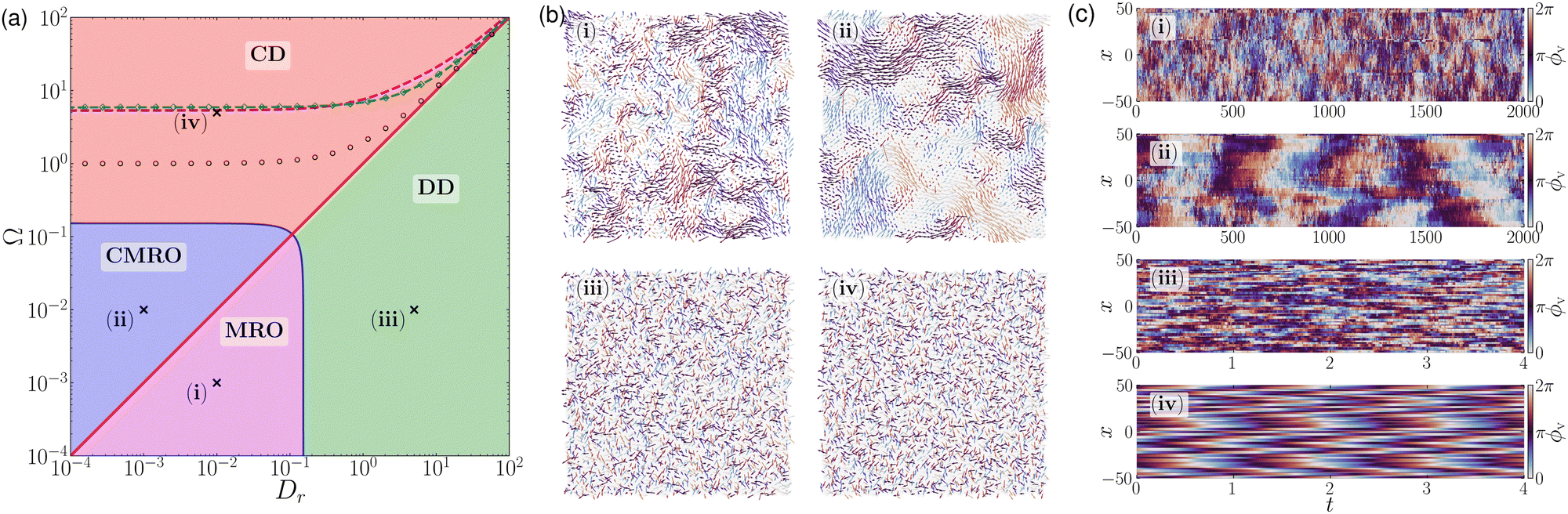 | ||
| Fig. 1 Dynamical regimes and collective states identified in an active solid with noisy chiral dynamics. (a) Phases on the Dr − Ω plane: mesoscopic range order (MRO), chiral mesoscopic range order (CMRO), dynamic disorder (DD), and chiral disorder (CD). The red line traces Dr = Ω, separating the chiral (Dr < Ω) and achiral (Dr ≥ Ω) regimes. The blue line represents ξT = l0, where l0 is the equilibrium distance between neighboring particles. The dashed green line and open green diamonds trace two analytical approximations of the maxima of the elastic energy. The magenta dashed line shows an analytical expression for the minima of the mean-squared velocity, and thus also of the kinetic energy. The black open circles curve provides the analytical result for the maximum of the steady-state mean-squared displacement of a single particle in a harmonic well (see Appendix B). (b) Snapshots of simulations in the four regimes: (i) MRO, (ii) CMRO, (iii) DD, and (iv) CD. Each arrow is colored by angle and represents the direction and magnitude of the velocity vector of the disc at its location. (c) Kymographs corresponding to the snapshots, depicting space-time plots of the velocity angles obtained from simulations, following the dynamics in time of a slice of the system along the x direction. The snapshots and kymographs display results of simulations performed with the parameter combinations indicated by crosses in the phase diagram in panel (a). | ||
Fig. 1(b) and (c) present snapshots of the velocity vectors and kymographs, respectively, describing the spatiotemporal dynamics of the velocity angles, for simulations in each one of the four regimes. Here the sub-panels correspond to: (i) the MRO regime for Dr = 10−2, Ω = 10−3, see ESI,† (ref. 92) Movie S1;92 (ii) the CMRO regime for Dr = 10−3, Ω = 10−2, see Movie S2 (ESI†);92 (iii) the DD regime for Dr = 5, Ω = 10−2, see Movie S3 (ESI†);92 and (iv) the CD regime for Dr = 10−2, Ω = 5, see Movie S4 (ESI†).92
All simulations were carried out for N = 3183 disks of radius r0 = 1 in a periodic square box of side L = 100, which results in a packing fraction of ϕ = Nπr02/L2 ≈ 1, and for the following simulation parameters (unless otherwise stated): mobility μ = 1, elastic repulsive strength k = 1, and active speed v0 = 0.01. The simulations were performed at sufficiently high density and low active speed to avoid melting, phase separation, and clustering, in order to focus on the linear response regime. Spatially, the disks form a crystalline triangular packings without defects, well in the solid phase, without rearrangements for the duration of the simulation. In the snapshots, each disk is represented by a small arrow starting at ri, pointing towards ṙi, with length proportional to ‖ṙi‖, and colored by angle. In the kymographs, we use colors to display the angle of the velocity ṙi of all disks located within a narrow slit, with −r0 ≤ y ≤ + r0, as a function of their x position and time.
The snapshots in sub-panels (i) and (ii) of Fig. 1(b) clearly show the emergence of mesoscopic-range order, while the kymographs in sub-panels (i) and (ii) of Fig. 1(c) show that their temporal dynamics is distinct, with only sub-panel (ii) showing periodic dynamics that result from a close to deterministic local rotation of the i vector. Correspondingly, the snapshots in sub-panels (iii) and (iv) of Fig. 1(b) show disordered states, while the kymographs in sub-panels (iii) and (iv) of Fig. 1(c) show that the dynamics in the DD regime is random in time while the CD regime dynamics is quasiperiodic. Note that the periodicity of the angular dynamics in sub-panels (ii) and (iv) of Fig. 1(c) matches the expected full rotation period T = 2π/Ω, with T = 200π ≃ 628.32 for (ii) and T = 2π/5 ≃ 1.26 for (iv).
In addition to the four regimes described above, the diagram in Fig. 1(a) also contains dashed green and magenta lines, as well as lines of open black circles and green diamonds. These trace four different analytical approximations for the location in the diagram of the ‘hammering state’ identified in ref. 89, where the elastic energy contained by the system is maximal and its kinetic energy is minimal (see ESI,† (ref. 92) Movie S592 for a simulation with Dr = Ω = 10).
We will deduce analytically below the dynamics and boundaries of the different regimes described above.
4 Analytical results
In this section, we present the analytical formulations used to describe the system. We begin by computing the orientation dynamics of the heading direction in Section A, since they are not coupled to the positions. We then formulate a linear response theory, adopting the method in Henkes et al.93 to describe the linear response in terms of normal modes in Section B, to then calculate the energy per mode and spatial velocity correlations. We further simplify the analytical description by implementing a continuum elasticity framework in Section C, to compute mean-squared velocity and velocity autocorrelation functions.4.1 Orientation dynamics
Given that the orientation evolves independently in eqn (2), the probability distribution P(,t) for the heading direction as a function of time will follow the Fokker–Planck equation| ∂tP(,t) = Dr∇2P − Ω⊥·∇P, | (3) |
is the Laplacian in orientation space. Using a Laplace transformation approach described in detail in Appendix A, we can compute an exact expression for the heading orientation autocorrelation, which is given by〈(t)·(0)〉 = e−Drt![[thin space (1/6-em)]](https://www.rsc.org/images/entities/char_2009.gif) cos(Ωt). cos(Ωt). | (4) |
Here, the decay rate of the exponential term is given by τr = Dr−1 and the period of chiral rotation, by τΩ = Ω−1. We thus define Dr = Ω as the critical line between a regime dominated by the angular noise and a regime dominated by the deterministic chirality, which we highlighted as the red diagonal line in Fig. 1(a). Note that this boundary is formally analogous in eqn (4) to the limit between damped and overdamped oscillations, where the high angular diffusion case corresponds to the overdamped regime, as the mean temporal heading correlations display no oscillatory component.
4.2 Normal mode formulation
In order to express the dynamics in terms of the normal modes of vibration of the passive system, we first define as r0i the equilibrium position of disk i for v0 = 0, which corresponds to a minimum of the elastic energy. Using eqn (1), we then find that the dynamics of small displacements δri = ri − r0i around these equilibrium positions are described by | (5) |
![[Doublestruck K]](https://www.rsc.org/images/entities/char_e16e.gif) ij corresponds to a 2 × 2 block of the 2N × 2N dynamical matrix. We are interested in expressing the dynamics over the normal elastic modes of the system, i.e., over the eigenvectors of the dynamical matrix. Each of these 2N normal modes corresponds to a 2N-dimensional eigenvector that can be written as a list of N two-dimensional vectors, given by (ξν1,…,ξνN), where ν = 1,…,2N labels the eigenvector mode associated to the eigenvalue λν.
ij corresponds to a 2 × 2 block of the 2N × 2N dynamical matrix. We are interested in expressing the dynamics over the normal elastic modes of the system, i.e., over the eigenvectors of the dynamical matrix. Each of these 2N normal modes corresponds to a 2N-dimensional eigenvector that can be written as a list of N two-dimensional vectors, given by (ξν1,…,ξνN), where ν = 1,…,2N labels the eigenvector mode associated to the eigenvalue λν.
We can formally write the displacements in terms of the eigenmodes described above as 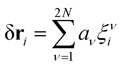 . Projecting eqn (5) onto the normal modes, we then obtain the following uncoupled equations for the dynamics of the normal mode amplitudes:
| ȧν = ην − λνaν, | (6) |
 | (7) |
i. The central limit theorem then implies that ην must follow a Gaussian distribution, here with 〈ην(t)〉 = 0. Additionally, since the eigenvectors form an orthonormal basis where 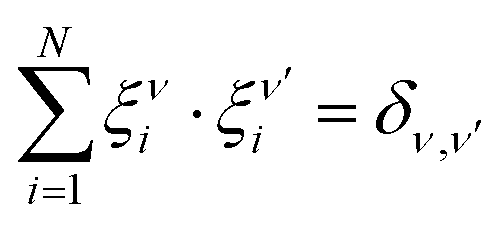 , the corresponding two-time correlation function will be given by 〈ην(t)ην′(t′)〉 = (v02/2)〈(t)·(t′)〉δν,ν′. Replacing the heading autocorrelation expression in eqn (4), we finally obtain 〈ην(t)ην(0)〉 = (v02/2)e−Drtcos(Ωt), which implies that the statistical properties of the noise ην are the same for any mode ν.
We now calculate the mean potential energy stored in each mode (see ESI,† (ref. 92) Section SII for details). By solving eqn (6), we first find
 | (8) |
 to obtain
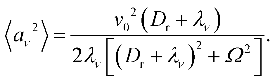 | (9) |
 | (10) |
 , corresponding to the dominant mode, i.e. the maximum eigenvalue λmax = 5.93 ± 0.01. This curve is displayed as the open green diamonds in Fig. 1(a).
In Fig. 2(c), we visualize a color map of the energy  on the Dr − Ω plane that clearly shows an increase of elastic energy in the low Dr and low Ω regimes. Fig. 2(e) presents E/Nv02 as function of Dr for three different Ω = 1, 10, 20 values, showing the presence of a maximum at intermediate Dr noise strengths, for high chirality (Ω = 10, 20). In this regime, we thus find that the elastic energy can grow despite an increase in noise strength. In Fig. 2(g), we plot E/Nv02 as function of Ω for three different Dr = 1, 10, 20 values, showing a monotonic decrease of the elastic energy. We display the maximum of E/Nv02 in the Dr − Ω plane as the dashed green line in Fig. 1(a), which matches the previously computed
  curve. This curve suggests that an increase in elastic energy with noise strength indicates the presence of the ‘hammering state’.89
 | ||
Fig. 2 Analytical features of the characteristic length scales, energy, and mean-squared velocity in an active solid with noisy chiral dynamics. (a) and (b) Color maps of the longitudinal ξL and transverse ξT characteristic length scales on the Dr − Ω plane, respectively, computed using the continuum elastic formulation in eqn (19). (c) Color map of the energy  on the Dr − Ω plane, as derived from the normal mode formulation in eqn (10). (d) Color map of the mean-squared velocity 〈|v|2〉/v02 on the Dr − Ω plane, resulting from the continuum elastic formulation in eqn (20). (e) and (f) Plot of E/Nv02 and of 〈|v|2〉/v02, respectively, as a function of Dr, for Ω = 1, 10, 20. The inset zooms into the minimum of 〈|v|2〉/v02 that appears at high Ω values. (g) and (h) Plot of E/Nv02 and of 〈|v|2〉/v02, respectively, as a function of Ω, for Dr = 1, 10, 20. on the Dr − Ω plane, as derived from the normal mode formulation in eqn (10). (d) Color map of the mean-squared velocity 〈|v|2〉/v02 on the Dr − Ω plane, resulting from the continuum elastic formulation in eqn (20). (e) and (f) Plot of E/Nv02 and of 〈|v|2〉/v02, respectively, as a function of Dr, for Ω = 1, 10, 20. The inset zooms into the minimum of 〈|v|2〉/v02 that appears at high Ω values. (g) and (h) Plot of E/Nv02 and of 〈|v|2〉/v02, respectively, as a function of Ω, for Dr = 1, 10, 20. | ||
Eqn (10) also provides us with expressions for the low and high limits of angular noise or chirality. In the high noise case, Dr/λν ≫ 1 and the mean energy per mode reduces to Eν ≈ v02Dr/4(Dr2 + Ω2), which gives rise to two limits: (i) a low chirality limit Ω → 0, where Eν → v02/4Dr, and (ii) a high chirality limit Ω → ∞, where Eν → 0. This latter limit is connected to the fact that very high chirality disrupts the persistent translation driven by self-propulsion. In a chiral crystal with infinite chirality, particles turn in place and displacements behave like in a zero-temperature system, which also suppresses wall accumulation94 and MIPS.41 In the low noise case Dr → 0, we find Eν = v02/4[λν2 + Ω2], which also gives rise to two limits: (i) a low chirality limit with Eν → v02/4λν2, where the lowest modes with λν ≪ 1 are enhanced, and (ii) a high chirality limit with Eν → v02/4Ω2. On the other hand, for any noise value, in the Ω → 0 limit, we recover from eqn (10) the same expressions previously obtained in ref. 70 and 93 for standard (non-chiral or achiral) active particles, as expected.
Finally, in order to identify the emergence of mesoscopic order, we are interested in finding the mean velocity spectrum (see ESI,† (ref. 92) Section SIIA for details). We begin by expressing the velocity in Fourier space, computing its discrete Fourier transform  in terms of the r0i equilibrium reference positions of the disks. Expanding δṙj in the normal mode basis, we find
 | (11) |
 as the discrete Fourier transform of the eigenvectors. Using eqn (6), we then replace 〈ȧν2〉 = λν2〈aν2〉 − 2λν〈aνην〉 + 〈ην2〉 into eqn (11). Here, the 〈aν2〉 term is known from eqn (9), the equal-time correlation 〈ην2〉 = v02/2 can be computed from eqn (7), and the expression for 〈aνην〉 = v02(Dr + λν)/2[(Dr + λν)2 + Ω2] in the steady-state (t → ∞) can be obtained from eqn (8). This leads to the following explicit expression for the velocity correlation function:
 | (12) |
 , previously obtained for achiral active particles in ref. 93. For Dr = 0, it simplifies to the velocity correlation function
 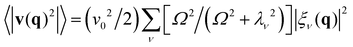 for disordered deterministic rotators.
In most experimental contexts, the extraction of the normal modes or their eigenvalues is unfeasible, except in specific scenarios like colloidal particle experiments.95–97 Current methods are often restricted to measuring in thermal equilibrium conditions and necessitate extensive data gathering. In the next subsection, we will therefore extend our findings to the framework of continuum elasticity theory, which only requires knowing the elastic constants of the material and is thus much easier to compute for real-world systems.
4.3 Continuum elastic formulation
To derive the continuum formulation, we begin by writing the equation of motion for the displacement vector field u(r) = r′(r) − r, which describes the deformed state r′(r) with respect to the equilibrium reference state r. As detailed in the ESI,† (ref. 92) in the presence of active forces this equation is given by![[u with combining dot above]](https://www.rsc.org/images/entities/b_char_0075_0307.gif) = ∇·σ + fact. = ∇·σ + fact. | (13) |
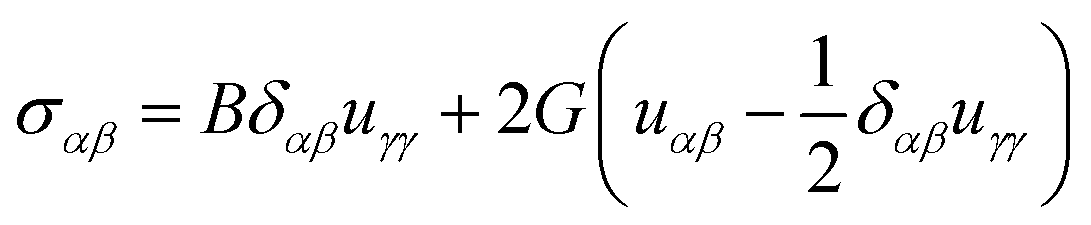 , and activity is introduced through self-propulsion forces defined by fact(r,t) = v0(r,t). In this expression for the stress tensor, B and G correspond respectively to the bulk and shear moduli of the isotropic solid, the strain tensor components
  are written in terms of spatial derivatives of the displacement vectors u(r) with respect to α,β ∈ {x,y}, and the summation over repeated indexes is assumed. We can see explicitly in eqn (13) that this active solid is distinct from odd active matter, which only considers internal active stresses that can be written in terms of effective moduli.58
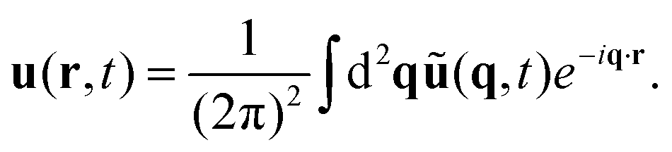
To proceed with the computations, we define the direct and inverse spatiotemporal Fourier transforms as

and write the continuum equation of motion (13) in Fourier space as

−iωũ(q,ω) = ![[f with combining tilde]](https://www.rsc.org/images/entities/b_char_0066_0303.gif) act(q,ω) − act(q,ω) − ![[Doublestruck D]](https://www.rsc.org/images/entities/char_e167.gif) (q)ũ(q,ω). (q)ũ(q,ω). | (14) |
(q) is a 2 × 2 dynamic matrix in Fourier space, given bywhere q2 = qx2 + qy2 (see ESI,† (ref. 92) for a detailed derivation), and we defined the active force fact(r,t) in Fourier space as

 | (15) |
We are interested in computing the velocity correlation functions. To do this, we begin by writing the orientational correlation in the continuum limit, replacing i(t) by a continuous field (r,t), with 〈i(t)·j(t′)〉 = δi,j〈(t)·(t′)〉. We then substitute the Kronecker delta δi,j by its Dirac counterpart, using δi,j → a2δ(r − r′), where a is the smallest characteristic length scale of the system, to obtain 〈(r,t)·(r′,t′)〉 = a2δ(r − r′)〈(t)·(t′)〉. From eqn (15), it is then clear that 〈act(q,ω)〉 = 0, and the second order correlation function C![[F with combining tilde]](https://www.rsc.org/images/entities/char_0046_0303.gif) = 〈act(q,ω)·act(q′,ω′)〉 is simply given by
= 〈act(q,ω)·act(q′,ω′)〉 is simply given by
 | (16) |
 , with Δq ≡ 2π/L. This also leads us to define the spatially discrete Fourier transform fact(q,ω) = act(q,ω)/a2 for discrete spatial wave vectors q but continuous frequency ω. The correlation function for this discrete Fourier transform, given by CF = 〈fact(q,ω)·fact(q′,ω′)〉, will be equal to
 | (17) |
![[q with combining circumflex]](https://www.rsc.org/images/entities/b_char_0071_0302.gif) + ũT(q,ω)⊥, with respect to the wave vector q, we can use ṽ(q,ω) = −iωũ(q,ω) to obtain the following expression for the mean-squared velocity in Fourier space
+ ũT(q,ω)⊥, with respect to the wave vector q, we can use ṽ(q,ω) = −iωũ(q,ω) to obtain the following expression for the mean-squared velocity in Fourier space | (18) |
 | (19) |
 .
.
Fig. 2(a) and (b) display how the longitudinal and transverse characteristic length scales described by eqn (19) change across the different regimes on the Dr − Ω plane. In Fig. 1(a), we used these equations to define the blue line as the Dr and Ω values for which the smallest characteristic length scale ξT is equal to the typical equilibrium distance between particles l0. Below this line, the system therefore develops mesoscopic scale correlations.
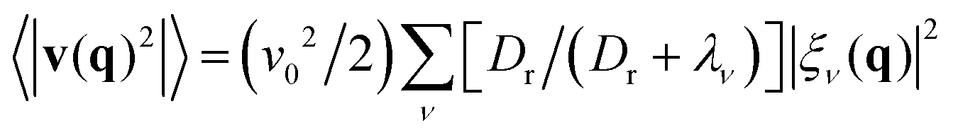
Next, we proceed to compute the mean-squared velocity 〈|v|2〉 of our system in real space. We can directly write the mean-squared velocity of all particles,  , in continuum form as
  , where 〈|v(q)|2〉 is given by eqn (18). The upper limit of this integral is set by the inverse particle size, i.e., by the maximum wave number qmax = 2π/a, where a is of the order of the particle size l0. Using
  , we can thus write
 | (20) |
Fig. 2(f) presents 〈|v|2〉/v02 as function of Dr for three different values of Ω = 1, 10, 20. The figure inset shows that 〈|v|2〉/v02 displays a minimum at intermediate noise strength Dr and high chirality (Ω = 10, 20). This implies that, as this minimum is reached, kinetic energy must be suppressed despite an increase in noise strength. Fig. 2(h) plots 〈|v|2〉/v02 as function of Ω for three different values of Dr = 1, 10, 20. In Fig. 1(a), we defined the magenta dashed line as the minimum of the normalized mean-squared velocity |〈v2〉|/v02, where most of the self-propulsion forces feed into the potential energy. This curve can be directly computed through a numerical integration of eqn (20).
Finally, we will now use the continuum formulation to investigate the collective temporal dynamics of the system (see ESI,† (ref. 92) Sections SIIIB-C for details). First, we directly calculate the velocity autocorrelation function as the integral over Fourier space
 | (21) |
 | (22) |
We finalize this section by exploring the scaling of the mean-squared velocity in eqn (18) in two limiting cases: the achiral active limit for χ = 1 (setting Ω = 0) and the limit with no noise χ = 0 (setting Dr = 0). In the achiral active case, 〈|v(q)|2〉 scales as ∼(ξTq)−2 and in the no noise case, it scales as 〈|v(q)|2〉 ∼ (ξTq)−4. In both limiting cases, 〈|v(q)|2〉 thus diverges for vanishing q, but with a different scaling.
In these two limiting cases, we can also compute the closed-form analytic mean-squared velocity. In the achiral active limit (Ω = 0), we get the previously obtained result93

which also shows the dominant scaling 〈|v|2〉 ∼ ξT−2 or 〈|v|2〉 ∼ ξL−2. Note that the mean-squared velocity will have small values in regimes of low chirality and low noise, which matches the regime where elastic energy is stored in the sheet, leading to the emergence of the mesoscopic correlated motion in the velocity fields.

5 Comparison with simulations
To compare the analytical predictions developed in the previous section with simulations, we computed the spatial velocity correlations in Fourier space 〈|v(q)|2〉 as well as the velocity and orientation autocorrelation functions (Cvv(t) = 〈v(t)·v(0)〉 and C(t) = 〈(t)·(0)〉, respectively) for a broad range of values of Dr and Ω. We focus on the two most salient regimes identified above: the emergence of correlated velocity fields for small Dr and Ω values (Section 5.1), and the extrema of the elastic and kinetic energy at high Dr and Ω values (Section 5.2).
5.1 Chiral mesoscopic range order
Fig. 3(a) presents simulation snapshots of the velocity angles showing the emergence of a CMRO state displaying correlated velocity fields for small values of Dr and Ω, as shown in the analytically computed state space diagram in Fig. 1(a).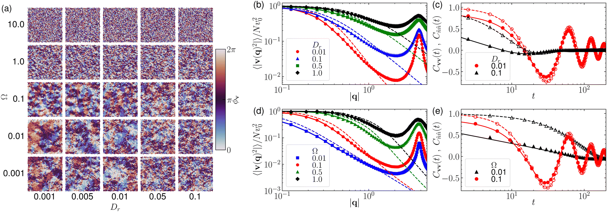 | ||
| Fig. 3 Emergence of chiral mesoscopic range order at low chirality and low noise. (a) Snapshots in the Ω − Dr parameter space illustrating the emergent spatial correlations on the particle velocity angles ϕv = tan−1(vy/vx). (b) and (d) Fourier space representation of the mean-squared velocity 〈|v(q)2|〉/Nv02 as a function of |q|, for different values of Dr with fixed Ω = 0.1, and for different values of Ω with fixed Dr = 0.01, respectively. Symbols represent simulations, solid lines result from the normal mode formulation in eqn (12), and dashed lines correspond to the continuum elastic approximation in eqn (18). (c) and (e) Normalized velocity autocorrelation functions Cvv(t) = 〈v(t)·v(0)〉/〈v(0)2〉 (filled symbols and solid lines) and orientation autocorrelation functions C(t) = 〈(t)·(0)〉 (open symbols and dashed lines) as a function of time t, for for different values of Dr and fixed Ω = 0.1, and for different values of Ω and fixed Dr = 0.01, respectively. Symbols represent simulations again, solid lines display the Cvv(t) in eqn (22), resulting from the continuum elastic formulation, and dashed lines correspond to the orientation autocorrelation in eqn (4). | ||
Fig. 3(b) and (d) present the spatial velocity correlations in Fourier space, 〈|v(q)2|〉 as a function of |q|, for a range of Dr = 0.01, 0.1, 0.5, 1.0 values with fixed Ω = 0.1, and for a range of Ω = 0.01, 0.1, 0.5, 1.0 values with fixed Dr = 0.01, respectively. We observe excellent agreement between the analytical normal mode formulation in eqn (12) and the simulation results (respectively solid lines and symbols), showing the emergence of correlated velocity fields for small Dr and Ω. The continuum elastic formulation in eqn (18), displayed as dashed lines, also shows good agreement with the simulations at low q, as expected.
Fig. 3(c) and (e), show the temporal autocorrelation functions for the orientations and normalized velocities, labeled C(t) and Cvv(t), respectively. Here, the C analytical curves in eqn (4) are represented by dashed lines and their numerical values by open symbols, while the Cvv analytical curves (22) are displayed as solid lines and their numerical values as solid symbols. In order to best match the numerical integration in eqn (22) to our simulations, we chose qmin and qmax as the smallest and largest simulated scales, as detailed in Appendix C. The red curves and symbols in Fig. 3(c) and (e) show that both autocorrelation functions, C and Cvv, display an oscillatory behavior for Dr = 0.01 and Ω = 0.1. The black curves and symbols show instead a non-oscillatory behavior for higher nose Dr = 0.1 in Fig. 3(c), and for lower chirality Ω = 0.01 in Fig. 3(e), presenting a faster decay in the Cvv case.
5.2 Elastic and kinetic energy extrema
We now compare our analytical and numerical results on the elastic and kinetic energy extrema found in the high noise Dr, high chirality Ω regime. First, we note that no such extrema is observed in active solids composed of achiral active particles, where the mean stored elastic energy always decreases with noise Dr. This also holds true for active solids composed of self-propelled particles with noisy chiral dynamics in the low chirality regime, with Ω < λmax, as it was shown in Fig. 1(a).In the high chirality regime Ω > λmax, however, there is a range of Dr values for which the mean potential energy stored in all modes increases with Dr, as shown in Fig. 2(e). This leads to a maximum in the mean stored elastic energy as a function of Dr, shown by the dashed green line in Fig. 1(a). In the same regime, the mean-squared velocity obtained from the continuum elastic formulation displays non-monotonic behavior, leading to the minimum in the kinetic energy shown in Fig. 2(f), which was displayed as the magenta dashed line in Fig. 1(a).
The non-monotonic features described above are also captured by the case of a single particle in a harmonic trap, which results in the curve with open black circles in Fig. 1(a). This can be seen in the mean square displacement 〈r2〉(t) presented in Fig. 4(a), the Cvv(t) in Fig. 4(b), and the 〈|v(q)|2〉 in Fig. 4(c), all in the high chirality regime (Ω = 10) and for noise strengths Dr = 1, 10, 100. We note that both the long-time 〈r2〉 values and the 〈|v(q)|2〉 curves exhibit non-monotonic behavior. However, the single particle Cvv result does not seem to capture this feature.
 | ||
| Fig. 4 Non-monotonic behavior (for high chirality and high noise) of chiral active solids as a function of noise Dr. (a) Mean-squared displacement 〈r2〉(t). The solid lines display analytical results recently obtained in ref. 89 for a single particle in a harmonic potential, given by eqn (28), as detailed in Appendix B. (b) Velocity and heading autocorrelation functions, Cvv(t) = 〈v(t)·v(0)〉/〈v(0)2〉 (filled symbols and solid lines) and C(t) = 〈(t)·(0)〉 (open symbols and dashed lines), as a function of time t. The solid lines result from the continuum elastic formulation in eqn (22) and the dashed lines correspond to plots of eqn (4). (c) Fourier space representation of 〈|v(q)2|〉/Nv02 as a function of |q|. The solid lines result from the normal mode formulation in eqn (12) and the dashed lines are obtained from the continuum elastic formulation in eqn (18). In all panels, the symbols represent simulations and we fixed v0 = 0.01 and Ω = 0.1. | ||
All these observations connect to the chiral glassy dynamics studied in ref. 89. In this work, the authors observe oscillatory temporal velocity autocorrelations and an emergent spatial correlation length in the limit of low Dr and low Ω, which we identify with the CMRO regime. They also find other states where the spatial correlations disappear but temporal correlations remain and a state without spatial or temporal correlations, corresponding to the CD and DD regimes, respectively. In the same study,89 the authors discovered what they refer to as a ‘hammering state’, where particles oscillate in their potential cages, with a maximum in the mean-squared displacement (MSD) with respect to the diffusion constant. We can now identify this state with the maximum of the potential energy with respect to Dr, in the CD regime, as described analytically by our results.
6 Analysis of melting behavior at high activity
The solid to liquid transition in systems of active particles has been extensively studied, starting with the observation that, in the high density and low motility limit, active Brownian particles form crystals99 if they are monodisperse and glasses otherwise.100In a two-dimensional equilibrium crystal, the melting transition is a multifaceted process, characterized by the progressive disintegration of, both, positional and orientational coherence. In systems characterized by short-range interactions, melting manifests either as a first-order solid–liquid transition or via the sequential two-phase KTHNY mechanism involving solid–hexatic and hexatic–liquid transitions.55,101–103 Unlike passive systems, active crystals can autonomously organize and transition into an active fluid state facilitated by self-propulsion and the interaction forces. In particular, however, the melting transition in active particle models of biological tissues occurs through a continuous solid–hexatic transition that is then followed by a continuous hexatic–liquid transition.104,105
The glass transition has been intensively studied in the context of active Brownian particles without chirality.66,72,82,85,106 These efforts have shown that its differences with the usual thermal glass transition can be subtle, and that it is governed by an effective temperature Teff = v02/2Dr. This result only changes in the limit Dr → 0,107 where the coherent mesoscopic length scale becomes large93,108 and starts influencing the transition properties.86,106,109 On the other hand, glasses of chiral active particles have only been studied in detail up to now in ref. 89, and we discussed how this work connects to our results in the previous section.
We find in our simulation that, in the high activity limit, a solid triangular monocrystaline structure of chiral active particles will eventually melt. Since a detailed description of this transition would be beyond the scope of this work, we will focus instead on testing the tolerance of our analytic predictions to an increasing level of activity. Fig. 5 plots the numerical values of three different predicted quantities for increasing active speed v0 levels. We consider fixed noise and chirality values that place the system in the CMRO regime, incrementally increasing v0 to observe the melting behavior. The MSD exhibits trapped oscillatory behavior up to v0 = 0.12, where melting begins, as shown in Fig. 5(a). The velocity autocorrelation functions in Fig. 5(b) and spatial velocity correlation functions in Fig. 5(c) also show that the deviation from the theory starts at v0 ≳ 0.1. We include the corresponding dynamics of the velocity fields in the CMRO regime, with Dr = 0.01 and Ω = 0.1, in the ESI,† (ref. 92) setting v0 = 0.1 for Movie S6 and v0 = 0.12 for Movie S7. These results clearly indicate that our analytic methods remain in excellent agreement with simulations until just below the melting transition, and that they start deviating at high activity. Nonetheless, we note that both the temporal oscillations and the mesoscale correlations persist, albeit with modified scaling. The latter is in agreement with what has been observed when fitting non-chiral models to cell sheet data93 and in simulations of active Brownian particles (ABPs) at higher activity levels.93,109 This also explains why our results can remain predictive for the active glassy dynamics investigated in ref. 89.
 | ||
| Fig. 5 Melting behavior of chiral active solids. The symbols result from simulations with different self-propulsion speed v0 values, for Dr = 0.01 and Ω = 0.1. (a) Mean-squared displacement 〈r2〉(t) as function of time t. (b) Velocity autocorrelation Cvv(t) = 〈v(t)·v(0)〉/〈v(0)2〉 as a function of time t. The solid line is obtained from the continuum elastic formulation in eqn (22). (c) Fourier space representation of 〈|v(q)2|〉/Nv02 as a function of |q|. The solid line results from the normal mode formulation in eqn (12) and the dashed line, from the continuum elastic formulation in eqn (18). | ||
7 Extension to heterogeneous systems
We now extend our results to heterogeneous systems where the active particles can have different dynamical properties. We will first study binary mixtures of disks with different chirality and rotational diffusion coefficients in Section 7.1, and then cases where the disks have a distribution of chirality and diffusion values in Section 7.2.7.1 Binary mixtures
We consider an active solid composed of two particle species, A and B, differentiated by their Dr and Ω values, and with corresponding packing fractions, ϕA and ϕB. Since the active driving produces time-correlated but spatially independent noise, as shown by eqn (7) and (16), the total driving noise from two species can be computed as a simple superposition, with no particle-particle cross-correlations. Then, quantities such as 〈|v(q)|2〉 and 〈v(t)·v(0)〉, which we analytically derived in Section 4, can be expressed as the mean of their A and B contributions, weighted by their respective fractions. In the linear response regime, the general expression for f = |v(q)|2 or for f = v(t)·v(0) is therefore given by | (23) |
To illustrate the effects of having binary mixtures of particles, we present simulations and analytical results for three different species combinations, all displaying chiral mesoscopic range order, in the CMRO regime. Fig. 6(a) and (b) respectively show the Cvv(t) and 〈|v(q)|2〉/Nv02 curves obtained for three different binary mixtures with equal fractions (ϕA/ϕB = 1) and total packing fraction ϕ = 1. First, the (i) curves show the single species case, as a reference. Second, the (ii) curves correspond to mixtures of achiral (ΩA = 0) and chiral (ΩB = 0.1) active particles with equal rotational diffusion coefficients DAr = DBr = 0.01. Third, the (iii) curves present mixtures of particles with two different chirality values, ΩA = 0.1 and ΩB = 0.2, and the same DAr = DBr = 0.01 (see also Movie S9 in the ESI,† (ref. 92)). Finally, the (iv) curves display mixtures of particles with equal chirality values ΩA = ΩB = 0.1 and two different rotational diffusion coefficients, DAr = 0.01 and DBr = 0.1.
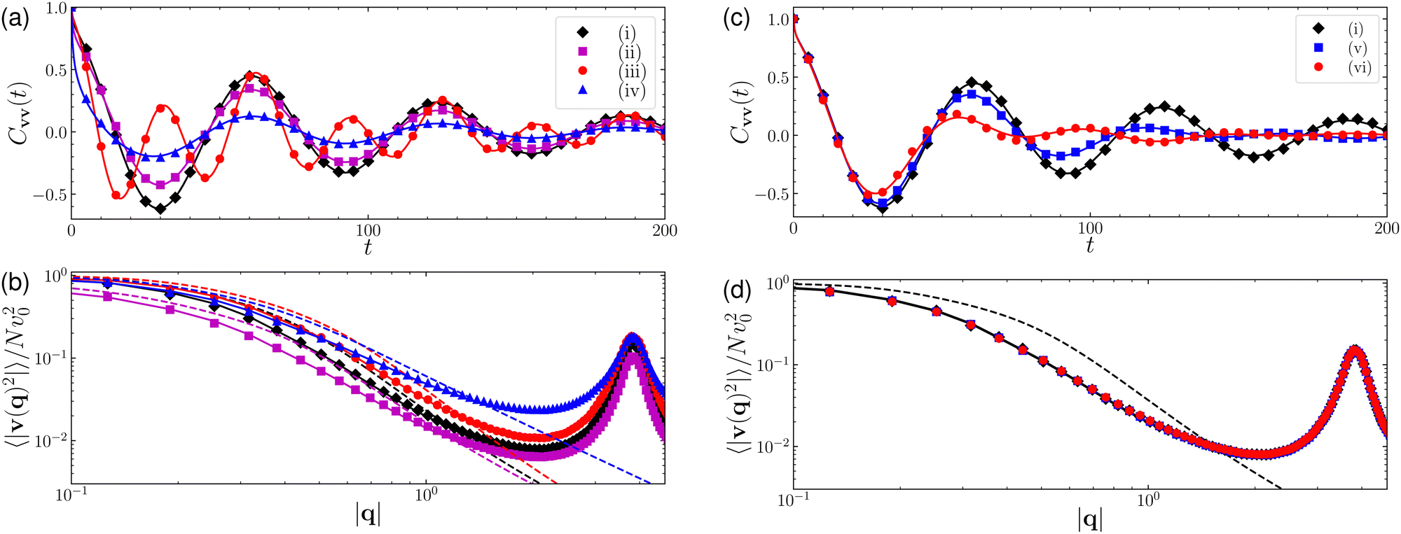 | ||
| Fig. 6 Effects of heterogeneity in chiral active solids. (a) and (b) Binary mixtures of species A and B with packing fractions ϕA = ϕB = 1/2 for: (i) DAr = DBr = 0.01 and ΩA = ΩB = 0.1 (homogeneous case); (ii) DAr = DBr = 0.01, ΩA = 0.0, and ΩB = 0.1; (iii) DAr = DBr = 0.01, ΩA = 0.1, and ΩB = 0.2; and (iv) DAr = 0.01, DBr = 0.1, and ΩA = ΩB = 0.1. (c) and (d) Heterogeneous mixtures of particles with uniform distributions of (Dr,Ω) values spanning (v) ±20% and (vi) ±40% of their means, and homogeneous case (i) for comparison. In all panels, symbols represent numerical simulations. In panels (a) and (c), the solid lines plot the velocity autocorrelation Cvv(t) obtained from the continuum elastic formulation. In panels (b) and (d), the dashed and solid lines correspond to the mean-squared velocity 〈|v(q)|2〉/Nv02 resulting respectively from the continuum elastic formulation and the normal mode formulation. | ||
In Fig. 6(a) we can see that the clear oscillations in the velocity autocorrelation are suppressed when we consider achiral–chiral mixtures (ii), compared to the single species case (i). We can also see that, in systems with two different chirality values (iii), the velocity autocorrelation function displays oscillations with the two corresponding periods, 2π/ΩA and 2π/ΩB. Finally, the figure shows that mixtures of chiral active particles with two different rotational diffusion coefficients (iv) suppress this oscillatory behavior and follow the lower persistence length of the population with the highest Dr. In Fig. 6(b) we can see that binary mixtures of achiral and chiral active particles (ii) enhance the ordering in the CMRO state when compared to the homogeneous case (i), decaying at lower |q| values. On the other hand, we see that chiral active binary mixtures with, both, different chirality values (iii) and different rotational diffusion coefficients (iv) suppress the ordering in the CMRO state when compared to the homogeneous case (i), decaying at larger |q| values. In addition, we note that the analytic superposition results (solid and dashed lines) show an excellent agreement with the simulation results (symbols) for all curves in Fig. 6(a) and (b), thus validating eqn (23).
Finally, Fig. S4 in the ESI,† (ref. 92) further illustrates how oscillations appear, disappear, and interfere by presenting the velocity time correlations obtained from eqn (23) for a range of binary mixtures.
7.2 Heterogeneous particles
We now further extend our analyses to investigate active solids composed of heterogeneous particles with a distribution of dynamical properties. To do this, we consider a complex random mixture of n different types of active particles, each with corresponding packing fraction ϕ1,ϕ2,…,ϕn, adding up to a total packing fraction . We can then obtain a general expression for the combined values of f = |v(q)|2 or f = v(t)·v(0) in terms of the individual components as
 | (24) |
Fig. 6(c) and (d) present the analytical and simulated spatiotemporal correlation functions of the active solid dynamics of a set of particles with a uniformly distributed range of Dr and Ω values, spanning: (i) ±0%, (v) ±20%, and (vi) ±40% with respect to their mean 〈(Dr,Ω)〉 = (0.01,0.1). We can see in Fig. 6(c) a clear deviation of the velocity–velocity correlations Cvv in the heterogeneous cases, (v) and (vi), with respect to the homogeneous case (i). We note that the analytical superposition of eqn (22) using eqn (24), displayed as solid lines, perfectly captures the simulation results, represented by symbols. In Fig. 6(d), we see that 〈|v(q)|2〉/Nv02 is practically invariant under changes in the Dr and Ω parameters. We also note that the analytical superposition of eqn (12) and (18), represented respectively by a solid and a dashed line, can properly capture our simulation results. The figure shows that the spatial velocity correlations are insensitive to the heterogeneity of the system, but that the temporal velocity autocorrelation is affected by it. Indeed, increased heterogeneity in particle chirality leads to a desynchronization of the oscillations, while increased heterogeneity in Dr does not (as shown in Fig. S5a and c in the ESI,† (ref. 92)). The spatial correlations are not affected in either case (see Fig. S5b and d in the ESI,† (ref. 92)). We can thus predict that the oscillatory dynamics will only be apparent in systems of active particles with relatively homogeneous levels of chirality.
8 Conclusions
In this work, we formulated the analytic linear response theory for an active solid composed of self-propelled particles with noisy chiral dynamics. We considered a minimal model with the potential for describing a broad range of systems, ranging from artificial active solids made of chiral self-propelled robots to biological tissues with emergent macroscopic chiral order. We developed an analytic formulation that allowed us to fully describe all the observed dynamics in the linear regime, perfectly matching our numerical results.We described the emergence of four different types of dynamics in the phase space described by the chirality Ω and the rotational diffusion coefficient Dr. For small enough Dr and Ω, we observe chiral (CMRO) and achiral (MRO) self-organized states displaying mesoscopic range order. For larger Dr and Ω, we only find chiral (CD) and achiral (DD) disordered states. In all cases, the chiral sates appear for Dr < Ω and the achiral states, for Dr > Ω. We then explored the dynamics of the melting regime by increasing the activity v0, showing that our analytic results for the spatial velocity correlations and the temporal velocity autocorrelations agree with simulations up to an active speed v0 ≈ 0.1, just below v0 = 0.12, the melting point obtained using our active solid theory. Finally, we showed that our analytic approaches can be extended to consider particles with heterogeneous dynamical features, including different chirality and rotational diffusion levels. We derived analytic superposition expressions for binary and more complex mixtures of heterogeneous active particles, demonstrating their excellent agreement with simulations.
Our work is consistent with the (relatively sparse) literature on chiral ABP solids. Notably we recover the oscillatory correlations and ‘hammering’ resonance observed by Debets et al.89 in the glassy state. In addition, our work also seems to be consistent with recent results obtained by Caprini et al.90 while exploring the emergence of self-reverting vortices in the absence of alignment forces, as a result of the interplay between attractive interactions and chirality. They found two kinds of vortices, with either persistent or oscillatory behavior, which could correspond to our observation that the correlated velocity fields in the mesoscopic range can either be persistent (MRO) or oscillatory (CMRO). However, due to subtle differences in the equations (that include inertia and spatial noise in their case), we cannot currently compare our results quantitatively.
There are various possible extensions to our framework. We could, for example, introduce hydrodynamic interactions, which would modify our findings. It is indeed relatively straightforward to add a mobility matrix to the spatial equation, e.g. through a pair dissipation term λ(vi − vj), where λ is the ratio of pair to single particle friction. This leads to yet another modified mesoscopic length scale that is basically the hydrodynamic length scale  . However, wet hydrodynamic interactions also introduce torque couplings between particles, which invalidates our linear response approach, as the angular equation cannot be solved independently anymore. Although this will likely lead to very interesting collective phenomenology, similar to that in ref. 50 and 51, such analysis is still beyond our reach.
We hope that the general analytical description of dense, solid chiral dry active systems in this paper can help establish the foundations for a systematic understanding of the emergent dynamics in this type of systems. Future research could explore the scalability of our theory, its practical applications in synthetic biology, and its potential impact on the design and control of rotating correlated velocity fields in natural or artificial active solids.
Author contributions
Conceptualization: Amir Shee, Silke Henkes, and Cristián Huepe; analytic calculations and numerical simulations: Amir Shee; writing – original draft preparation: Amir Shee; writing – review and editing: Amir Shee, Silke Henkes, and Cristián Huepe; supervision: Silke Henkes and Cristián Huepe.Data availability
The data supporting this article have been included as part of the ESI.† All relevant datasets have been archived and can be provided for replication and further research purposes.Conflicts of interest
There are no conflicts to declare.Appendices
A. Orientation autocorrelation
We adopt the method for the exact moments calculation of stiff chains described in Hermans et al.110 to determine the moments for the active dynamics case. This approach, previously applied in,111–113 is used to obtain the exact dynamics for a chiral active Brownian particle in a harmonic trap, as detailed in Debets et al.89 Utilizing the Laplace transform in eqn (3) while defining the mean of an observable as
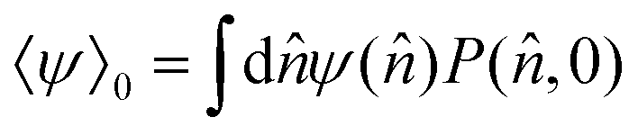
  , multiplying by ψ(), and integrating over all possible , we find
| −〈ψ〉0 + s〈ψ〉s = Dr〈∇2ψ〉s + Ω〈⊥·∇ψ〉s. | (25) |
 . Without loss of generality, we can define the initial condition as following P(,0) = δ( − 0), where 0 is the initial orientation of the particle.
Using eqn (25), we compute the orientational correlation as a function of time. We set the initial particle headings as satisfying 〈〉 = 0. To compute 〈〉, we then use ψ = in eqn (25) to obtain
 | (26) |
⊥〉s, starting from an initial perpendicular orientation 〈⊥〉 = ⊥0, by using ψ = ⊥ in eqn (25), which gives 〈⊥〉s = (⊥0 − Ω〈〉s)/(s + Dr). Substituting back into eqn (26) produces | (27) |
(t)〉 = e−Drt[0cos(Ωt) + ⊥0sin(Ωt)]. Finally, by computing the dot product with the initial heading, we find the orientation autocorrelation expression in eqn (4).
B. Single chiral active Brownian particle in a harmonic trap
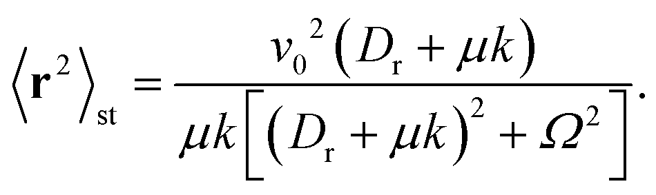
Following procedure similar to that used in the orientation autocorrelation calculation, we can compute the MSD of a single chiral active Brownian particle in a harmonic trap, as previously done in ref. 89, finding | (28) |
 | (29) |
 | (30) |
 line, shown as the black dotted line on the Dr − Ω plane in Fig. 1(a), for μ = 1 and k = 1. This suggests that the reentrant transition with increasing Dr (from low 〈r2〉st to high 〈r2〉st, with maximum at
  , and then back to low 〈r2〉st) occurs only when chirality is high, that is, for Ω > μk.
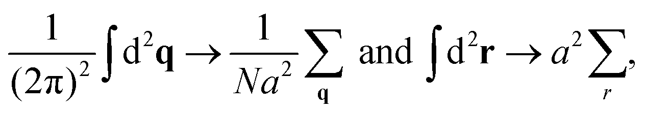
C. Determining the elastic moduli and continuum theory to compare with simulations
To determine the elastic moduli, we first equilibrate the steady state configurations by letting v0 = 0 in eqn (1). The disks reach their equilibrium positions after a long integration time. Using these positions, we then construct a dynamical Hessian matrix. We transform this matrix to Fourier space with appropriate grid space q. The resulting longitudinal and transverse eigenvalues thus correspond to (B + G)q2 and Gq2, respectively. We then determine the bulk modulus B and shear modulus G by performing a linear fit of the radially averaged longitudinal and transverse eigenvalues against q2, focusing on the limit with q2 ≤ 1. Our calculations for soft disks thus yield the following values for the moduli: : G = 0.61, B = 2.03, and (B + G)/G = 4.33, with relative error lower than 1% (averaging over 10 independent estimations).When comparing our numerical results to the continuum theory, simulations are carried out for relatively large but finite systems of size L, with minimum length scale given by the particle size a = 2r0, where r0 is the particle radius. Our numerical analysis is therefore performed using discrete Fourier transforms, in a finite grid, whereas our analytical calculations are carried out in the continuum limit, by setting L → ∞ and a → 0.
Finally, to achieve consistency between the discrete and continuum approaches, we use the following continuous Fourier transform
 | (31) |
where N = 4ϕL2/πa2 and ϕ is the packing fraction of the system (close to 1 for dense systems). In the sum, q takes discrete values defined by the geometry of the system. For instance, for a square lattice of linear size L, q ≡ (qx,qy) = 2π/L(m,n), with integers m, n satisfying 0 ≤ m,n ≤ L/a − 1. Thus, the discrete space Fourier transform u(q,t) is related to the continuous Fourier transform ũ(q,t) viaũ(q,t) = a2u(q,t).
Acknowledgements
This project was made possible through the support of Grant 62213 from the John Templeton Foundation. SH would like to acknowledge support of the NWO through her Leiden University startup package within the sector plan.Notes and references
- F. Kümmel, B. ten Hagen, R. Wittkowski, I. Buttinoni, R. Eichhorn, G. Volpe, H. Löwen and C. Bechinger, Phys. Rev. Lett., 2013, 110, 198302 CrossRef.
- C. Bechinger, R. Di Leonardo, H. Löwen, C. Reichhardt, G. Volpe and G. Volpe, Rev. Mod. Phys., 2016, 88, 45006 CrossRef.
- T. Mano, J. B. Delfau, J. Iwasawa and M. Sano, Proc. Natl. Acad. Sci. U. S. A., 2017, 114, E2580–E2589 CrossRef.
- B. Zhang and A. Snezhko, Phys. Rev. Lett., 2022, 128, 218002 CrossRef PubMed.
- B. A. Grzybowski, H. A. Stone and G. M. Whitesides, Nature, 2000, 405(6790), 1033–1036 CrossRef PubMed.
- J.-M. Cruz, O. Díaz-Hernández, A. Castañeda-Jonapá, G. Morales-Padrón, A. Estudillo and R. Salgado-García, Soft Matter, 2024, 20, 1199–1209 RSC.
- H. S. Jennings, Am. Nat., 1901, 35, 369–378 CrossRef.
- M. Loose and T. J. Mitchison, Nat. Cell Biol., 2014, 16, 38–46 CrossRef CAS PubMed.
- Y. Sumino, K. H. Nagai, Y. Shitaka, D. Tanaka, K. Yoshikawa, H. Chaté and K. Oiwa, Nature, 2012, 483, 448–452 CrossRef CAS.
- C. J. Brokaw, D. J. Luck and B. Huang, J. Cell Biol., 1982, 92, 722–732 CrossRef CAS.
- W. R. DiLuzio, L. Turner, M. Mayer, P. Garstecki, D. B. Weibel, H. C. Berg and G. M. Whitesides, Nature, 2005, 435, 1271–1274 CrossRef CAS.
- E. Lauga, W. R. DiLuzio, G. M. Whitesides and H. A. Stone, Biophys. J., 2006, 90, 400–412 CrossRef CAS.
- I. H. Riedel, K. Kruse and J. Howard, Science, 2005, 309, 300–303 CrossRef.
- R. Nosrati, A. Driouchi, C. M. Yip and D. Sinton, Nat. Commun., 2015, 6, 8703 CrossRef PubMed.
- S. van Teeffelen and H. Löwen, Phys. Rev. E: Stat., Nonlinear, Soft Matter Phys., 2008, 78, 020101 CrossRef.
- S. Van Teeffelen, U. Zimmermann and H. Löwen, Soft Matter, 2009, 5, 4510–4519 RSC.
- M. Mijalkov and G. Volpe, Soft Matter, 2013, 9, 6376–6381 RSC.
- G. Volpe, S. Gigan and G. Volpe, Am. J. Phys., 2014, 82, 659–664 CrossRef.
- H. Löwen, Eur. Phys. J.: Spec. Top., 2016, 225, 2319–2331 Search PubMed.
- F. J. Sevilla, Phys. Rev. E, 2016, 94, 062120 CrossRef.
- T. Markovich, E. Tjhung and M. E. Cates, New J. Phys., 2019, 21, 112001 CrossRef CAS.
- O. Chepizhko and T. Franosch, New J. Phys., 2020, 22, 073022 CrossRef.
- L. Caprini, H. Löwen and U. Marini Bettolo Marconi, Soft Matter, 2023, 19, 6234–6246 RSC.
- R. Di Leonardo, D. Dell’Arciprete, L. Angelani and V. Iebba, Phys. Rev. Lett., 2011, 106, 038101 CrossRef CAS.
- G. Araujo, W. Chen, S. Mani and J. X. Tang, Biophys. J., 2019, 117, 346–354 CrossRef CAS PubMed.
- M. Böhmer, Q. Van, I. Weyand, V. Hagen, M. Beyermann, M. Matsumoto, M. Hoshi, E. Hildebrand and U. B. Kaupp, EMBO J., 2005, 24, 2741–2752 CrossRef PubMed.
- J. Taktikos, V. Zaburdaev and H. Stark, Phys. Rev. E: Stat., Nonlinear, Soft Matter Phys., 2011, 84, 41924 CrossRef.
- J. G. Gibbs and Y. Zhao, Small, 2009, 5, 2304–2308 CrossRef CAS.
- J. G. Gibbs, S. Kothari, D. Saintillan and Y.-P. Zhao, Nano Lett., 2011, 11, 2543–2550 CrossRef CAS PubMed.
- J. Denk, L. Huber, E. Reithmann and E. Frey, Phys. Rev. Lett., 2016, 116, 178301 CrossRef.
- M. Bär, R. Großmann, S. Heidenreich and F. Peruani, Annu. Rev. Condens. Matter Phys., 2020, 11, 441–466 CrossRef.
- B. Zhang, A. Sokolov and A. Snezhko, Nat. Commun., 2020, 11, 4401 CrossRef CAS PubMed.
- A. I. Campbell, R. Wittkowski, B. Ten Hagen, H. Löwen and S. J. Ebbens, J. Chem. Phys., 2017, 147, 84905 CrossRef.
- R. J. Archer, A. I. Campbell and S. J. Ebbens, Soft Matter, 2015, 11, 6872–6880 RSC.
- T. Lei, C. Zhao, R. Yan and N. Zhao, Soft Matter, 2023, 19, 1312–1329 RSC.
- B. Liebchen and D. Levis, Phys. Rev. Lett., 2017, 119, 058002 CrossRef.
- D. Levis and B. Liebchen, J. Phys.: Condens. Matter, 2018, 30, 084001 CrossRef PubMed.
- G. J. Liao and S. H. Klapp, Soft Matter, 2018, 14, 7873–7882 RSC.
- A. Kaiser and H. Löwen, Phys. Rev. E: Stat., Nonlinear, Soft Matter Phys., 2013, 87, 032712 CrossRef.
- Y. Liu, Y. Yang, B. Li and X.-Q. Feng, Soft Matter, 2019, 15, 2999–3007 RSC.
- Z. Ma and R. Ni, J. Chem. Phys., 2022, 156, 21102 CrossRef CAS.
- V. Semwal, J. Joshi and S. Mishra, Phys. A, 2024, 634, 129435 CrossRef.
- J. Bickmann, S. Bröker, J. Jeggle and R. Wittkowski, J. Chem. Phys., 2022, 156, 194904 CrossRef CAS PubMed.
- Q.-L. Lei and R. Ni, Proc. Natl. Acad. Sci. U. S. A., 2019, 116, 22983–22989 CrossRef CAS PubMed.
- Q.-L. Lei, M. P. Ciamarra and R. Ni, Sci. Adv., 2019, 5, eaau7423 CrossRef PubMed.
- B. Hrishikesh and E. Mani, Soft Matter, 2023, 19, 225–232 RSC.
- D. Levis and B. Liebchen, Phys. Rev. E, 2019, 100, 012406 CrossRef CAS.
- B.-Q. Ai, S. Quan and F. G. Li, New J. Phys., 2023, 25, 063025 CrossRef.
- S. Ceron, K. O’Keeffe and K. Petersen, Nat. Commun., 2023, 14, 940 CrossRef CAS PubMed.
- E. S. Bililign, F. Balboa Usabiaga, Y. A. Ganan, A. Poncet, V. Soni, S. Magkiriadou, M. J. Shelley, D. Bartolo and W. T. Irvine, Nat. Phys., 2022, 18, 212–218 Search PubMed.
- T. H. Tan, A. Mietke, J. Li, Y. Chen, H. Higinbotham, P. J. Foster, S. Gokhale, J. Dunkel and N. Fakhri, Nature, 2022, 607, 287–293 CrossRef CAS.
- K. Drescher, K. C. Leptos, I. Tuval, T. Ishikawa, T. J. Pedley and R. E. Goldstein, Phys. Rev. Lett., 2009, 102, 168101 CrossRef PubMed.
- A. P. Petroff, X.-L. Wu and A. Libchaber, Phys. Rev. Lett., 2015, 114, 158102 CrossRef.
- J. Yan, S. C. Bae and S. Granick, Soft Matter, 2015, 11, 147–153 RSC.
- Z.-F. Huang, A. M. Menzel and H. Löwen, Phys. Rev. Lett., 2020, 125, 218002 CrossRef CAS.
- T. Ishikawa, T. J. Pedley, K. Drescher and R. E. Goldstein, J. Fluid Mech., 2020, 903, A11 CrossRef.
- A. P. Petroff, C. Whittington and A. Kudrolli, Phys. Rev. E, 2023, 108, 014609 Search PubMed.
- M. Fruchart, C. Scheibner and V. Vitelli, Annu. Rev. Condens. Matter Phys., 2023, 14, 471–510 Search PubMed.
- S. Henkes, Y. Fily and M. C. Marchetti, Phys. Rev. E: Stat., Nonlinear, Soft Matter Phys., 2011, 84, 040301 Search PubMed.
- G. Lin, Z. Han and C. Huepe, New J. Phys., 2021, 23, 023019 Search PubMed.
- P. Baconnier, D. Shohat, C. H. López, C. Coulais, V. Démery, G. Düring and O. Dauchot, Nat. Phys., 2022, 18, 1234–1239 Search PubMed.
- G. Lin, Z. Han, A. Shee and C. Huepe, Phys. Rev. Lett., 2023, 131, 168301 CrossRef PubMed.
- P. Baconnier, D. Shohat and O. Dauchot, Phys. Rev. Lett., 2023, 130, 028201 CrossRef PubMed.
- H. Xu, Y. Huang, R. Zhang and Y. Wu, Nat. Phys., 2023, 19, 46–51 Search PubMed.
- L. Berthier and J. Kurchan, Nat. Phys., 2013, 9, 310–314 Search PubMed.
- L. Berthier, Phys. Rev. Lett., 2014, 112, 220602 CrossRef.
- G. Szamel, E. Flenner and L. Berthier, Phys. Rev. E: Stat., Nonlinear, Soft Matter Phys., 2015, 91, 062304 CrossRef PubMed.
- V. E. Debets and L. M. C. Janssen, J. Chem. Phys., 2023, 159, 14502 CrossRef CAS.
- R. Ni, M. A. C. Stuart and M. Dijkstra, Nat. Commun., 2013, 4, 2704 CrossRef.
- D. Bi, X. Yang, M. C. Marchetti and M. L. Manning, Phys. Rev. X, 2016, 6, 021011 Search PubMed.
- A. Liluashvili, J. Ónody and T. Voigtmann, Phys. Rev. E, 2017, 96, 062608 CrossRef PubMed.
- S. K. Nandi, R. Mandal, P. J. Bhuyan, C. Dasgupta, M. Rao and N. S. Gov, Proc. Natl. Acad. Sci. U. S. A., 2018, 115, 7688–7693 CrossRef.
- G. Szamel, J. Chem. Phys., 2019, 150, 124901 CrossRef PubMed.
- R. Mandal and P. Sollich, Phys. Rev. Lett., 2020, 125, 218001 CrossRef PubMed.
- J. Reichert, S. Mandal and T. Voigtmann, Phys. Rev. E, 2021, 104, 044608 CrossRef.
- J. Reichert and T. Voigtmann, Soft Matter, 2021, 17, 10492–10504 RSC.
- J. Reichert, L. F. Granz and T. Voigtmann, Eur. Phys. J. E: Soft Matter Biol. Phys., 2021, 44, 27 CrossRef.
- V. E. Debets, X. M. de Wit and L. M. Janssen, Phys. Rev. Lett., 2021, 127, 278002 CrossRef CAS.
- V. E. Debets and L. M. C. Janssen, Phys. Rev. Res., 2022, 4, L042033 CrossRef CAS.
- G. Janzen and L. M. C. Janssen, Phys. Rev. Res., 2022, 4, L012038 CrossRef CAS.
- M. Paoluzzi, D. Levis and I. Pagonabarraga, Commun. Phys., 2022, 5, 111 CrossRef.
- E. Flenner, G. Szamel and L. Berthier, Soft Matter, 2016, 12, 7136–7149 RSC.
- G. Szamel, Phys. Rev. E, 2016, 93, 012603 CrossRef.
- M. Feng and Z. Hou, Soft Matter, 2017, 13, 4464–4481 RSC.
- L. Berthier, E. Flenner and G. Szamel, New J. Phys., 2017, 19, 125006 CrossRef.
- E. Flenner and G. Szamel, Phys. Rev. E, 2020, 102, 022607 CrossRef PubMed.
- L. Caprini and U. Marini Bettolo Marconi, Soft Matter, 2021, 17, 4109–4121 RSC.
- G. Szamel and E. Flenner, Europhys. Lett., 2021, 133, 60002 CrossRef.
- V. E. Debets, H. Löwen and L. M. Janssen, Phys. Rev. Lett., 2023, 130, 058201 CrossRef CAS.
- L. Caprini, B. Liebchen and H. Löwen, Commun. Phys., 2024, 7, 153 CrossRef.
- Y. Kuroda, T. Kawasaki and K. Miyazaki, arXiv, 2024, preprint, arXiv:2402.19192 DOI:10.48550/arXiv.2402.19192.
- See ESI† at https://doi.org/10.1039/D4SM00958D for description of simulation movies, analytic calculations, which include ref. 93 and 114.
- S. Henkes, K. Kostanjevec, J. M. Collinson, R. Sknepnek and E. Bertin, Nat. Commun., 2020, 11, 1405 CrossRef CAS.
- L. Caprini and U. Marini Bettolo Marconi, Soft Matter, 2019, 15, 2627–2637 RSC.
- K. Chen, W. G. Ellenbroek, Z. Zhang, D. T. Chen, P. J. Yunker, S. Henkes, C. Brito, O. Dauchot, W. Van Saarloos, A. J. Liu and A. G. Yodh, Phys. Rev. Lett., 2010, 105, 025501 CrossRef PubMed.
- S. Henkes, C. Brito and O. Dauchot, Soft Matter, 2012, 8, 6092 RSC.
- J. Melio, S. E. Henkes and D. J. Kraft, Phys. Rev. Lett., 2024, 132, 078202 CrossRef CAS.
- S. Garcia, E. Hannezo, J. Elgeti, J.-F. Joanny, P. Silberzan and N. S. Gov, Proc. Natl. Acad. Sci. U. S. A., 2015, 112, 15314–15319 CrossRef CAS PubMed.
- J. Bialké, T. Speck and H. Löwen, Phys. Rev. Lett., 2012, 108, 168301 CrossRef.
- Y. Fily, S. Henkes and M. C. Marchetti, Soft Matter, 2014, 10, 2132–2140 RSC.
- J. G. Dash, Rev. Mod. Phys., 1999, 71, 1737–1743 CrossRef CAS.
- U. Gasser, J. Phys.: Condens. Matter, 2009, 21, 203101 CrossRef CAS.
- Y.-W. Li and M. P. Ciamarra, Phys. Rev. Lett., 2020, 124, 218002 CrossRef CAS.
- P. Digregorio, D. Levis, A. Suma, L. F. Cugliandolo, G. Gonnella and I. Pagonabarraga, Phys. Rev. Lett., 2018, 121, 098003 CrossRef CAS.
- A. Pasupalak, L. Yan-Wei, R. Ni and M. Pica Ciamarra, Soft Matter, 2020, 16, 3914–3920 RSC.
- L. Berthier, E. Flenner and G. Szamel, J. Chem. Phys., 2019, 150, 200901 CrossRef.
- R. Mandal, P. J. Bhuyan, P. Chaudhuri, C. Dasgupta and M. Rao, Nat. Commun., 2020, 11, 2581 CrossRef CAS.
- L. Caprini, U. M. B. Marconi, C. Maggi, M. Paoluzzi and A. Puglisi, Phys. Rev. Res., 2020, 2, 023321 CrossRef CAS.
- Y.-E. Keta, J. U. Klamser, R. L. Jack and L. Berthier, Phys. Rev. Lett., 2024, 132, 218301 CrossRef PubMed.
- J. Hermans and R. Ullman, Physica, 1952, 18, 951–971 CrossRef.
- A. Shee, A. Dhar and D. Chaudhuri, Soft Matter, 2020, 16, 4776–4787 RSC.
- D. Chaudhuri and A. Dhar, J. Stat. Mech.: Theory Exp., 2021, 2021, 013207 CrossRef.
- A. Shee and D. Chaudhuri, J. Stat. Mech.: Theory Exp., 2022, 2022, 013201 CrossRef.
- P. M. Chaikin and T. C. Lubensky, Principles of Condensed Matter Physics, Cambridge University Press, Cambridge, 1995 Search PubMed.
Footnote |
| † Electronic supplementary information (ESI) available. See DOI: https://doi.org/10.1039/d4sm00958d |
| This journal is © The Royal Society of Chemistry 2024 |