DOI:
10.1039/D4SM00634H
(Paper)
Soft Matter, 2024,
20, 8395-8406
Controlling wall–particle interactions with activity
Received
24th May 2024
, Accepted 20th September 2024
First published on 30th September 2024
Abstract
We theoretically determine the effective forces on hard disks near walls embedded inside active nematic liquid crystals. When the disks are sufficiently close to the wall and the flows are sufficiently slow, we can obtain exact expressions for the effective forces. We find these forces and the dynamics of disks near the wall depend both on the properties of the active nematic and on the anchoring conditions on the disks and the wall. Our results show that the presence of active stresses attract planar anchored disks to walls if the activity is extensile, and repel them if contractile. For normal anchored disks the reverse is true; they are attracted in contractile systems, and repelled in extensile ones. By choosing the activity and anchoring, these effects may be helpful in controlling the self assembly of active nematic colloids.
1 Introduction
Active fluids are a class of complex matter where the individual components consume energy to perform mechanical work.1,2 They show a rich phenomenology, from flocking,3–5 to non-equilibrium phase transitions and novel emergent collective behaviour.6–11 To date, most work has focused on understanding this behaviour, however, a major challenge going forward, is how to control activity, i.e. which components of a system are active, when that activity is to be switched on/off, how to use it to steer emergent collective behaviour towards a desired function and possibly with a view to even extract useful work.12,13 One promising way that has been proposed to do this is using active colloids, a suspension of microscopic self-driven particles, in a passive solvent. By controlling activity, the colloids can in principle be designed to self-assemble efficiently14–16 and one can even start to think about how to design soft micro-machines.17–19
In this work we are interested in a complementary class of systems, passive particles immersed in an active matrix.20,21 To be concrete we focus on active nematics, where the activity is introduced on hydrodynamic scales, in terms of contractile or extensile stresses.22,23 These stresses appear naturally in suspensions of active anisotropic particles such as bacterial colonies,11,24 the cell cytoskeleton25 and in synthetic biomimetic systems such as mixtures of microtubules, polymers and kinesin.26,27 Unlike isotropic fluids, nematics have additional topological constraints,28 which are perhaps most obvious when particles are added. The anchoring of the nematic to the particles surface endows the particle with non-zero topological charge29 which must be counteracted by additional point defects outside the particle. These additional defects can radically change the elastic forces, leading to attraction between particles.30–32 These attractive forces can be incredibly strong, and have been used to create self assembling colloidal crystals.33,34 Once activity is added to this kind of system however, new phenomena appear, which can be controlled by tuning the particle shape, and the anchoring of the nematic liquid crystal on the particle surface.20,35,36 For example, colloids that would be stationary in passive liquid crystals can be propelled along by their own topological charge.37,38
The bulk behaviour of such systems can be studied by looking at infinite systems ignoring the effects of boundaries, however as real experimental systems are always confined it is important to understand the role of boundaries, e.g. interactions between particles and walls. Furthermore these interactions can be the starting point to understand the interactions between particles and hence the collective behaviour of many such particles. The detailed study of such interactions is the goal of this paper.
In passive liquid crystals the elastic forces can lead to interactions between embedded particles that can be attractive or repulsive,39 however it is interesting to explore if activity can change the magnitude or even sign of interaction (i.e. from repulsive to attractive or vice versa).
To study these forces we use a simple two dimensional system, where the particle is a hard disk, located in the vicinity of a flat wall. Although two dimensions is a simplification, many experimental nematic liquid crystal systems are thin films and so are approximately two dimensional.23 Hence an analysis in two dimensions is a natural starting point for a detailed theoretical study of these systems. Studying this problem analytically poses a challenge because of the multiple connectivity of the domain,40 but can be circumvented using appropriate conformal mapping.41 Recently, similar problems were tackled using the director description of the nematic by adapting methods used to study of point vortices in potential flow.42,43 However, these approaches are well suited mainly for the large wavelength behaviour and struggle to resolve details of the nematic configurations in the vicinity of the inclusion. We use a complementary approach to describe the nematic, the 2nd rank Q-tensor, which captures the near-field as well as the far-field behaviour, and in which there is also a natural regularization of topological defects. By explicitly obtaining the Q tensor configurations and using them to calculate the forces on the disk, we find that a disk near a flat wall is always repelled by the elastic forces, but may be attracted or repelled by active ones. What controls this depends on a combination of activity and anchoring, and is reminiscent of the anchoring effects in channel flows.27,44,45
The rest of the paper is structured as follows, in Section 2 we introduce our model of a particle near a wall. In Section 3 we solve for the nematic director around the particle and use it to calculate the forces, finding that active forces can lead to an attraction or repulsion of the particle. In Section 4 we perform a matched asymptotic analysis, finding that the force is dominated by a small region under the disk. In Section 5 we discuss the location of the topological defects and their effect on the force, before finally discussing our results in Section 6.
2 Model and statement of problem
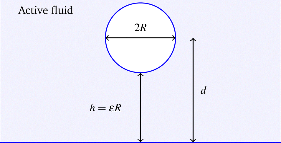
To study wall–particle interactions we use the set up in Fig. 1 consisting of a large circular particle of radius R placed inside in incompressible active nematic at a distance d from a flat uniform wall. The nematic strongly anchors to the wall and surface of the disk, and by symmetry the disk moves in a direction perpendicular to the wall.
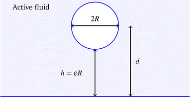 |
| | Fig. 1 A disk of radius R sitting in an active fluid above a wall. The distance between the centre of the disk and the wall is d, and the closest distance between the disk and wall is h = d − R. | |
To model the nematic we use the equations of active nematodynamics describing the coupling of an incompressible velocity field v to the elasticity of the nematic order parameter Q, a symmetric trace-less two tensor1 in the one Frank elastic constant approximation. The two components of the order parameter Qxx = Q1, and Qxy = Q2 may be related to the angle of the nematic director using  , and the scalar order of the nematic by Q02 = Q12 + Q22.
| |  | (1a) |
| | | η∇2v − ∇P + α∇·Q + ∇·σK = 0. | (1b) |
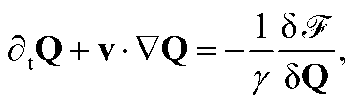
The internal structure of the nematic means that we must account for advection as well as rotation of the nematic director. This is given by the first equation, where
Q relaxes to a minimum of its free energy,
![[scr F, script letter F]](https://www.rsc.org/images/entities/char_e141.gif)
, while being advected and co-rotated by the generalised derivative
Dt.
46 The rate of this relaxation is governed by the rotational viscosity
γ. Alongside the equation for
Q we have the Stokes equations for the fluid, where
P is the pressure, and
η is the viscosity. In addition to the viscous stresses,
σvij =
η(∂
iuj + ∂
jui) −
Pδij there are additional elastic and active stresses from the nematic. The active stresses
σα =
αQ come from the local flows around each nematogen, with
α < 0(>0) for locally contractile (extensile) flows. The elastic stresses
σK derive from the Landau–de Gennes free energy
| |  | (2) |
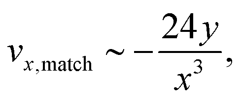
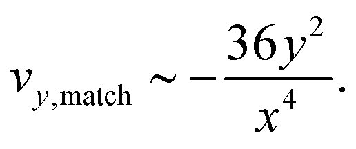
where
K is the elastic constant of the nematic, and
A controls the strength of the nematic order.
47
We make two simplifying approximations, the first being that the distance between the disk and the wall is smaller than the elastic screening length LK2 = A/K. Assuming this we may neglect the A terms in the free energy and take the harmonic approximation48
| |  | (3) |
Importantly this approximation is only valid when there is a wall, and the harmonic approximation to
Q does not work well for an isolated disk.
Secondly, we assume the advective time scale to be much longer than the diffusive time scale. By comparing advective and diffusive terms in eqn (1) we find this is true when h2 ≪ Kη/αγ, where h is the closest distance between the disk and wall. This is the same condition for no spontaneous active flows in a channel of thickness h.49 Although the region under the disk is curved we expect similar qualitative behaviour and so all active flows under the disk ought to be weak.
Assuming these two conditions leads to a simpler, linear set of equations,50
| | | η∇2v − ∇P + α·∇Q + ∇·σK = 0, | (4b) |
| |  | (4c) |
where
H = δ
/δ
Q, and the elastic stress is derived from the harmonic free energy in the Appendix.
As the speed of the disk is as yet unknown, the velocity boundary conditions are zero velocity on the wall, and v = U on the disk. U will later be found with the condition that the disk be force free,51 . The boundary conditions for Q are determined by the anchoring on the wall and disk, which we assume to be strongly planar or normal. From now on we shall work in units where R = 1 unless explicitly stated.
To calculate the hydrodynamic forces on the disk we will first solve for Q, then substitute it into the Stokes equations to find the stresses.
3 Solution
3.1 Nematic field
We assume that the nematic strongly anchors to all surfaces, giving boundary conditions| | Q1 = ±cos![[thin space (1/6-em)]](https://www.rsc.org/images/entities/char_2009.gif) 2θd on the disk, 2θd on the disk, | (5a) |
| | | Q2 = ±sin2θd on the disk, | (5b) |
| | | Q1 = ±1 at the wall and infinity, | (5c) |
| | | Q2 = 0 at the wall and infinity, | (5d) |
where θd is the polar angle centred on the disk. This strong anchoring condition is an approximation, valid when the boundary free energy is negligible compared to the bulk free energy.47 The + gives planar anchoring, and the − normal. Comparing the Q boundary conditions and the definition of the active stress, we see that switching from planar to normal anchoring is equivalent to switching the sign of α. In what follows we shall assume planar anchoring for all calculations.
To solve for Q we use conformal mapping, noting that Laplace's equation is invariant under any conformal map.40 Defining z = x + iy, the relevant conformal mapping is52
| |  | (6) |
where
s depends on
d = 1 +
h through
| |  | (7a) |
| |  | (7b) |
This map takes the blue region in
Fig. 1 to an annulus of inner radius
ρ and outer radius 1, see
Fig. 2. The wall maps to |
w| = 1, the disk to |
w| =
ρ, and the point at infinity to
w = −1.
 |
| | Fig. 2 Conformally mapped domain. The inner circle with radius ρ corresponds to the disk boundary, the outer circle with radius 1 to the wall, and w = −1 to the point at infinity. | |
Defining the complex field, Q = Q1 + iQ2, the solution is found using polar coordinates in the annulus, and is equivalent to a Laurent series in w and ![[w with combining macron]](https://www.rsc.org/images/entities/i_char_0077_0304.gif) ,
,
| |  | (8) |
where the coefficients
cn are
| |  | (9) |
Q in real space is then given by
Q(
w(
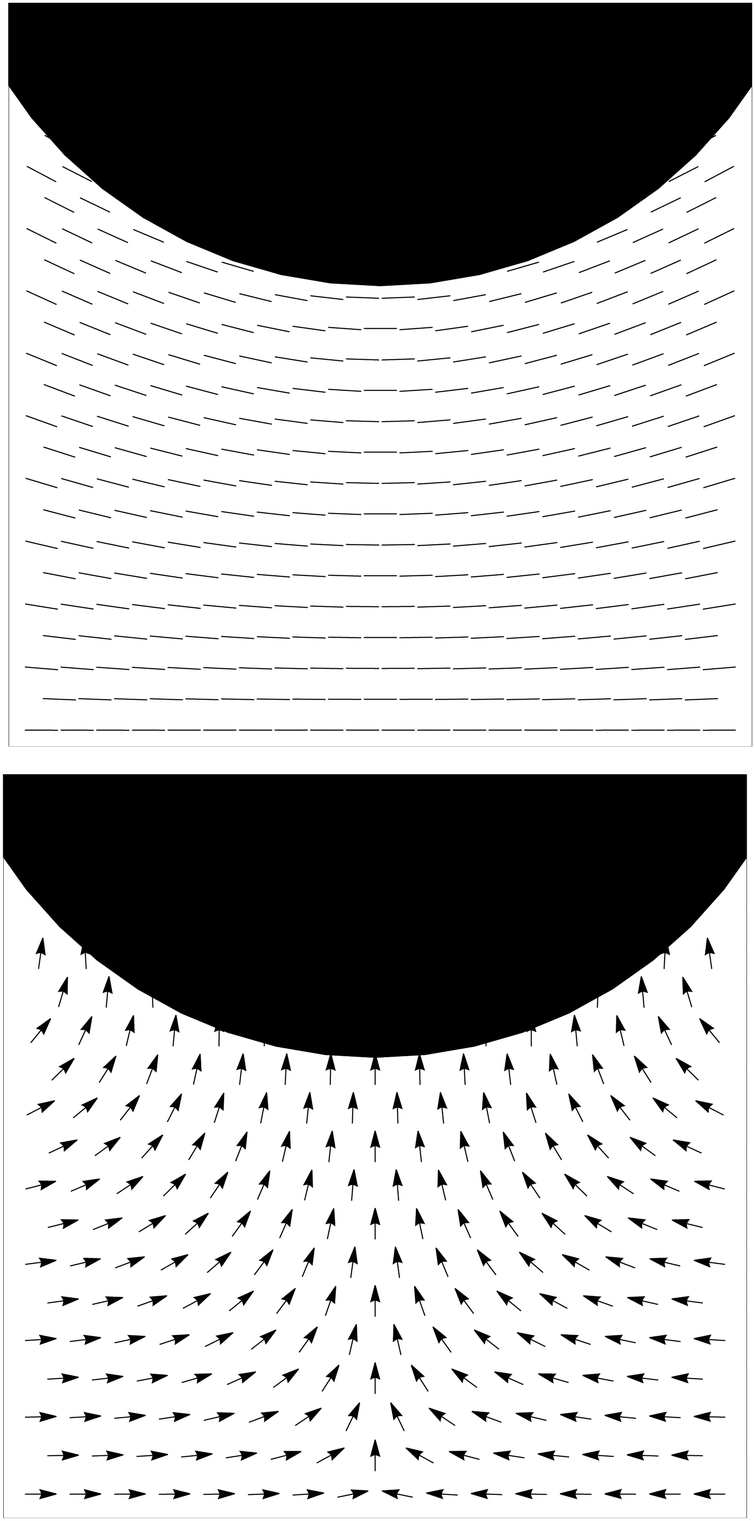
z)). Examining plots of this solution in
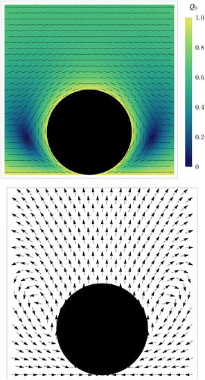
Fig. 3 we see two −1/2 topological defects slightly below the equator of the disk, with their position given by the zeros of
Q0.
53 These are needed to counteract the net +1 topological charge of the disk and represent the lowest energy configuration of defects. The series solution in
(8) may be interpreted as a multipole expansion, with the
nth term corresponding to the
nth multipole.
54 For large disk–wall separations the solution converges rapidly as only the first two terms are needed to capture the quadrupole defect structure.
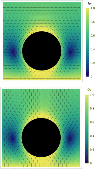 |
| | Fig. 3 Nematic texture around the disk when d = 1.5R. (top) Planar anchoring, (bottom) normal anchoring. | |
3.2 Reciprocal theorem
With Q found we use it to calculate the forces on the disk. To do this we will not need to calculate the velocity field using eqn (4), but shall instead apply the Lorentz reciprocal theorem.55,56 The Lorentz reciprocal theorem relates the stress tensors in two solutions of the Stokes equations in the same domain but with different boundary conditions. To derive the result, consider two copies of the Stokes equations in a domain ![[scr D, script letter D]](https://www.rsc.org/images/entities/char_e523.gif)
| | | η∇2v − ∇P + ∇·Σ = 0, | (10a) |
| | η∇2![[v with combining circumflex]](https://www.rsc.org/images/entities/b_char_0076_0302.gif) − ∇ − ∇![[P with combining circumflex]](https://www.rsc.org/images/entities/i_char_0050_0302.gif) = 0, = 0, | (10b) |
where only one of the copies contains extra stresses Σ, and we have used a carat to distinguish the secondary problem variables. Using these and incompressibility the following integral identity holds| | 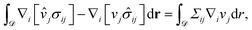 | (11) |
where we have defined the two stress tensors| | | σij = η[∇iuj + ∇jui] − Pδij + Σij, | (12a) |
| | ![[small sigma, Greek, circumflex]](https://www.rsc.org/images/entities/i_char_e111.gif) ij = η[∇iûj + ∇jûi] − δij. ij = η[∇iûj + ∇jûi] − δij. | (12b) |
Applying the divergence theorem to the above integral yields the modified Lorentz reciprocal theorem| |  | (13) |
where ∂ is the boundary of , n is the unit normal to the boundary directed into the fluid domain, and dS is the boundary surface element.
To apply this theorem we use the boundary conditions for v, and choose boundary conditions for to be zero velocity on the wall, and = Û on the disk. Substituting these into eqn (13) we find
| |  | (14) |
where we identified the total (non-viscous) force on the disk
F as the integral of the (non-viscous) stress on its surface.
57 From the (translational) symmetry of the problem we expect the force to be perpendicular to the wall, so choosing
Û =
ey we have
| |  | (15) |
This form of the reciprocal theorem is most helpful to us.
To apply (15) to the active nematic problem we set Σ = αQ + σK (non-viscous part of the stress) and the solve for the secondary velocity using
| | | η∇2 − ∇ = 0, | (16a) |
| | | = 0 on the wall, | (16b) |
| | | = ey on the disk. | (16c) |
We are able to take advantage of the fact that the solution to
eqn (16) is already known, having first been found by Jeffrey and Onishi,
58 and later re-derived by Crowdy using complex analysis.
52 The rest of the paper is devoted to performing the integrals in
eqn (15) a task which is the main technical result of this paper.
3.3 Active force
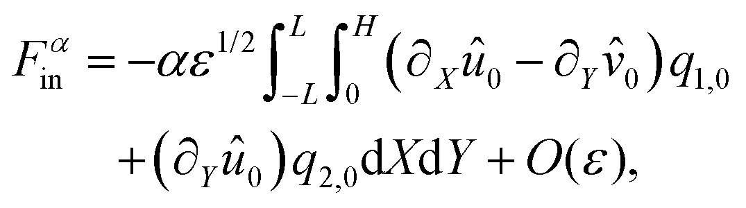
The linearity of eqn (15) allows the (non-viscous) force to be split into an active and elastic contribution F = Fα + FK, where the active contribution is| |  | (17) |
Before performing this integral it is instructive to integrate by parts| |  | (18) |
where we have used the boundary conditions on the disk to factor out the constant Û in the surface integral. The first term on the right hand side is the integral of the active stress over the disk, and so contains no information about stress due to active flows. These are contained in the second term which couples the secondary flow to the driving term in the Stokes equation. It is interesting to contrast with earlier work on particles in active nematics using directors rather Q-tensors. Only the equivalent of the first term was calculated there, as the required secondary solution to the Stokes equations was unknown.36,54
To perform the integral we change to complex coordinates, and integrate in the conformally mapped domain
| |  | (19) |
where
![[v with combining circumflex]](https://www.rsc.org/images/entities/i_char_0076_0302.gif)
=
x +
iy and
![[Q with combining macron]](https://www.rsc.org/images/entities/i_char_0051_0304.gif)
=
Q1 −
iQ2 is the complex conjugate of
Q. Doing the integral yields an active force (with dimensions reinstated)
| |  | (20) |
These results imply that at short distances, planar anchored disks are repelled by active forces in contractile nematics, and attracted in extensile ones. By switching the sign of
α we see the reverse is true in normal anchored nematics. We delay a physical explanation for this till Section 4, where lubrication theory is used to understand the forces origin.
3.4 Elastic force
The elastic contribution to eqn (15) is| |  | (21) |
where we have integrated by parts. Using ∇2Q = 0 and the definition of σK, the second term vanishes. The elastic forces therefore do not affect the flow and are given by the surface integral of σK over the disk| |  | (22) |
To perform the integral we write the stress and surface normal vectors as complex variables σK = σ11 + iσK12 and n = n1 + in2, which after substitution give| |  | (23) |
| |  | (24) |
We calculate this integral using the conformally mapped coordinates, giving| |  | (25) |
where c0 = (ρ − 1)/2logρ, and cn are as defined in (9).
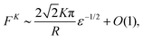
As shown in Fig. 4 (top) the series converges quickly and only two terms in the sum are required for an accurate result; again because two terms are the minimum to capture the quadrupole structure of the defects. The asymptotics for small ε are also dominated by these terms, with the force diverging as ε−1/2 as the disk approaches the wall due to the increasing curvature in the nematic director.
| |  | (26) |
This force is repulsive because the Landau–de Gennes free energy is higher when the disk is closer to the wall and the nematic director is more distorted.
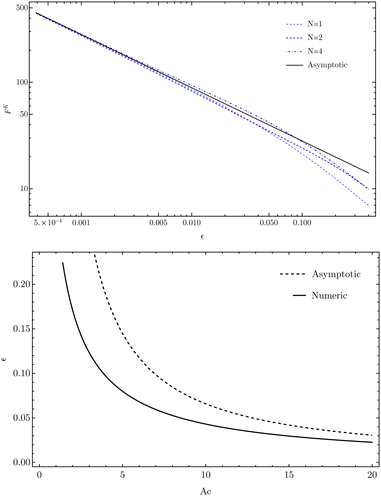 |
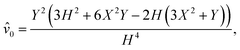
| | Fig. 4 (top) A log–log plot of the elastic force against ε after including N terms in the summation. After two terms there is an adequate result for small ε. (bottom) The steady state value of ε against Ac = αR2/K. The numerical result was calculated using 4 terms in the series for the elastic force, and the asymptotic value is given by ε = 1/2Ac. | |
3.5 Steady state
To calculate the steady state separation we substitute the active and elastic forces into eqn (15), with the requirement that the disk be force free.51 In steady state, the velocity of the disk, U, vanishes, giving the condition FK + Fα = 0. Using this and the sign of the active force, we conclude that planar (normal) anchored disks have a stable steady state height when the nematic is extensile (contractile) as otherwise all forces on the disk are repulsive. Assuming this to be true we numerically solve the force balance condition for ε, with the results shown in Fig. 4. These numerical solutions are compared against the asymptotic result εsteady = K/2αR2, derived by balancing the leading order active and elastic terms.
4 Matched asymptotic analysis
The exact results we have derived give the force on the disk for arbitrary ε, but do not indicate where the force comes from. Is the force dominated by the region under the disk, outside, or is it from both? To investigate this we perform a matched asymptotic analysis of the force integrals (17) and (22).59–61
4.1 Lubrication analysis
Before moving onto a formal asymptotic analysis of the problem we first apply a naive lubrication analysis of eqn (4) by which we mean neglecting horizontal derivatives for vertical ones62| | | η∂y2vx − ∂xP + α∂yQ2 = 0. | (27b) |
The boundary conditions are vx = 0 on the disk and wall; Q2 = 0 on the wall; and Q2 ≈ 2θd on the wall, where we have expanded the boundary conditions for small disk angle. The distance between the disk and the wall is approximately h(x) = ε + x2/2, and the disk angle is h′(x) = x. Using these we find Q2 = 2yx/h, and a horizontal velocity| |  | (28) |
where P′ = ∂xP. If the disk moves upwards at velocity U then flux arguments give the pressure as| |  | (29) |
Unfortunately the active contribution diverges logarithmically. This means that this lubrication theory must be matched to an outer region to get a finite answer. This logarithmic divergence was also found in the study of active nematic droplets, however it did not cause problems because of the finite drop size.62 Substituting this pressure into the velocity equation, we find all active flow terms cancel out, meaning that the dominant active effect is from an active pressure rather than active flows. This justifies our earlier assumption of neglecting advection at leading order. Interestingly, integrating the pressure under the disk, we find the active force active to be| |  | (30) |
i.e. the finite part of the active pressure force gives the correct leading order result.
One may wonder why we referred to the lubrication analysis above as ‘naïve’. This is because a more detailed asymptotic analysis reveals that all Q terms are irrelevant to leading order in ε. This more detailed asymptotic analysis is given next.
4.2 Inner expansion
To regularise the divergent terms in (30) we use a matched asymptotic analysis and split the domain into an inner and outer region. We then solve the problem separately in these regions, before matching them together. The inner region corresponds to a small area under the disk as in Fig. 5. The surface of the disk is at y = h(x), where| |  | (31) |
From this expansion we see that the inner variables are defined by y = εY, and x = ε1/2X, in which| |  | (32) |
and the angle of the disk is θd = h′(x) ∼ ε1/2H′(X). Substituting these scaled variables into eqn (4), (5) and (16) leads us to pose the expansions| | | Q1 = q1,0 + εq1,1 + …, | (33a) |
| | | Q2 = ε1/2q2,0 + ε3/2q2,1 + …, | (33b) |
| | | x = ε−1/2û0 + ε1/2û1 + …, | (33c) |
| | | = ε−3/20 + ε−1/21 + …, | (33e) |
where the scaling of x compared to y is from incompressibility. Substitution of these back into eqn (4) and (16) yields the leading order equations| | | η∂Y2û0 − ∂X0 = 0, | (34a) |
| | | ∂Y0 = 0, | (34b) |
Solving these with appropriate boundary conditions (5) and (16) gives| |  | (35b) |
| |  | (35c) |
| |  | (35d) |
which are shown in Fig. 6. As with the naive analysis, these inner solutions alone give a divergent force. We now calculate the outer solution and match them together.
 |
| | Fig. 5 Inner and outer regions for matched asymptotic expansion. In the outer region the disk is touching the wall. In the inner region the height of the disk above the wall is parameterised as y = h(x), where x is the coordinate along the wall. | |
 |
| | Fig. 6 Nematic director and secondary velocity in the inner region. (top) The nematic director is parallel anchored to all surfaces with Q0 ≈ 1 everywhere. (bottom) The velocity is zero on the wall, vertically upwards on the disk, and has a stagnation point at the origin. | |
4.3 Outer expansion
The outer region corresponds to ε = 0, or when the disk touches the wall. To solve for Q and we will apply conformal mapping, defining the variable ζ = μ + iξ = −2/z, with μ,ξ real.41 Under this map the region outside the disk transforms to the channel μ ∈ (−∞,∞), ξ ∈ [0,1], where the plane wall maps to ξ = 0, the disk to ξ = 1, and the point at infinity to μ = ξ = 0.
We begin with Q, for which the boundary conditions (5) translate to
| |  | (36b) |
and we have used
Q =
Q1 +
iQ2. We solve Laplace's equation by Fourier transform in the
μ direction, with the solution
| |  | (37) |
This can be integrated63 to give
| |  | (38) |
where
ψ is the digamma function, and
ψ(1) its derivative. This solution, shown in
Fig. 7 (top), exhibits two −1/2 topological defects slightly below the equatorial line parallel to the director orientation far from the inclusion at positions (
x1/2,
y1/2) ≈ (±1.484, 0.876)
R. This can be compared to a disk in free space where the defects are equatorial and their position is known to be
x1/2 ≈ 1.236
R,
64 and so we see that the displacement of the defect from the disk's equatorial line is due to the interaction between the disk and the wall.
39 In contrast, we think that the larger distance for the
Q-tensor model is due to the harmonic approximation of the Landau–de Gennes free energy
(2). This is because the higher order terms control the defect size, with defects being larger for smaller values of
A.
39,53,64
 |
| | Fig. 7 Nematic director and secondary velocity in the outer limit. (top) The nematic director is parallel anchored to all surfaces, becoming uniformly horizontal at infinity. (bottom) The velocity diverges at the point where the disk touches the wall and so we only plot its direction. | |
With Q in hand we turn to the outer velocity of the secondary problem, , which solves the ordinary Stokes equations with boundary conditions:
| | | ûx + iûy = 0 on the wall, | (39a) |
| | | ûx + iûy = i on the disk, | (39b) |
| | | ûx + iûy = 0 at infinity. | (39c) |
There is an inconsistency in the boundary conditions where the disk touches the wall, so we search for solutions that are valid everywhere except this point. As far as we are aware the solution to this problem does not yet exist in the literature.
We begin by writing the stream function as combination of two analytic functions65
| | ![[small psi, Greek, circumflex]](https://www.rsc.org/images/entities/i_char_e0b6.gif) = Im[ = Im[![[z with combining macron]](https://www.rsc.org/images/entities/i_char_007a_0304.gif) f(z) + g(z)], f(z) + g(z)], | (40) |
from which the complex velocity is given by
| |  | (41) |
where ′ denotes a
z derivative. Defining
g′(
z) =
G(
z) and converting to
ζ coordinates yields
| |  | (42) |
where
f(
ζ) =
f(
ζ(
z)). On the disk
![[small zeta, Greek, macron]](https://www.rsc.org/images/entities/i_char_e0c7.gif)
=
ζ, and on the wall
=
ζ − 2
i, therefore the boundary conditions may be re-written as two functional relations
| | −ζf′(ζ) + G(ζ) − ![[f with combining macron]](https://www.rsc.org/images/entities/i_char_0066_0304.gif) (ζ) = 0, (ζ) = 0, | (43a) |
| |  | (43b) |
where

. These two equations only depend on analytic functions of
ζ, and therefore hold over the entire channel. Subtracting one from the other we arrive at a functional relation for
f(
ζ)
| | | 2iζf′(ζ) + (2i − ζ)[(ζ) − (ζ − 2i) + i] = 0. | (44) |
This is solved by the polynomial
| |  | (45) |
and
(45) into
(43) determines
G(
ζ) to be
| |  | (46) |
With
f(
ζ) and
G(
ζ) we have the stream function and hence the full secondary velocity field. This solution, shown in
Fig. 7 (bottom), satisfies all the boundary conditions and although regular in the
ζ plane, diverges at the touching point when converting back to real coordinates.
To check that our inner and outer solutions match we take the outer limit of the inner expansion and compare it to the inner limit of the outer expansion.61 We find they match, with the overlapping function given by
| |  | (47b) |
| |  | (47c) |
| |  | (47d) |
4.4 Active force
The active force is given by the integral of fα = −αQij∇ij over the entire domain outside the disk. To see why we need asymptotic matching let us calculate the inner contribution to this force, which to leading order is given by| | 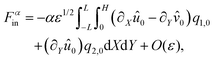 | (48) |
where L is some length at which the inner solution fails. In many problems this integral converges to a finite value as L tends to infinity and the outer problem can be ignored.58,59 In our case the integral diverges, implying that we must match to an outer region| |  | (49) |
To perform matching we construct a globally valid asymptotic approximation to fα which is then integrated over the entire domain. As fα combines two functions it mixes various powers of ε, which, although not a problem in the outer region (ε = 0), complicates matters in the inner region. To leading order fαinner is given by eqn (48) converted back to outer, (x,y) coordinates.
To match fαinner to the outer integrand, fαouter, we take the outer limit of the inner expansion and the inner limit of the outer expansion.61 Comparing the two we find an overlapping contribution
| |  | (50) |
which upon integration over the inner region gives
Fαoverlap ∼ −4
αε1/2L +
O(
L−3),
i.e. the overlap is responsible for the divergence. This term will appear in both the inner and outer contributions to the active force but with a relative minus sign between them, cancelling when the two contributions are added.
We now construct globally valid approximation according to
| | | fαuniform = fαin + fαout − fαoverlap, | (51) |
using which the total active force is

, where we integrate using the conformal coordinates defined in Section 3.1. The result is
| |  | (52) |
which agrees with the exact result from
eqn (20), and we have succeeded in regularising the naive result in
(30). This result indicates that the leading order contribution to the active force comes from the curvature in the nematic director in a small region under the disk.
4.5 Elastic force
The elastic force is calculated as a surface integral using eqn (22). The leading order inner contribution is| |  | (53) |
Substituting (35) gives the elastic force| |  | (54) |
which converges to a finite value as L tends to infinity and confirms the exact result of eqn (26). Again, this result shows that the leading order contribution to the elastic force is due to the small region of nematic curvature under the disk.
5 Comparison of Q-tensor and nematic director
Numerical studies of disks near walls in two dimensional passive liquid crystals indicate that as the disk approaches the wall, the topological defects also move closer.39 Although these studies were based upon minimising the full Landau de-Gennes free energy (2), for non-zero A, our analysis indicates that some of the qualitative behaviour, such as defects moving below the equator, may be captured by setting A to zero.
To understand the location and impact of the topological defects, it is worth considering the opposite limit to what we have done so far, i.e. letting the nematic become very stiff. This corresponds to letting the A parameter in eqn (2) tend to infinity such that the magnitude of the Q-tensor is fixed at one. In this limit it is known that minimising the full Landau de-Gennes free energy is equivalent to solving ∇2θ = 0, where θ is the angle of the nematic director field.47 Using the director, topological defects correspond to singularities in the angle and must be added in by hand.
It is interesting to see how our analysis with A = 0 differs. Unfortunately we do not find it possible to use θ when the disk is above the wall due to the multiple connectivity of the domain. However when the disk is touching we may apply the Fourier transform techniques of Section 4.3. Following the same steps we used to find Q gives
| |  | (55) |
where π/2 may be added to switch from planar to normal anchoring. Note that
θ diverges at the point where the disk touches the wall. Interestingly this solution has no visible topological defects though the disk still has a net +1 charge, and our
Q tensor based solution had defects. As shown in
Fig. 8, this appears to be because the two −1/2 topological defects move under and around the disk as it approaches, merging to create a −1 defect at the point of contact. This only happens in the
θ description because the defects are point-like objects, whereas in in the
Q tensor description the defects always have a finite extent. Note that in the inner region, the nematic textures found using either the
Q-tensor or director angle are the same, and so the leading order active and elastic forces are identical.
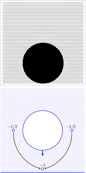 |
| | Fig. 8 Director angle in the outer limit. (top) The nematic director is parallel anchored to all surfaces, becomes uniformly horizontal at infinity, and diverges where the disk touches the plane. (bottom) Schematic illustration of what happens to the −1/2 topological defects as the disk approaches and then touches the wall. | |
6 Conclusions
We have shown that a disk immersed in active liquid crystals can be attracted or repelled by walls depending on a combination of activity and anchoring conditions. In particular, planar (normal) anchored disks are repelled (attracted) by active forces when the nematic is contractile (extensile). When the disk is sufficiently close to the wall and the flows are sufficiently slow, we can obtain exact expressions for the effective forces by combining tools from complex analysis and the Lorentz reciprocal theorem. This theorem allowed us to avoid solving the Stokes equations forced by active stresses, and instead use a solution to the Stokes equations when activity was zero. We then applied a matched asymptotic analysis to study the same problem when the disk was very near the wall which revealed that the leading order contribution to the force came from the small region between the disk and the wall.
Our calculations are done in the strong elastic limit when the active nematic affects the fluid velocity field but in which the flow does not affect the nematic director field. Nevertheless we expect qualitatively similar behaviour even when back-flow is relevant. These results can be experimentally tested by placing floating disks into two dimensional active nematic films.20,23,27,66 Our results will be important when the disks are close to the wall, or each other, whereas active turbulence will dominate when they are far apart. As such, these effects will be important when studying dense suspensions of colloidal disks, and by combining activity and anchoring can perhaps be used to enhance (or reduce) the self-assembly of active nematic colloids, as in ref. 33. At very high activity, the nematic director field far from the wall becomes highly disordered with associated hydrodynamic flows (this is sometimes called “active turbulence”) characterised by a typical lengthscale governed by the balance of activity, elasticity and dissipation. We expect that our results here will be relevant when the separation between the disk and the wall is small compared to this lengthscale. Far from the wall, in this highly active regime, the disks will be pushed around by the chaotic flow.9 This problem is not suitable to detailed mathematical analysis of the type we do here and is best studied numerically. However it is possible that the fluctuating forces on the disks could be approximated for by a random force with a spectrum chosen to match that of the disordered flow.8,67 This is a possible direction for future work in this field.
We must not forget that typically in these experiments20,23,27,66 the two dimensional active nematic film lies between two other fluids and to be accurately modelled, one must include the fluid dissipation from the three-dimensional fluids above and below the film, a problem that was first popularised by Saffman and Delbrück.68 It is well known that this implies that there is two-dimensional Stokes behaviour only on length-scales much smaller than the Saffman–Delbrück length.68–73 Hence our calculations are valid only when this length is larger than all the length-scales in the problem. Including the effect of a finite Saffman–Delbrück length makes it hard to use complex analytic techniques to solve for the velocity field and one will only be able to obtain approximate results using the matched asymptotic techniques outlined above. It is possible to go beyond the strong anchoring limit by adding a surface anchoring term in the free energy (2) to account for the finite anchoring strength of the nematic.47 This alters the boundary conditions on the disk and wall (5), and hence makes it difficult to use complex analytic techniques.42 We leave this for the future.
We foresee two further extensions of this work: the first being the problem of two disks meeting each other, rather than one approaching a wall; the second being the same problem in three dimensions, where complex analytic techniques could not be used. For the first problem, the secondary velocity field is known,74 but it is difficult to solve for Q. This is a known problem, as even solving Laplace's equation for a scalar field with constant boundary conditions on two disks while going to zero at infinity is famously hard.75,76 For the second problem of a sphere approaching a wall, even the secondary velocity is difficult as one must use bi-spherical coordinates.59,77 Moreover, the nematic director configuration is much trickier as there is not a unique director field that is planar or normal anchored everywhere to the sphere.29
Author contributions
LN, JE, TBL designed the problem, LN performed the research and LN, JE, TBL analysed the results and wrote the manuscript.
Data availability
The code for the nematic texture and velocity field is available at https://doi.org/10.5281/zenodo.13354366.
Conflicts of interest
There are no conflicts to declare.
Appendix: elastic stresses
Using Q, the full equations of active nematics are78| |  | (56a) |
| | | η∇2v − ∇P + α∇·Q + ∇·σK = 0. | (56b) |
We neglect co-rotation and flow aligning terms as their stress tensors are zero if ∇2Q = 0. We work with a simplified free energy| |  | (57) |
but the same method holds for more complicated free energies. To derive the elastic stress we follow78 and calculate the rate of change of free energy.| |  | (58) |
where we have integrated by parts and dropped a surface term, assuming that Q has fixed boundary conditions on any surface. We now replace ∂tQ using (56)| |  | (59) |
Now consider the total change for a small time  , and balance the change in free energy due to the flow with the one caused by stress.53
| |  | (60) |
Comparing each term we find a total stress
| |  | (61) |
Acknowledgements
The authors acknowledge helpful discussions with O. Schnitzer. LN and TBL would like to thank the Isaac Newton Institute for Mathematical Sciences, Cambridge, for support and hospitality during the programme New statistical physics in living matter, where part of this work was done. This work was supported by EPSRC grants EP/R014604/1 and EP/T031077/1.
Notes and references
- M. C. Marchetti, J. F. Joanny, S. Ramaswamy, T. B. Liverpool, J. Prost, M. Rao and R. A. Simha, Rev. Mod. Phys., 2013, 85, 1143–1189 CrossRef.
- S. Ramaswamy, Annu. Rev. Condens. Matter Phys., 2010, 1, 323–345 CrossRef.
- T. Vicsek, A. Czirók, E. Ben-Jacob, I. Cohen and O. Shochet, Phys. Rev. Lett., 1995, 75, 1226–1229 CrossRef.
- J. Toner and Y. Tu, Phys. Rev. E: Stat. Phys., Plasmas, Fluids, Relat. Interdiscip. Top., 1998, 58, 4828 CrossRef.
- J. Toner, Y. Tu and S. Ramaswamy, Ann. Phys., 2005, 318, 170–244 Search PubMed.
- Y. Fily and M. C. Marchetti, Phys. Rev. Lett., 2012, 108, 235702 CrossRef.
- M. E. Cates and J. Tailleur, Annu. Rev. Condens. Matter Phys., 2015, 6, 219–244 CrossRef.
- R. Alert, J.-F. Joanny and J. Casademunt, Nat. Phys., 2020, 16, 682–688 Search PubMed.
- R. Alert, J. Casademunt and J.-F. Joanny, Annu. Rev. Condens. Matter Phys., 2022, 13, 143–170 Search PubMed.
- A. Creppy, O. Praud, X. Druart, P. L. Kohnke and F. Plouraboué, Phys. Rev. E: Stat., Nonlinear, Soft Matter Phys., 2015, 92, 032722 CrossRef PubMed.
- J. Dunkel, S. Heidenreich, K. Drescher, H. H. Wensink, M. Bär and R. E. Goldstein, Phys. Rev. Lett., 2013, 110, 228102 CrossRef PubMed.
- G. Gompper, R. G. Winkler, T. Speck, A. Solon, C. Nardini, F. Peruani, H. Löwen, R. Golestanian, U. B. Kaupp and L. Alvarez,
et al.
, J. Phys.: Condens. Matter, 2020, 32, 193001 CrossRef.
- C. Maggi, J. Simmchen, F. Saglimbeni, J. Katuri, M. Dipalo, F. De Angelis, S. Sanchez and R. Di Leonardo, Small, 2016, 12(4), 446–451 CrossRef PubMed.
- K. J. Bishop, S. L. Biswal and B. Bharti, Annu. Rev. Chem. Biomol. Eng., 2023, 14, 1–30 CrossRef PubMed.
- C. P. Goodrich and M. P. Brenner, Proc. Natl. Acad. Sci. U. S. A., 2017, 114, 257–262 CrossRef PubMed.
- A. Zöttl and H. Stark, J. Phys.: Condens. Matter, 2016, 28, 253001 CrossRef.
- A. Zöttl and H. Stark, Annu. Rev. Condens. Matter Phys., 2023, 14, 109–127 CrossRef.
- I. S. Aranson, Phys.-Usp., 2013, 56, 79 CrossRef CAS.
- A. Aubret, Q. Martinet and J. Palacci, Nat. Commun., 2021, 12, 6398 CrossRef CAS.
-
S. Ray, J. Zhang, P. Atzberger, C. Marchetti and Z. Dogic, APS March Meeting Abstracts, 2022, p. W20.007 Search PubMed.
- S. Mallory, C. Valeriani and A. Cacciuto, Phys. Rev. E: Stat., Nonlinear, Soft Matter Phys., 2014, 90, 032309 CrossRef.
- R. A. Simha and S. Ramaswamy, Phys. Rev. Lett., 2002, 89, 058101 CrossRef PubMed.
- A. Doostmohammadi, J. Ignés-Mullol, J. M. Yeomans and F. Sagués, Nat. Commun., 2018, 9, 3246 CrossRef PubMed.
- D. Dell’Arciprete, M. L. Blow, A. T. Brown, F. D. Farrell, J. S. Lintuvuori, A. F. McVey, D. Marenduzzo and W. C. Poon, Nat. Commun., 2018, 9, 4190 CrossRef PubMed.
- F. Julicher, K. Kruse, J. Prost and J. Joanny, Phys. Rep., 2007, 449, 3–28 CrossRef.
- D. Needleman and Z. Dogic, Nat. Rev. Mater., 2017, 2, 1–14 Search PubMed.
- T. Sanchez, D. T. Chen, S. J. DeCamp, M. Heymann and Z. Dogic, Nature, 2012, 491, 431–434 CrossRef CAS PubMed.
- N. D. Mermin, Rev. Mod. Phys., 1979, 51, 591 CrossRef CAS.
- H. Stark, Phys. Rep., 2001, 351, 387–474 CrossRef CAS.
- P. Poulin, H. Stark, T. Lubensky and D. Weitz, Science, 1997, 275, 1770–1773 CrossRef PubMed.
- P. Poulin and D. Weitz, Phys. Rev. E: Stat. Phys., Plasmas, Fluids, Relat. Interdiscip. Top., 1998, 57, 626 CrossRef.
- I. Mušević, Materials, 2017, 11, 24 CrossRef PubMed.
- I. Mušević and M. Škarabot, Soft Matter, 2008, 4, 195–199 RSC.
- M. Škarabot, M. Ravnik, S. Žumer, U. Tkalec, I. Poberaj, D. Babić, N. Osterman and I. Mušević, Phys. Rev. E: Stat., Nonlinear, Soft Matter Phys., 2007, 76, 051406 CrossRef PubMed.
- S. Ray, J. Zhang and Z. Dogic, Phys. Rev. Lett., 2023, 130, 238301 CrossRef PubMed.
- A. J. Houston and G. P. Alexander, New J. Phys., 2023, 25, 123006 CrossRef.
- B. Loewe and T. N. Shendruk, New J. Phys., 2022, 24, 012001 CrossRef.
- T. Yao, Ž. Kos, Q. X. Zhang, Y. Luo, E. B. Steager, M. Ravnik and K. J. Stebe, Sci. Adv., 2022, 8, eabn8176 CrossRef.
- N. Silvestre, P. Patrcio, M. Tasinkevych, D. Andrienko and M. T. da Gama, J. Phys.: Condens. Matter, 2004, 16, S1921 CrossRef.
-
Z. Nehari, Conformal mapping, Courier Corporation, 2012 Search PubMed.
-
H. Kober, Dictionary of Conformal Representations, Dover, New York, 1957, vol. 2 Search PubMed.
-
T. G. Chandler and S. E. Spagnolie, arXiv, 2023, preprint, arXiv:2311.17708 Search PubMed.
-
D. Crowdy, Solving problems in multiply connected domains, SIAM, 2020 Search PubMed.
- V. M. Batista, M. L. Blow and M. M. T. da Gama, Soft Matter, 2015, 11, 4674–4685 RSC.
- T. N. Shendruk, A. Doostmohammadi, K. Thijssen and J. M. Yeomans, Soft Matter, 2017, 13, 3853–3862 RSC.
-
A. N. Beris and B. J. Edwards, Thermodynamics of flowing systems: with internal microstructure, Oxford University Press, USA, 1994 Search PubMed.
-
P.-G. de Gennes and J. Prost, The Physics of Liquid Crystals, Clarendon Press, Oxford, 2nd edn, 2013 Search PubMed.
- S. P. Thampi, A. Doostmohammadi, R. Golestanian and J. M. Yeomans, Europhys. Lett., 2015, 112, 28004 CrossRef.
- R. Voituriez, J.-F. Joanny and J. Prost, Europhys. Lett., 2005, 70, 404 CrossRef.
- A. Loisy, J. Eggers and T. B. Liverpool, Phys. Rev. Lett., 2019, 123, 248006 CrossRef.
- E. Lauga and T. R. Powers, Rep. Prog. Phys., 2009, 72, 096601 CrossRef.
- D. Crowdy, Int. J. Non Linear Mech., 2011, 46, 577–585 CrossRef.
-
P. M. Chaikin, T. C. Lubensky and T. A. Witten, Principles of condensed matter physics, Cambridge University Press, Cambridge, 1995, vol. 10 Search PubMed.
- A. J. Houston and G. P. Alexander, Front. Phys., 2023, 11, 222 Search PubMed.
- H. Masoud and H. A. Stone, J. Fluid Mech., 2019, 879, P1 CrossRef.
-
S. Kim and S. J. Karrila, Microhydrodynamics: Principles and Selected Applications, Dover Publications, Mineola, NY, 2005 Search PubMed.
-
G. K. Batchelor, An Introduction to Fluid Dynamics, Cambridge Univ. Press, Cambridge, 14th edn, 2010 Search PubMed.
- D. J. Jeffrey and Y. Onishi, Q. J. Mech. Appl. Math., 1981, 34, 129–137 CrossRef.
- M. Cooley and M. O'neill, Mathematika, 1969, 16, 37–49 CrossRef.
-
C. M. Bender and S. A. Orszag, Advanced mathematical methods for scientists and engineers I: Asymptotic methods and perturbation theory, Springer Science & Business Media, 2013 Search PubMed.
-
E. J. Hinch, Perturbation Methods, Cambridge University Press, 1991 Search PubMed.
- J.-F. Joanny and S. Ramaswamy, J. Fluid Mech., 2012, 705, 46–57 CrossRef.
-
I. S. Gradshteyn and I. M. Ryzhik, Table of integrals, series, and products, Academic Press, 2014 Search PubMed.
- M. Tasinkevych, N. Silvestre, P. Patricio and M. Telo da Gama, Eur. Phys. J. E: Soft Matter Biol. Phys., 2002, 9, 341–347 CrossRef CAS PubMed.
- S. Richardson, J. Fluid Mech., 1968, 33, 475–493 CrossRef.
- J. Hardoüin, R. Hughes, A. Doostmohammadi, J. Laurent, T. Lopez-Leon, J. M. Yeomans, J. Ignés-Mullol and F. Sagués, Commun. Phys., 2019, 2, 121 CrossRef.
- L. Giomi, Phys. Rev. X, 2015, 5, 031003 Search PubMed.
- P. G. Saffman, J. Fluid Mech., 1976, 73, 593–602 CrossRef.
- B. Martínez-Prat, R. Alert, F. Meng, J. Ignés-Mullol, J.-F. Joanny, J. Casademunt, R. Golestanian and F. Sagués, Phys. Rev. X, 2021, 11, 031065 Search PubMed.
- R. Matas-Navarro, R. Golestanian, T. B. Liverpool and S. M. Fielding, Phys. Rev. E: Stat., Nonlinear, Soft Matter Phys., 2014, 90, 032304 CrossRef PubMed.
- A. Levine, T. Liverpool and F. MacKintosh, Phys. Rev. E: Stat., Nonlinear, Soft Matter Phys., 2004, 69, 1–10 CrossRef.
- D. K. Lubensky and R. E. Goldstein, Phys. Fluids, 1996, 8, 843–854 CrossRef.
- H. A. Stone and A. Ajdari, J. Fluid Mech., 1998, 369, 151–173 CrossRef.
- S. Wakiya, J. Phys. Soc. Jpn., 1975, 39, 1603–1607 CrossRef.
-
A. Darevski, The electrostatic field of a split phase, 1958 Search PubMed.
-
J. Lekner, Electrostatics of Conducting Cylinders and Spheres, AIP Publishing, 2021 Search PubMed.
- H. Brenner, Chem. Eng. Sci., 1961, 16, 242–251 CrossRef.
- M. E. Cates and E. Tjhung, J. Fluid Mech., 2018, 836, P1 CrossRef.
|
| This journal is © The Royal Society of Chemistry 2024 |
Click here to see how this site uses Cookies. View our privacy policy here. 
 Open Access Article
 This Open Access Article is licensed under a
  *ab,
Jens
Eggers
*ab,
Jens
Eggers
 , and the scalar order of the nematic by Q02 = Q12 + Q22.


 . The boundary conditions for Q are determined by the anchoring on the wall and disk, which we assume to be strongly planar or normal. From now on we shall work in units where R = 1 unless explicitly stated.


 . These two equations only depend on analytic functions of ζ, and therefore hold over the entire channel. Subtracting one from the other we arrive at a functional relation for f(ζ)


 , where we integrate using the conformal coordinates defined in Section 3.1. The result is


 , and balance the change in free energy due to the flow with the one caused by stress.53
