
 Open Access Article
 This Open Access Article is licensed under a
 Creative Commons Attribution 3.0 Unported Licence
Hydrodynamically induced aggregation of two dimensional oriented active particles†
Roee
Bashan
and
Naomi
Oppenheimer
 *
*
School of Physics and Astronomy and the Center for Physics and Chemistry of Living Systems, Tel Aviv University, Israel. E-mail: naomiop@gmail.com
First published on 18th March 2024
Abstract
We investigate a system of co-oriented active particles interacting only via hydrodynamic and steric interactions in a two-dimensional fluid. We offer a new method of calculating the flow created by any active particle in such a fluid, focusing on the dynamics of flow fields with a high-order spatial decay, which we analyze using a geometric Hamiltonian. We show that when the particles are oriented and the flow has a single, odd power decay, such systems lead to stable, fractal-like aggregation, with the only exception being the force dipole. We discuss how our results can easily be generalized to more complicated force distributions and to other effective two-dimensional systems.
Out-of-equilibrium ensembles, both biological and artificial, are often suspended in a fluid. Many times, these active systems have lower dimensions.1–3 A prominent example is a cell membrane—an effective two-dimensional (2D) fluid in which both passive and active proteins are immersed.4 Active membrane proteins act as either rotary proteins, such as ATP synthase,5,6 or as shakers—particles that are not self-propelled but apply active forces on the membrane due to conformational changes, polymerization, or reorganization.7 Artificial 2D systems are also widespread, such as active colloids driven by a chemical reaction,8–10 by light11,12 or by an external magnetic field.13 Particle dynamics can be dominated by complex interactions (e.g. by electrostatics, capillary forces or an external field),14,15 or by purely hydrodynamic flows.16–20 In all the above systems, understanding the connection between flow and structure is crucial.
The flow created by an active particle can be described by a multipole expansion (similar to electrostatics). Far away from the particle, the leading order of the flow, the stokeslet, is given by the total force the particle applies. Closer to the particle, higher multipole contributions start to dominate. First, the force dipole, which could be divided to the rotlet,5,21–24 and the stresslet.25–28 Closer still, the quadrupolar term is significant, then the octopole, and so forth.29,30 Thus, by first finding the effect of a single point-force, the so-called Green's function of the problem, we can derive the general flow response. This procedure applies even when there is no net force, in which case the higher orders dominate at larger distances.
In this work, we explore the dynamics of suspended particles in a 2D viscous fluid in which particles are all oriented along the same direction and interact only via the flow they create at their boundary and steric interactions. We review how the multipole terms mentioned above are often calculated from the stokeslet, but then, we focus on improving the common procedure, making higher-order terms easier to use and calculate. We show that, in many cases, namely for all terms of the multiple expansion with an odd power decay, the dynamics could be described by a Hamiltonian. This Hamiltonian is geometric in nature, with the conjugate variables being xi and yi, the position of the ith particle. Phase-space in such cases corresponds to configurational-space. Thus, by limiting possible paths in phase-space we can determine the steady-state distributions such active particles can take. We prove that, in many cases, particles aggregate. In particular, in all far-field limits, which are dominated by a single multipole term with an odd power decay, the only exceptions being the rotlet and the stresslet. We corroborate our findings by simulating particles that interact by an octopolar force distribution. Fig. (1) illustrates our key finding: a pure multipole force distribution leads to particle aggregation. Moreover, we claim that our findings can be applied to more general 2D cases—both for calculating high-order interactions in more complex fluids, and for understanding their resulting dynamics in many-particle ensembles.
 | ||
| Fig. 1 Snapshots of a simulation of 500 active particles with an octopole force distribution (i.e., the velocity decays as 1/r3). Particles are initialized randomly in a 60 × 60 box; All particles are oriented along the x axis. The particles collide quickly only due to hydrodynamic interactions and form small clusters. At long times, clusters also collide, creating larger clusters. Finally, The particles form a single, fractal-like, cluster organized in a 45° angled square lattice. | ||
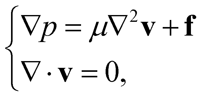
The Reynolds number of a flow, Re = ρUL/μ, is the ratio between the inertia of the fluid and the viscous forces in its flow, where ρ is the fluid's density, μ is its viscosity, U is the characteristic velocity and L the characteristic length. For microswimmers in biological systems, the Reynolds number is small, as the characteristic lengths are microscopic. In the low Reynolds number limit, the inertia is thus negligible, and the flow velocity v(r) (where r = (x,y) is the 2D position vector) is governed by the Stokes equations,
 | (1) |
 | (2) |
| v = F·G + D2 : ∇G +⋯+ DN∇Ⓝ⊗N−1G +⋯ | (3) |
 | (4) |
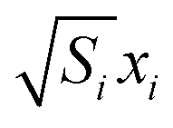
Let us now consider a fluid in which an active particle is immersed. The particle is propagated by the flow only (we will later add steric interactions for the sake of simulations), and so its position is given by a simple equation of motion ṙ = v(r). Since the flow is incompressible and has no sources of mass (eqn (1)), it can be described by a scalar field ψ called the stream function. In 2D, ∇ × (ψẑ) = v ≡ ∇⊥ψ, where ∇⊥ = −ẑ × ∇ = ![[x with combining circumflex]](https://www.rsc.org/images/entities/i_char_0078_0302.gif) ∂y − ŷ∂x. In the case of a flock of similar particles, all with the same orientation, each with strength Si, the stream function created by all particles is a simple superposition,
∂y − ŷ∂x. In the case of a flock of similar particles, all with the same orientation, each with strength Si, the stream function created by all particles is a simple superposition,  . The dynamics of the particles could be described by a geometric Hamiltonian
 | (5) |
 and
and  being conjugate variables. Such a Hamiltonian description has been useful for point vortices in an ideal fluid32,33 and also, more recently, in viscous systems.26,34–37 However, this formalism only holds when ψ is an even function of r. An odd component of ψ will cancel out in the (symmetric) summation, and H would be identically zero. In the rest of this work, we will mostly use the case where the particles are identical, i.e. Si = 1.
The rest of the paper is organized as follows. In Section 1 we will derive the 2D flow created by an active particle with any force distribution on its surface. In Section 2, we will derive the dynamics of two similar particles oriented along the same direction. As an example, we will show that when the force distribution is octopolar, dominated by D4, particles will collide at a finite time. We will then prove that, except for a force-dipole, all interactions of a single, even, multipole term lead to aggregation in the two-particle system. We will also discuss more general interactions. Our arguments will also be applicable to other similar systems with flow fields not described by the equations of flow above. In Section 3, we will claim that the two-particle case also applies to an ensemble of many particles and show a simulation resulting in aggregation.
1 Flow due to a single particle
Here, we will derive the stream function generated by a general active particle in a 2D viscous fluid. For simplicity, we will assume a circular particle with a radius R, applying a surface force on the fluid at its boundary. However, the choice that forces are only applied on a circle does not limit the result of the stream function, and all the solutions in eqn (3) will appear here as well (see ESI† for more details). Taking the curl of the first equation in eqn (1), and writing the velocity in terms of ψ, we arrive at an equation for the stream function,| ∇2∇2ψ = −∇⊥·f = ẑ·(∇ × f). | (6) |
The force is only present at the surface of the particle. We will assume all the forces are parallel, giving a force of the form  where f0 is a constant and F(θ) is an angular density distribution. We have chosen parallel forces for simplicity, but the procedure is easily generalized to a force distribution with multiple orientations as we outline in the ESI.† The homogeneous biharmonic equation has been used to study the flow created by active swimmers with varied boundary conditions.38,39 Here, we focus on the force that an active particle applies on the flow, which is given by the non-homogeneous biharmonic eqn (6).
In order to get a solution equivalent to eqn (3), we match the boundary conditions on the flow at infinity and at r = 0 (despite the particle having a small radius R), similar to the derivation of the Oseen Tensor.31 It is possible to solve eqn (6) by decomposing the force and the stream function in a Fourier series as they are periodic in θ,
 | (7) |
We will assume no force monopole, thus C0 = 0. Using eqn (7) in eqn (6), we get (see ESI† for more details),
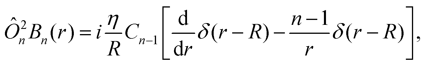 | (8) |
 and η is the force in complex notation η = |f0|e−iarg(f0). The solution is given only by the real part of eqn (8). This equation implies that a Fourier component n in the stream function ψ is caused by a component n − 1 of the force. For example, a force caused by two opposing normal point forces on the surface has only odd components, which leads to only even components in ψ. Every Fourier component, Bn(r), in the stream function ψ is a linear combination of four power laws in
  , where only negative exponents will contribute at r > R (see ESI† for a detailed solution). Outside the particle, at r > R the solution is a linear combination of terms of the form
![[thin space (1/6-em)]](https://www.rsc.org/images/entities/char_2009.gif) lnr, sin(2θ), sin(nθ)/rn, sin(θ)/rn−2 (ignoring phases), where the logarithm is due to a degeneracy for n = 0. The complete solution outside the particles is given by
lnr, sin(2θ), sin(nθ)/rn, sin(θ)/rn−2 (ignoring phases), where the logarithm is due to a degeneracy for n = 0. The complete solution outside the particles is given by | (9) |
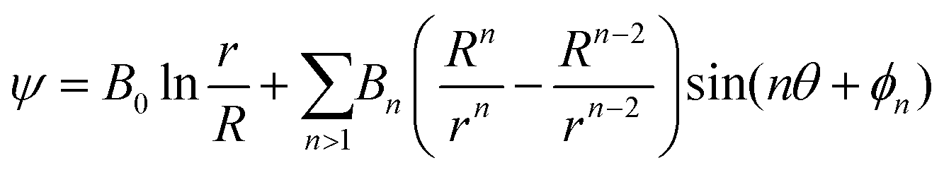 | (10) |
2 Two particle dynamics
This section will focus on a particular example of the flow given by a single force multipole, as given by eqn (9), and the dynamics of two particles interacting by such a flow. We will then discuss the dynamics of two particles interacting by a general solution to eqn (6), with any desired force distribution. We will show that when the particles are oriented, similar particles driven by a pure, even, multipolar term will always collide, the only exceptions being the force monopole and force dipole. For some general force distribution, two particles will always attract in the far-field limit, given that the total force is zero and there is no contribution from a force dipole. If there are no local minima and maxima in the stream function, the particles will also collide. Active particles that do not have a force nor a force dipole are termed neutral swimmers,42,43 and have been shown to have optimal efficiency for spherical particles.44 Biological examples include Volvox45 and Paramecium. Artificial examples could be designed using active Janus particles driven either phoretically10 or by light.112.1 Case study: octopole term
We will consider a force distribution such that only the third harmonic of the force distribution is present. In eqn (3), this corresponds to the forth term, D4 dominating, and the stream function is given by: | (11) |
 | (12) |
 | ||
| Fig. 2 A realization of a particle whose stream function's leading term is 1/r2, which is the octopole term in eqn (3), using point forces. We investigate the interaction between two identical particles with this force distribution, with a fixed orientation. | ||
From this point on, for simplicity, we will focus on one of the terms in eqn (12) and take ψ = Ssin(4θ)/r2 (this can be realized with a force distribution at two different directions, see ESI†). This choice of flow was made for simplicity, but it represents well the general case for the dynamics caused by any single (even) term. Its corresponding flow is displayed in Fig. 3. A system of two identical particles creating such a flow is described by the Hamiltonian in eqn (5).
 | ||
Fig. 3 The vector field generated by a stream function  , where blue corresponds to low strength and red is high. In purple we mark example paths that a particle can take. The straight paths are characterized by a zero Hamiltonian, and alternate being stable or unstable. The leaf-shaped paths are for the non-zero case, alternating a positive and negative Hamiltonian. , where blue corresponds to low strength and red is high. In purple we mark example paths that a particle can take. The straight paths are characterized by a zero Hamiltonian, and alternate being stable or unstable. The leaf-shaped paths are for the non-zero case, alternating a positive and negative Hamiltonian. | ||
In Hamiltonian mechanics, symmetries of the Hamiltonian correspond to conservation laws. In this case, the Hamiltonian is symmetric to translation in time and space. Therefore, the Hamiltonian is conserved as well as, what we term, the “center of activity”, (r1 + r2)/2, which is analogous to the center of mass. It is therefore enough to consider the dynamics of the relative difference between particles d = r1 − r2, which has a 2D phase-space. The paths d can take are displayed in Fig. 3, which are given by r2 ∝ sin(4θ) as a result of the conservation of the Hamiltonian H = ψ(d). It is also straightforward to solve the equations of motion directly, giving
 | (13) |
 which are given by half the period of the harmonic. Also, in general, the radius does not decrease monotonically with time, however it always decreases to zero unless H = 0. The special paths with H = 0 are the only paths that will not necessarily converge to the origin. In principle, they can diverge to infinity, though a divergence is unstable as even a small perturbation to the Hamiltonian will cause the path to be bound. Therefore, every stable solution of the pair leads to a collision. We will now prove that, in the far-field limit, this holds true in general, except for dipolar force terms.
2.2 General dynamics of two particles
Let us consider a case of two identical particles, each creating a stream function ψ that is described by a single (even) multipole term in the far-field limit. We will later consider a dipolar flow which is given by ψ = αlnr + β![[thin space (1/6-em)]](https://www.rsc.org/images/entities/i_char_2009.gif) sin(2θ + ϕ). Any other flow is given by
sin(2θ + ϕ). Any other flow is given by | (14) |
To prove this claim, we will examine the paths that the relative distance between particles, d, takes in its phase-space, whose motion is governed by ψ, ḋ = 2∇⊥ψ(d). The “grad perp” operator, ∇⊥, has an important geometrical interpretation: unlike the gradient, which points to the direction where a scalar function is most increasing, the “grad perp” operator points to the direction perpendicular to that (anti-clockwise) which is also the direction where the function is constant. This interpretation is connected to the fact that H is conserved along paths.
First, we note that the stream function has no local maxima/minima, as a cross section of it at a constant θ gives ψ ∝ r−m, which never has local extrema. Thus, a point path is unstable. This is expected since a stable point would have a negative divergence of the velocity field. Thus, every path curve must be either closed or diverging to infinity. And, since ψ(r → ∞) = 0, every path diverging to infinity has a zero Hamiltonian, and every path with non-zero Hamiltonian is necessarily bound and closed. The different possible path categories are shown in Fig. 4. We will now assess whether or not each is possible.
 | ||
| Fig. 4 The categories of possible paths for the separation between two-active particles, d. If bound, the path either encircles the origin, does not encircle it, or crosses it. If the path diverges, then it either crosses the origin or not. Each path is described by an equation ψ(x,y) = H. In the text we prove which paths are permitted and under what circumstances. | ||
Path a. A closed path that does not contain the origin, such as path a, encircles an area which is a compact subset of the phase-space, where ψ is continuous. Because the stream function is constant along the edge of the region, that is, along a path, there must be a local minimum or maximum inside that region, contradicting our earlier conclusion (this is a higher dimensional case of Rolle's theorem46). This argument, which disallows paths like a, does not hold for the closed paths like d and e because their closed area contains the origin, and so the stream function is not continuous on it.
Paths b and c. Now consider a path that diverges to infinity, like paths b and c. As mentioned, such a path has zero Hamiltonian, so every path that crosses it must also have zero Hamiltonian. Therefore, the curve will split the plane in two—paths on one side of the curve that have a non-zero Hamiltonian cannot cross to the other side. For paths like b, there is a side which does not contain the origin, and so closed paths contained in it must be like path a. Since we showed such paths are not allowed, it then follows that all paths in that side have zero Hamiltonian, and thus ψ = 0. We assume that there cannot be such an area in which the stream function is constant since that corresponds to an area with no flow. That means every path diverging to infinity must cross the origin, That is, it must be similar to path c. In fact, a path similar to path c must exist, because there is some θ0 ∈ [0,2π) such that ψ(r,θ0) = 0 for all r, and so the ray θ = θ0 is a path similar to path c.
Path d. Since a divergent path such as c necessarily exists, every closed path encircling the origin (path d) crosses it. Thus, it also has a zero Hamiltonian. Here, again, the path splits the plane in two and forces paths similar to path a. Therefore, such a path as d cannot exist.
In conclusion, the only possible paths are either closed curves crossing the origin such as path e or divergent curves with a zero Hamiltonian crossing the origin such as path c. However, the side of the divergent path that goes to infinity as time increases is unstable. Consider a small perturbation to the Hamiltonian, H = ε ≠ 0, the particle's trajectory must now be bound. Thus, it is unstable and will turn to path e. And so, every stable path crosses the origin, which corresponds to the particles colliding.
This conclusion only applies to the far-field limit. As the particles get closer, eventually, higher-order terms of the flow will contribute to the dynamics. If the stream function ψ has no minima or maxima, even in close-range, then by the same reasoning as above, the particles will collide because the only allowed paths are still c and e. However, if the stream function has an extremum in close range, then all path types are allowed. Particles will still aggregate up to these short distances.
Let us now consider the different paths that the dipolar terms allow. If the stream function contains a dipolar term of the form sin2θ, then paths that diverge to infinity can have a non-zero Hamiltonian, and so paths like b are allowed. If the stream function contains the termlnr, no paths can diverge to infinity, and so paths like d are allowed, while paths like b and c are not allowed. Examples for both are depicted in Fig. 5. Note that paths like path a are never allowed in the absence of extrema.
 | ||
Fig. 5 Phase space (configurational space) examples where dipole terms are allowed showing paths b and d exist in such cases. In blue,  with H = 1.2 and in red with H = 1.2 and in red  with H = 0.8. These paths are also stable, as a perturbation to the Hamiltonian gives a similarly shaped path. with H = 0.8. These paths are also stable, as a perturbation to the Hamiltonian gives a similarly shaped path. | ||
Lastly, we will address the dynamics when ψ is not even. If the stream function is odd (the far-field limit always has a defined parity), then no Hamiltonian can be constructed. However, it is easy to see that now the relative distance, d, is conserved, while the “center of activity” changes with velocity given by v(d). This results in the pair moving together at a constant velocity, and is true even in close range interaction. In general, if v = vO + vE which are even and odd respectively, then
 | (15) |
3 Many particle dynamics
A system of many particles can no longer be solved analytically. However, for an even stream function it is possible to construct a Hamiltonian as in eqn (5), from which follows the conservation of the center of activity as well as H itself. We integrate over the system's equations of motion using the python library scipy.integrate.DOP853, which is an 8th order Runge–Kutta method. Since the particles are expected to collide, we also add steric interactions to the system, given by Δvsteric = ksteric(lsteric − |rij|)
![[r with combining circumflex]](https://www.rsc.org/images/entities/b_char_0072_0302.gif) ij if |rij| < lsteric and zero otherwise, where rij is the distance from the i-th and j-th particles. The steric interaction gives a strong repelling force when particles overlap. In our simulation we used lsteric = 0.5 and ksteric = 104. The new interactions break the Hamiltonian description, and so H is no longer conserved. However, the center of activity should remain constant as the interaction is still symmetric. In addition, between collisions the Hamiltonian is still conserved (see Fig. 6). The steric interactions are a highly simplified description of the close-range forces between active particles that are not described by Stokes flow.
ij if |rij| < lsteric and zero otherwise, where rij is the distance from the i-th and j-th particles. The steric interaction gives a strong repelling force when particles overlap. In our simulation we used lsteric = 0.5 and ksteric = 104. The new interactions break the Hamiltonian description, and so H is no longer conserved. However, the center of activity should remain constant as the interaction is still symmetric. In addition, between collisions the Hamiltonian is still conserved (see Fig. 6). The steric interactions are a highly simplified description of the close-range forces between active particles that are not described by Stokes flow.
 | ||
| Fig. 6 The Hamiltonian of a 4-particle system during a collision. A swift change in the Hamiltonian is observed at time t = 8.5 when a collision occurs. | ||
We initialize hundreds of randomly positioned particles. Each particle creates the velocity field discussed in Section 3. Namely, we take an octopolar flow with the stream function ψ = sin4θ/r2. Since we have established the similarity of all far-field flows, excluding dipolar flow, as well as flows created by stream functions with no extrema, we can use this simulation to infer the behavior of ensembles interaction via such stream functions. The result of the simulation for different times is displayed in Fig. 1.
Immediately, pairs of particles start attracting and eventually collide. This behavior is a direct result of the two-particle dynamics, because the stream function falls fast with r, ψ ∼ r−2, and so the majority of a particle's motion is determined by its closest neighbor, while the weak effect of other particles forces it to take stable paths only. The colliding particles quickly align at perfect 45° lines, corresponding to the angles where the velocity field is radial only. The stability results from the steric interactions—once the particles collide, the steric force cancels any velocity in the radial direction, and the particles slide on each other until the tangential velocity is also zero. Since the velocity field increases near the particle, the sliding motion is very fast compared to the global dynamics. Thus, a collision is characterized by a swift change to the Hamiltonian since the pair's contribution to H changed from relatively constant (in time) to zero. We clearly see this rapid change in Fig. 6, which shows a simulation for four particles. A collision of two particles is clearly observed by the decrease in the Hamiltonian at t = 8.5. In simulations of hundreds of particles, collisions are too frequent to see the effect clearly.
The two-particle behavior described above repeats on a global scale: all the particles collide into clusters, and all the clusters collide into bigger clusters. This is because, at large distances, a cluster functions as a particle whose strength is the combined strength of its constituents. Therefore, the dynamics of clusters can be described by a Hamiltonian in eqn (5), now with varying strengths. The center of activity is now given by  and is still conserved. In the case of two-cluster dynamics, the vector d = r1 − r2 is sufficient to describe the dynamics, and its equation of motion is ḋ = (S1 + S2)∇⊥ψ(d). Therefore the two-cluster dynamics also lead to a collision, resulting in the clusters mimicking the behavior of the particles. The collisions continue until all the particles form a single stable cluster in the form of an incomplete square lattice, see Fig. 1. This final result can be deduced from the Hamiltonian, since, in each collision, the formed cluster must have zero Hamiltonian (i.e. its self interaction).
The crystallization is thus a general behavior of any ensemble of identical particles that are oriented along the same direction, as long as the two-particle dynamics lead to a collision, in the manner discussed in Section 2.2. Particles will tend to stabilize in incomplete crystal clusters, with an angle approximately given by the lowest power term of the stream function, which is dominant at close-range interactions. More precisely, the stability angles are such that the velocity field at the particles' radius (lsteric/2) at those angles is radial only. Of course, this generalized conclusion is true if the system does not find dynamic stability.
In cases where the stream function is not a pure multipole and possesses extremum points, the dynamics do not necessarily result in the collision of two particles. The particles still draw closer up to distances where the next-order multipole term starts to dominant. Two examples of such cases are given in the ESI.† One still results in crystallization, with particles tending to stay at minimal points of the stream function. The second example is of squirmers. The particles draw closer, but within the aggregate, there are still chaotic dynamics.
4 Conclusions
In this work, we introduced a new method to characterize the flow created by 2D active particles, working directly with a stream function instead of the velocity field. We used this method to investigate the dynamics of a two-particle system, which we then used to infer the behavior of a multi-particle ensemble. We found that in all cases where the stream function does not have a local extremum and does not have a contribution from the monopole or the dipole terms, two particles will always collide. This includes all cases where the flow field is given by a pure even force moment (such as in the far-field limit). Our simulations suggest that many-body systems of such particles aggregate into a cluster. The formed clusters appear to be fractal-like and are somewhat reminiscent of diffusion-limited aggregation47 but with two differences—(1) particle motion is driven by active flows, not diffusion. In fact, the only random component is in the initial positions of the particles. (2) There is short-range repulsion between particles, not attraction. Particles stick together due to the balance between steric interactions and active flows.The steps we took in this paper are not limited to a simple description of 2D fluid dynamics, but can be generalized to other effective 2D fluids with more complex flow equations. Such systems are commonly encountered in biological membranes,6,7,48,49 or in experimental systems when particles sediment close to the bottom or float to the interface.11,50–52 Such cases are associated with Green's functions that differ from eqn (2) and flow equations that differ from eqn (6). Solutions to their flow equations will produce all the force multipoles of those systems.
In addition, the arguments and results laid out in Section 2.2, regarding possible paths that two particles can take, are also relevant to these more complex systems, in describing oriented particles. The requirements for particle dynamics to result in a collision are: (a) the stream function has no extrema, e.g. by the Hessian test (and twice-differentiability everywhere except the origin). (b) ψ(r → ∞) = 0, and (c) there is at least one path diverging to infinity.
For instance, in a membrane, at small distances, the fluid is conserved in the membrane, and the flow created by an active protein is given by the dipole terms in eqn (9). At large distances, momentum is exchanged with the outer three-dimensional fluid.48,53 An active particle in a membrane at large distances creates a flow with a stream function that dies out at infinity, as  .7 The ray θ = 0 is a path diverging to infinity. The Hessian is negative, detH(ψ) = −2S(5 + 3cos22θ)/r6 < 0. Thus, two oriented active proteins interacting via this stream function are bound to aggregate.
We have pointed out a connection between two-particle dynamics and multi-particle dynamics. It is tempting to say that as long as ψ ∼ r−1 or lower, such that two particles must collide (per our discussion in Section 2.2), then larger systems will exhibit the same dynamics because the interactions are dominated by the nearest neighbors. However, it is unclear if this assessment is necessarily correct. Based on our findings, we hypothesize that such a conclusion is correct, but it remains for future work to assess its validity.
Our analysis was restricted to cases where the particles are all oriented along the same direction. Such a setting can arise either in a flocking mode,54 in which case particles can rotate but are more likely to rotate together, or when the particles are all oriented due to an external field.55 In the latter case, the point particles we consider do not experience a torque, but particles with a finite size will experience a torque. From Faxén's second law56 in 2D we expect T ∝ a2(∇ × v). When this torque is reflected to other particles, it will induce a higher-order flow decaying as 1/r2 times the original flow. In such cases, we still expect condensation up to shorter distances where the torque may become significant. In future work, we hope to generalize our results to cases where the particles are free to rotate, in which case a Hamiltonian description is challenging.
We have focused on interactions that lead to collisions between two particles—those of pure multipolar flows and cases where there are no extremum points in the stream function. In other types of dynamics, particles attract up to a certain distance, but there is no static final state. Ensembles with such interactions can have chaotic dynamics, but also global structures and order, as mentioned in the ESI.† These systems require closer examination.
We have limited our discussion to far-field hydrodynamic interactions in the low Reynolds limit. However, it is clear that in close range, the interaction of the particles can be influenced by other effects. For Instance, Yoshinaga and Liverpool57 showed the importance of lubrication forces in dense interaction between active swimmers, which may affect the crystallization and stability of a many-particle ensembles. Similar effects are expected to change the final state of our system, but in principle, the characteristics of the far-range interactions should remain the same, meaning the particles are still expected to aggregate into large clusters.
Conflicts of interest
There are no conflicts to declare.Acknowledgements
This research was supported by the Israel Science Foundation (grant No. 1752/20).Notes and references
- E. Lauga, W. R. DiLuzio, G. M. Whitesides and H. A. Stone, Swimming in circles: motion of bacteria near solid boundaries, Biophys. J., 2006, 90(2), 400–412 CrossRef CAS PubMed.
- E. Lushi, H. Wioland and R. E. Goldstein, Fluid flows created by swimming bacteria drive self-organization in confined suspensions, Proc. Natl. Acad. Sci. U. S. A., 2014, 111(27), 9733–9738 CrossRef CAS PubMed.
- C. J. Miles, A. A. Evans, M. J. Shelley and S. E. Spagnolie, Active matter invasion of a viscous fluid: Unstable sheets and a no-flow theorem, Phys. Rev. Lett., 2019, 122(9), 098002 CrossRef CAS PubMed.
- J. D. Robertson, Membrane structure, J. Cell Biol., 1981, 91(3), 189 CrossRef CAS PubMed.
- P. Lenz, J. F. Joanny, F. Jülicher and J. Prost, Membranes with rotating motors, Phys. Rev. Lett., 2003, 91(10), 108104 CrossRef PubMed.
- N. Oppenheimer, D. B. Stein and M. J. Shelley, Rotating Membrane Inclusions Crystallize Through Hydrodynamic and Steric Interactions, Phys. Rev. Lett., 2019, 10(123), 148101 CrossRef PubMed.
- H. Manikantan, Tunable collective dynamics of active inclusions in viscous membranes, Phys. Rev. Lett., 2020, 125(26), 268101 CrossRef CAS PubMed.
- J. R. Howse, R. A. Jones, A. J. Ryan, T. Gough, R. Vafabakhsh and R. Golestanian, Self-motile colloidal particles: from directed propulsion to random walk, Phys. Rev. Lett., 2007, 99(4), 048102 CrossRef PubMed.
- H. R. Vutukuri, M. Lisicki, E. Lauga and J. Vermant, Light-switchable propulsion of active particles with reversible interactions, Nat. Commun., 2020, 11(1), 2628 CrossRef CAS PubMed.
- J. Palacci, S. Sacanna, S. H. Kim, G. R. Yi, D. J. Pine and P. M. Chaikin, Light-activated self-propelled colloids. Philosophical Transactions of the Royal Society A: Mathematical, Phys. Eng. Sci., 2014, 372(2029), 20130372 Search PubMed.
- M. Y. Ben Zion, Y. Caba, A. Modin and P. M. Chaikin, Cooperation in a fluid swarm of fuel-free micro-swimmers, Nat. Commun., 2022, 13(1), 184 CrossRef CAS PubMed.
- A. Modin, M. Y. Ben Zion and P. M. Chaikin, Hydrodynamic spin-orbit coupling in asynchronous optically driven micro-rotors, Nat. Commun., 2023, 14(1), 4114 CrossRef CAS PubMed.
- R. Dreyfus, J. Baudry, M. L. Roper, M. Fermigier, H. A. Stone and J. Bibette, Microscopic artificial swimmers, Nature, 2005, 437(7060), 862–865 CrossRef CAS PubMed.
- I. S. Aranson, Active colloids, Phys.-Usp., 2013, 56(1), 79 CrossRef CAS.
- M. M. Genkin, A. Sokolov, O. D. Lavrentovich and I. S. Aranson, Topological defects in a living nematic ensnare swimming bacteria, Phys. Rev. X, 2017, 7(1), 011029 Search PubMed.
- N. Yoshinaga and T. B. Liverpool, Hydrodynamic interactions in dense active suspensions: From polar order to dynamical clusters, Phys. Rev. E, 2017, 96(2), 020603 CrossRef PubMed.
- M. C. Marchetti, J. F. Joanny, S. Ramaswamy, T. B. Liverpool, J. Prost and M. Rao, et al., Hydrodynamics of soft active matter, Rev. Mod. Phys., 2013, 85(3), 1143 CrossRef CAS.
- D. Saintillan and M. J. Shelley, Active suspensions and their nonlinear models, C. R. Phys., 2013, 14(6), 497–517 CrossRef CAS.
- R. Singh and R. Adhikari, Universal hydrodynamic mechanisms for crystallization in active colloidal suspensions, Phys. Rev. Lett., 2016, 117(22), 228002 CrossRef PubMed.
- B. Rallabandi, F. Yang and H. A. Stone, Motion of hydrodynamically interacting active particles, arXiv, 2019, preprint, arXiv:190104311 Search PubMed.
- E. Lushi and P. M. Vlahovska, Periodic and Chaotic Orbits of Plane-Confined Micro-rotors in Creeping Flows, J. Nonlinear Sci., 2015, 10(25), 1111–1123 CrossRef.
- K. Yeo, E. Lushi and P. M. Vlahovska, Collective dynamics in a binary mixture of hydrodynamically coupled microrotors, Phys. Rev. Lett., 2015, 114(18), 188301 CrossRef PubMed.
- R. Samanta and N. Oppenheimer, Vortex flows and streamline topology in curved biological membranes, Phys. Fluids, 2021, 33, 5 Search PubMed.
- N. Oppenheimer, D. B. Stein, M. Y. B. Zion and M. J. Shelley, Hyperuniformity and phase enrichment in vortex and rotor assemblies, Nat. Commun., 2022, 13(1), 804 CrossRef CAS PubMed.
- J. De Graaf and J. Stenhammar, Lattice-Boltzmann simulations of microswimmer-tracer interactions, Phys. Rev. E, 2017, 95(2), 023302 CrossRef PubMed.
- Y. Shoham and N. Oppenheimer, Hamiltonian Dynamics and Structural States of Two-Dimensional Active Particles, Phys. Rev. Lett., 2023, 131(17), 178301 CrossRef CAS PubMed.
- Ž. Kos and M. Ravnik, Elementary flow field profiles of micro-swimmers in weakly anisotropic nematic fluids: Stokeslet, stresslet, rotlet and source flows, Fluids, 2018, 3(1), 15 CrossRef.
- E. Lauga, T. N. Dang and T. Ishikawa, Zigzag instability of biased pusher swimmers, Europhys. Lett., 2021, 133(4), 44002 CrossRef CAS.
- S. Kim and S. J. Karrila, Microhydrodynamics: principles and selected applications, Courier Corporation, 2013 Search PubMed.
- S. E. Spagnolie and E. Lauga, Hydrodynamics of self-propulsion near a boundary: predictions and accuracy of far-field approximations, J. Fluid Mech., 2012, 700, 105–147 CrossRef.
- M. Lisicki, Four approaches to hydrodynamic Green's functions-the Oseen tensors, arXiv, 2013, preprint, arXiv:13126231, DOI: 10.48550/arXiv.1312.6231 Search PubMed.
- L. Onsager, Statistical hydrodynamics, Il Nuovo Cimento, 1949, 6(Suppl 2), 279–287 CrossRef CAS.
- P. K. Newton and M. Platzer, N-Vortex Problem: Analytical Techniques, Appl. Mech. Rev., 2002, 55(1), B15–B16 CrossRef.
- A. Zöttl and H. Stark, Nonlinear dynamics of a microswimmer in Poiseuille flow, Phys. Rev. Lett., 2012, 108(21), 218104 CrossRef PubMed.
- R. Chajwa, N. Menon and S. Ramaswamy, Kepler orbits in pairs of disks settling in a viscous fluid, Phys. Rev. Lett., 2019, 122(22), 224501 CrossRef CAS PubMed.
- P. Lenz, J. F. Joanny, F. Jülicher and J. Prost, Membranes with rotating motors: Microvortex assemblies, Eur. Phys. J. E: Soft Matter Biol. Phys., 2004, 13, 379–390 CrossRef CAS PubMed.
- A. Bolitho and R. Adhikari, Overdamped Lattice Dynamics of Sedimenting Active Cosserat Crystals, arXiv, 2022, preprint, arXiv:220206102 Search PubMed.
- D. G. Crowdy and Y. Or, Two-dimensional point singularity model of a low-Reynolds-number swimmer near a wall, Phys. Rev. E: Stat., Nonlinear, Soft Matter Phys., 2010, 81(3), 036313 CrossRef PubMed.
- D. G. Crowdy and A. M. Davis, Stokes flow singularities in a two-dimensional channel: a novel transform approach with application to microswimming, Proc. R. Soc. A, 2013, 469(2157), 20130198 CrossRef PubMed.
- M. J. Lighthill, On the squirming motion of nearly spherical deformable bodies through liquids at very small Reynolds numbers, Commun. Pure Appl. Math., 1952, 5(2), 109–118 CrossRef.
- J. R. Blake, A spherical envelope approach to ciliary propulsion, J. Fluid Mech., 1971, 46(1), 199–208 CrossRef.
- S. Ghose and R. Adhikari, Irreducible representations of oscillatory and swirling flows in active soft matter, Phys. Rev. Lett., 2014, 112(11), 118102 CrossRef PubMed.
- A. Andersen, N. Wadhwa and T. Kiørboe, Quiet swimming at low Reynolds number, Phys. Rev. E: Stat., Nonlinear, Soft Matter Phys., 2015, 91(4), 042712 CrossRef PubMed.
- A. Daddi-Moussa-Ider, B. Nasouri, A. Vilfan and R. Golestanian, Optimal swimmers can be pullers, pushers or neutral depending on the shape, J. Fluid Mech., 2021, 922, R5 CrossRef CAS.
- K. Drescher, K. C. Leptos, I. Tuval, T. Ishikawa, T. J. Pedley and R. E. Goldstein, Dancing volvox: hydrodynamic bound states of swimming algae, Phys. Rev. Lett., 2009, 102(16), 168101 CrossRef PubMed.
- M. Furi and M. Martelli, A multidimensional version of Rolle's theorem, Am. Math. Mon., 1995, 102(3), 243–249 CrossRef.
- T. A. Witten Jr and L. M. Sander, Diffusion-limited aggregation, a kinetic critical phenomenon, Phys. Rev. Lett., 1981, 47(19), 1400 CrossRef.
- P. Saffman and M. Delbrück, Brownian motion in biological membranes, Proc. Natl. Acad. Sci. U. S. A., 1975, 72(8), 3111–3113 CrossRef CAS PubMed.
- Y. Hosaka, K. Yasuda, R. Okamoto and S. Komura, Lateral diffusion induced by active proteins in a biomembrane, Phys. Rev. E, 2017, 95(5), 052407 CrossRef PubMed.
- D. Lopez and E. Lauga, Dynamics of swimming bacteria at complex interfaces, Phys. Fluids, 2014, 26(7), 071902 CrossRef.
- A. C. H. Tsang and E. Kanso, Flagella-induced transitions in the collective behavior of confined microswimmers, Phys. Rev. E: Stat., Nonlinear, Soft Matter Phys., 2014, 90(2), 021001 CrossRef PubMed.
- H. Wioland, F. G. Woodhouse, J. Dunkel, J. O. Kessler and R. E. Goldstein, Confinement stabilizes a bacterial suspension into a spiral vortex, Phys. Rev. Lett., 2013, 110(26), 268102 CrossRef PubMed.
- N. Oppenheimer and H. Diamant, Correlated diffusion of membrane proteins and their effect on membrane viscosity, Biophys. J., 2009, 96(8), 3041–3049 CrossRef CAS PubMed.
- N. C. Darnton, L. Turner, S. Rojevsky and H. C. Berg, Dynamics of bacterial swarming, Biophys. J., 2010, 98(10), 2082–2090 CrossRef CAS PubMed.
- G. Junot, M. De Corato and P. Tierno, Large scale zigzag pattern emerging from circulating active shakers, Phys. Rev. Lett., 2023, 131(6), 068301 CrossRef CAS PubMed.
- H. Faxén, Der Widerstand gegen die Bewegung einer starren Kugel in einer zähen Flüssigkeit, die zwischen zwei parallelen ebenen Wänden eingeschlossen ist, Ann. Phys., 1922, 373(10), 89–119 CrossRef.
- N. Yoshinaga and T. B. Liverpool, From hydrodynamic lubrication to many-body interactions in dense suspensions of active swimmers, Eur. Phys. J. E: Soft Matter Biol. Phys., 2018, 41, 1–22 CrossRef CAS PubMed.
Footnote |
| † Electronic supplementary information (ESI) available: Including full derivation of the stream function, constraints on the force distribution, instructions on how to construct multiples using point forces, and examples of cases where the flow has extremum points. See DOI: https://doi.org/10.1039/d3sm01670f |
| This journal is © The Royal Society of Chemistry 2024 |