DOI:
10.1039/D3SM01480K
(Paper)
Soft Matter, 2024,
20, 3007-3020
Motion of microswimmers in cylindrical microchannels†
Received
2nd November 2023
, Accepted 7th March 2024
First published on 8th March 2024
Abstract
Biological and artificial microswimmers often have to propel through a variety of environments, ranging from heterogeneous suspending media to strong geometrical confinement. Under confinement, local flow fields generated by microswimmers, and steric and hydrodynamic interactions with their environment determine the locomotion. We propose a squirmer-like model to describe the motion of microswimmers in cylindrical microchannels, where propulsion is generated by a fixed surface slip velocity. The model is studied using an approximate analytical solution for cylindrical swimmer shapes, and by numerical hydrodynamics simulations for spherical and spheroidal shapes. For the numerical simulations, we employ the dissipative particle dynamics method for modelling fluid flow. Both the analytical model and simulations show that the propulsion force increases with increasing confinement. However, the swimming velocity under confinement remains lower than the swimmer speed without confinement for all investigated conditions. In simulations, different swimming modes (i.e. pusher, neutral, puller) are investigated, and found to play a significant role in the generation of propulsion force when a swimmer approaches a dead end of a capillary tube. Propulsion generation in confined systems is local, such that the generated flow field generally vanishes beyond the characteristic size of the swimmer. These results contribute to a better understanding of microswimmer force generation and propulsion under strong confinement, including the motion in porous media and in narrow channels.
1 Introduction
In their natural habitat, biological microswimmers (e.g. E. coli, Paramecium) are subject to a multitude of different environments, ranging from unconfined liquid media to porous-like surroundings within the soil or a biofilm.1,2 Properties of these media can be very diverse, and include fluid viscosity varying over several orders of magnitude,3,4 viscoelasticity in complex fluidic environments,5,6 and various degrees of hard and soft confinements.7–9 In such environments, microswimmers are subject to intricate steric and hydrodynamic interactions,10,11 which they have to cope with and be able to employ for their efficient locomotion and navigation. Furthermore, understanding microswimmer propulsion in complex environments is relevant for the development of microscopic artificial motile systems capable of performing specific tasks.12,13
Most studies of locomotion under confinement have focused on microswimmer-wall interactions.2,14 For example, microswimmers are subject to wall accumulation, which is due to their slow re-orientation (e.g. governed by rotational diffusion) after they hit a wall as well as hydrodynamic interactions.15–17 The accumulation is even more enhanced in places with a non-zero wall curvature,18–20 and this effect can lead to a persistent microswimmer motion along the surface.21,22 Studies of microswimmer propulsion under strong confinements are still rather scarce due to difficulties in experimental observations or numerical modeling. For instance, E. coli in porous media exhibits hopping and trapping behavior,7 in contrast to the run-and-tumble motion within unconfined fluidic environments.23 Furthermore, trypanosomes (parasites causing sleeping sickness) can survive in and navigate through very different environments, including blood and several solid-like tissues.6,24 An investigation of trypanosome locomotion through a maze of obstacles within a microfluidic device suggested that these parasites can sometimes move more efficiently through crowded environments.25 Nevertheless, the majority of experimental and theoretical studies report a reduction in microswimmer speed under confinement in comparison with that within unconfined fluid conditions.7,26–28
Another interesting example is the motion of microswimmers under soft deformable confinements represented by a lipid membrane and vesicles.8,9,29,30 This active system shows a variety of dynamic non-equilibrium vesicle shapes, including prolate geometries and structures with multiple tether-like protrusions generated by the encapsulated swimmers. Within the tethers, the swimmers are tightly wrapped by the membrane; however, they are still able to propel and exert forces on the membrane to further extend the tethers. E. coli bacteria were found not only to pull relatively long tethers, but also to transport the vesicle with a non-zero velocity despite the tight wrapping by the vesicle membrane.29
The examples above raise a number of scientific questions related to microswimmer propulsion under confinement. How can microswimmers propel and navigate through very confined environments? Do they employ the physical mechanisms and strategies similar to those when propelling under unconfined conditions? Does the local flow field generated by microswimmers play an essential role in their propulsion under strong confinements? Can they propel faster within confined environments in comparison to that within unconfined surroundings?
To address some of these questions, we investigate squirmer behavior in cylindrical microchannels. In particular, we develop a theoretical model of swimmer motion within a cylindrical capillary tube, which predicts its propulsion force and velocity as a function of confinement and its swimming strength. Furthermore, we perform simulations of microswimmer locomotion in a tube using a squirmer model.31–33 In both the theoretical model and simulations, periodic boundary conditions along the capillary axis as well as an impenetrable wall at the ends of the tube, representing a dead end, are considered. Simulation results confirm that the approximation of the analytical model properly captures the qualitative behavior of a squirmer inside a cylindrical microchannel. In the squirmer model with fixed surface slip velocity, the propulsion force increases with increasing confinement, while the swimming velocity always remains smaller than the swimmer speed for unconfined conditions, suggesting that the drag on the swimmer increases faster than the propulsion force with confinement. The model shows that a swimmer is expected to be able to move even under very strong confinements, though an increasing power with increasing confinement is required. The analytical model does not consider details of the local flow field generated by the swimmer, while in simulations, the squirmer model allows the imposition of different local flow fields, corresponding to pusher, neutral, and puller swimmers.33 The swimming velocities in long channels only differ slightly among these three swimming modes. However, the propulsion forces near dead ends of the tube differ substantially. These results help us better understand swimming behavior under confinement, including tether pulling from fluid vesicles by encapsulated microswimmers.8,9,29,30
The article is organized as follows. Section 2 provides all necessary details about the employed methods and models. Section 3 presents the approximate analytical model of swimmer propulsion in a capillary tube. The corresponding simulations using the squirmer model are presented in Section 4, and compared with the analytical model. We discuss the results and shortly conclude in Section 5.
2 Methods and models
2.1 Swimmer model: squirmers
We represent the swimmer as a squirmer, a geometric body with a prescribed slip velocity on its surface. Geometry of the squirmer body and its surface velocity field are axisymmetric. Three squirmer shapes, spherical, spheroidal and cylindrical are considered.
Propulsion of the spherical squirmer is implemented according to the classical squirmer model33 as
| | usurf = (B1![[thin space (1/6-em)]](https://www.rsc.org/images/entities/char_2009.gif) sin(θ) + B2sin(θ)cos(θ))tθ, sin(θ) + B2sin(θ)cos(θ))tθ, | (1) |
where in spherical coordinates
θ is the angle between the orientation of the squirmer and the vector from the center of mass to a point on the surface, and
tθ is the tangent vector in
θ-direction. The coefficient
B1 defines propulsion strength of the swimmer and
B2 introduces fore-and-aft asymmetry into the slip-velocity field. A spherical squirmer swims in bulk fluid with a velocity

. We use the ratio
β =
B2/
B1 to capture the modality. For
β > 0 the squirmer is called a puller, for
β = 0 it is neutral and for
β < 0 it is a pusher.
The spheroidal squirmer is a generalization of the spherical shape, and describes a class of prolate-shaped squirmers. Adaptation of eqn (1) to a spheroidal shape is described in Appendix A. The speed of a spheroidal squirmer increases from  for a spherical squirmer to v0 = B1 as a function of increasing aspect ratio of the spheroidal shape.34
For the cylindrical squirmer, we consider a shape with a radius rcyl and a length Lcyl (see Fig. 1). Squirmer propulsion is facilitated by a polar surface slip velocity (usurf = ucylez for r = rcyl) of constant magnitude ucyl on its jacket from front to back. No-slip boundary conditions are assumed at the front and rear surfaces of the cylinder. This is motivated by neutral squirmers, whose polar surface slip velocity is also axisymmetric, has a maximum at the equator, and vanishes at the poles. Furthermore, this model facilitates the construction of an approximate analytical solution of the squirmer motion inside cylindrical microchannels.
 |
| | Fig. 1 Schematic of a cylindrical swimmer in a periodic cylindrical capillary tube. The swimmer has a radius rcyl and a length Lcyl, while the capillary is characterized by a radius Rcap and a length Lcap. p1 and p2 denote pressures at the back and the front of the swimmer, respectively. A free swimmer moves with a velocity vsq. The swimmer's center of mass (the black point at z = 0) can also be held by a spring (red line), in order to measure its propulsion force. Boundary conditions of the flow are given by the slip velocity ucyl at the swimmer surface and the no-slip condition at the capillary wall. | |
2.2 Modeling fluid flow
To model fluid flow in simulations, we employ the dissipative particle dynamics (DPD) method,35–37 a mesoscopic simulation technique. In DPD, the fluid is represented by a collection of particles which correspond to small fluid volumes and interact through three types of pairwise forces. Thus, the force on fluid particle i is given by| | 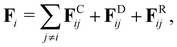 | (2) |
where the sum runs over particles j that are neighbors of the particle i, and includes conservative (FC), dissipative (FD), and random (FR) forces. The conservative force FCij = aijωC(rij)![[r with combining circumflex]](https://www.rsc.org/images/entities/b_char_0072_0302.gif) ij supplies a soft repulsion between DPD particles with a strength coefficient aij, where rij = ri − rj, rij = |rij|, ij = rij/rij. We introduce a weight function ω of the general form
ij supplies a soft repulsion between DPD particles with a strength coefficient aij, where rij = ri − rj, rij = |rij|, ij = rij/rij. We introduce a weight function ω of the general form| | 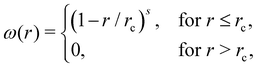 | (3) |
where rc is the cutoff radius beyond which all interactions vanish, and s is an exponent to modify the weight function. The other two forces are FDij = −γωD(rij)(ij·vij)ij and  where γ and σ are the force strength coefficients, vij = vi − vj, ξij = ξji is a Gaussian random variable with zero mean and unit variance, and Δt is the time step. The fluctuation–dissipation theorem relates these weight functions and the force coefficients as36
| | | ωD(r) = [ωR(r)]2 = ω(r), σ2 = 2γkBT. | (4) |
Thus, the pair of dissipative and random forces corresponds to a thermostat which maintains a constant temperature T in the simulated fluid.
2.3 Numerical implementation of the spherical and spheroidal squirmer
In simulations, the squirmer is modeled by a triangulated network of particles which are placed homogeneously on the swimmer surface. In order to maintain a nearly rigid shape of the squirmer, the triangulated network of particles incorporates shear elasticity, bending rigidity, and constraints for the surface area and enclosed volume.38,39 Bonds between neighboring vertices of the network supply shear elasticity and are described by the potential Ubond = UWLC + UPOW38 with| |  | (5) |
where x = l/lm ∈ (0,1), l is the spring length, lm the maximum spring extension, p the persistence length, and kp the repulsive force coefficient. The bending resistance is implemented through the discretization of the Helfrich bending energy40,41 as| |  | (6) |
where κ is the bending rigidity,  is the discretized mean curvature at vertex i, ni is the unit normal at the membrane vertex i,
  is the area corresponding to vertex i (the area of the dual cell), j(i) corresponds to all vertices linked to vertex i, and σij = rij(cotθ1 + cotθ2)/2 is the length of the bond in the dual lattice, where θ1 and θ2 are the angles at the two vertices opposite to the edge ij in the dihedral. Finally, Hi0 is the spontaneous curvature at vertex i, which can be used to implement shapes with non-constant local curvatures (e.g. spheroidal surfaces).
The area and volume conservation constraints are introduced through the potentials38
| |  | (7) |
| |  | (8) |
where
A is the instantaneous area of the membrane,
Atot0 the targeted global area,
Am the area of the
m-th triangle,
Am0 the targeted area of the
m-th triangle determined by the triangular mesh on the squirmer surface,
V the instantaneous membrane volume, and
Vtot0 the targeted volume. Furthermore,
ka,
kd, and
kv are the global area, local area and volume constraint coefficients, respectively.
Nt is the number of triangles on the triangulated surface.
The swimmer is embedded in a DPD fluid. DPD particles are also placed inside the swimmer. The swimmer surface, described by a membrane, is impenetrable for DPD fluid particles and separates them into an inside and outside volume. The separation of DPD fluid particles by the squirmer membrane is necessary for a proper imposition of slip boundary conditions at the squirmer surface. Note that the dissipative and random forces between fluid particles inside and outside the membrane are turned off, while the conservative force is used to keep homogeneous fluid pressure across the membrane.38 To prevent fluid particles from crossing the membrane, their reflection from both sides of the membrane is implemented following a rule,42 in which particle positions are updated according to specular reflection, while particle velocities follow the bounce-back reflection.
To enforce the slip velocity at the swimmer surface, dissipative interaction between swimmer particles and those of outer fluid is modified as
| |  | (9) |
where
uisurf is the slip velocity at the position of swimmer particle
i, while
j represents an outer-fluid particle. There also exist other approaches that implement swimmer motion in a DPD fluid.
43–45
2.4 Model of solid walls
Solid walls are represented by frozen DPD particles which have the same number density and interactions as fluid particles. The frozen wall particles facilitate no-slip boundary conditions (BCs) at the walls through dissipative interactions with fluid particles. To prevent fluid particles from penetrating the walls, reflective surfaces are added at the fluid–solid interface, where bounce-back reflection of fluid particles is performed.42 Note that the bounce-back reflection also contributes to the enforcement of no-slip BCs at the walls.
2.5 Simulation parameters
In most simulations, the swimmer has a spherical shape with a radius rsq = 5rc, and is represented by the squirmer model with N = 3000 discretization particles on its surface. To maintain a non-deformable spherical geometry, the targeted membrane area Atot0 is set 5% smaller than 4πrsq2 and the targeted volume Vtot0 5% larger than 4πrsq3/3, such that the surface is under considerable tension. The confinement is modeled by a capillary tube with a radius Rcap using either periodic BCs in the z direction or solid-wall BCs at both ends of the tube. To constrain the swimmer position at the capillary center and its swimming orientation along the z axis, two springs are attached to the front and rear portions of the swimmer, represented by about 300 surface particles with maximum and minimum z coordinates, respectively. Equilibrium position of these springs is set to (0, 0, *), such that the springs control the swimmer position and orientation only in the x and y directions, while the motion along the z direction remains unaffected. In addition to spherically-shaped squirmers, a number of simulations are also performed for a prolate spheroid (N = 1038 particles) with semi-minor axes bx = by = 3rc and a semi-major axis bz = 6rc.
The fluid is modelled by a collection of DPD particles with a number density n = 5/rc3 (rc = 1.0 is selected in simulations). The DPD force coefficients for interactions between fluid particles are given by a = 80kBT/rc,  s = 1 for ωC and s = 0.1 for ωD and ωR, where m = 1 is the particle mass and kBT = 1 is the unit of energy. This results in a fluid dynamic viscosity of
  which is computed in a separate simulation using the reverse Poiseuille flow approach.46,47 Coupling between the spherical squirmer and fluid particles assumes asf = 0 and
 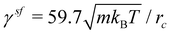 with rsfc = 0.8rc. The value of γsf is computed such that the imposed slip BCs at the squirmer surface are obtained.38 For the spheroidal swimmer,
  because the surface density of squirmer particles is different from that for the spherical swimmer. For simulations with a finer fluid resolution, the density is set to n = 20/rc3, while the cutoff radius is
  to reduce the overall computational cost. In this case, the dynamic viscosity becomes
 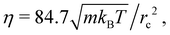 which is close to that in simulations with n = 5/rc3. The time step is
  and the center of mass of the squirmer is sampled every 100 time steps. The velocity is computed using the distance that the swimmer covers within 800 time steps. Error bars represent the standard deviation of these samples.
3 Approximate analytical approach for cylindrical squirmers in microchannels
We first derive an approximate analytic description for a cylindrical squirmer in confinement, sketched in Fig. 1. The confinement is represented by a cylindrical capillary tube with a radius Rcap and a length Lcap, which can either be closed at both ends or have open ends connecting two fluid reservoirs. The latter case is approximated by a capillary tube with periodic BCs along the tube axis. The surface of the capillary tube is subject to no-slip BCs for fluid flow. p1 and p2 correspond to fluid pressures at the back and front ends of the swimmer, respectively. The swimmer axis is assumed to always be parallel to the tube axis and at the centerline of the capillary. We are interested in the velocity vsq of the swimmer, when its propulsion force is balanced by the drag due to surrounding fluid flow. Furthermore, to measure the propulsion force of the swimmer, its center of mass can be pinned by a harmonic spring (see Fig. 1), such that the retaining force of the spring equals the propulsion force of the swimmer. Since we are not able to construct a full analytic solution, an approximate model with several simplifications is considered. In fact, the design of the cylindrical squirmer is chosen such that an approximation for swimming in a narrow cylindrical tube is plausible, at least for swimmers with a large aspect ratio, i.e. Lcyl ≫ rcyl. We neglect the effect of local fluid flow near the back and front ends of the cylinder on the propulsion, i.e., we assume that fluid radial velocity ur is zero everywhere, and consider only fluid flow through a cross-section of the tube. Under the assumption that the microswimmer moves at low Reynolds numbers, fluid flow in this system can be described by the incompressible Stokes equation48η∇2u = ∇p, where η is the dynamic viscosity. In cylindrical coordinates, the general solution of this equation for fluid flow through a cross-section (ur = 0) is given by| |  | (10) |
where c1 and c2 are constants that need to be determined. Explicit expressions for the parameters (e.g. c1 and c2) of the approximate analytical model are given in Appendix B for different conditions. Note that the employed Stokes equation with ur = 0 can also be derived from approximations used in the lubrication theory, so that our assumptions remain valid in the limit of vanishing gap size or when rcyl → Rcap.
3.1 Squirmer in a periodic capillary tube
When the swimmer's center of mass is pinned by a spring, vsq = 0 at steady state and the propulsion force of the swimmer can be measured. The cross-sectional flow profiles can then be derived (i) through the gap between the swimmer and the capillary tube, and (ii) through the tube away from the swimmer. The pressure gradient along the gap is given by ∇pgap = (p2 − p1)/Lcyl = Δp/Lcyl, while the pressure gradient along the swimmer-free section of the capillary is ∇pcap = (p1 − p2)/(Lcap − Lcyl) = −Δp/(Lcap − Lcyl) due to periodic BCs along the tube axis. Then, the corresponding flow profiles are| | 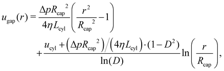 | (11) |
| |  | (12) |
where D = rcyl/Rcap is the confinement. Here, we used BCs at the capillary surface with u(Rcap) = 0 and at the lateral surface of the swimmer with ugap(rcyl) = ucyl. To determine the pressure drop Δp, we use mass conservation which requires the volumetric flow rate through the gap to be equal to the flow rate through the swimmer-free section of the tube. An integral form of mass conservation reads  with ϕ denoting the polar angle. This allows us to compute Δp and fully determine the flow profiles above.
To calculate the propulsion force Fcyl, the fluid stress tensor σ has to be integrated over the microswimmer surface S, i.e. with surface normal n. In cylindrical coordinates with the assumption that ur = uϕ = 0, the stress tensor becomes
| | 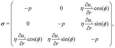 | (13) |
where
p is the hydrostatic pressure. Integration of fluid stresses over the cylindrical surface leads to
| |  | (14) |
Insertion of the solution
ugap(
r) from
eqn (11) results in the propulsion force
| |  | (15) |
As the pressure drop Δ
p is proportional to 1/
Rcap2, the propulsion force in
eqn (15) becomes a function of the confinement
D =
rcyl/
Rcap. The force
Fcyl is displayed in
Fig. 2(a) and (b) for different swimmer and capillary tube lengths. It increases with increasing confinement, and diverges as
D → 1. Note that here our model does not assume any limit on the generated propulsion force (see a discussion in Section 3.2), while forces generated by realistic microswimmers would clearly have a finite upper bound. In the limit of
D → 0, the propulsion force vanishes, suggesting that the swimmer can move without any force generation in an unconfined situation. This is an artifact of model assumptions, where the shear rate

at the cylinder jacket vanishes as
Rcap → ∞ (or
D → 0), so that the shear stress on the cylinder also disappears.
 |
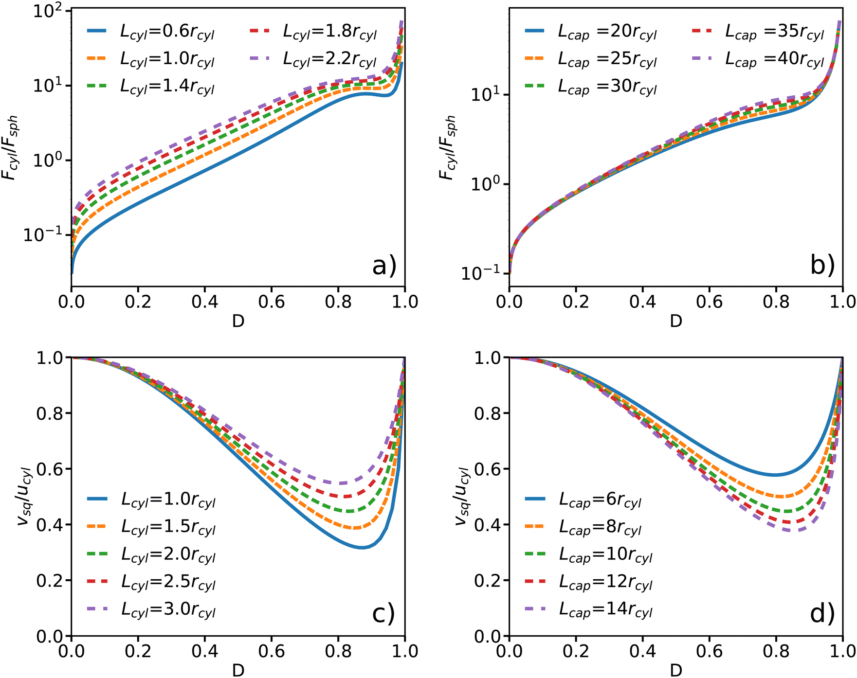
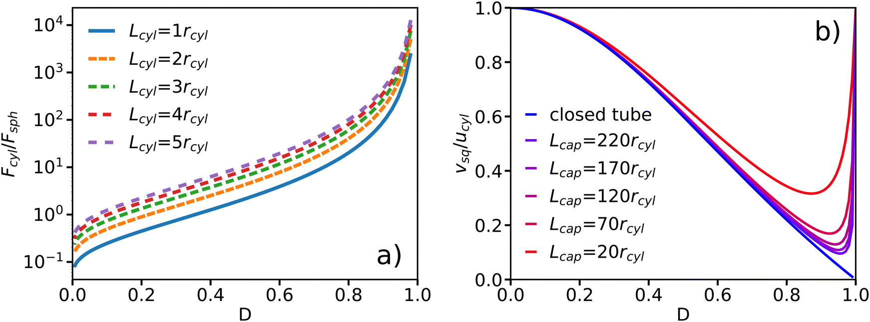
| | Fig. 2 Approximate analytical model for a cylindrical swimmer in a periodic capillary tube. (a) and (b) Propulsion force Fcyl of a spring-pinned swimmer as a function of confinement D for (a) various swimmer lengths with Lcap = 60rcyl and (b) different capillary lengths with Lcyl = 2rcyl. The confinement D = rcyl/Rcap is varied by changing Rcap and the force is normalized by Fsph = 6πηrcylucyl. (c) and (d) Velocity vsq of a freely moving cylindrical swimmer as a function of confinement D for (c) different swimmer lengths with Lcap = 10rcyl and (d) various capillary lengths with Lcyl = 2rcyl. | |
For Lcyl/Lcap ≪ 1, a local maximum in Fcyl emerges at strong confinements [see Fig. 2(a)]. The force expression in eqn (15) has one component that is dependent on the pressure difference and another that is not. While the latter is responsible for the divergence at D → 1, the former has a local maximum corresponding to the maximum in the pressure difference. The pressure gradient is increasing for smaller Lcyl which explains the emergence of the local maximum only for small values of Lcyl. Note that the analytical model might be inaccurate in the limit of small Lcyl, because the flow field near the cylinder caps would become significant for the swimmer propulsion. Fig. 2(b) shows that the propulsion force is also affected by the capillary tube length Lcap for an intermediate range of confinements, while the effect of Lcap can be neglected for low and high confinements.
For a free-swimming squirmer (i.e. no pinning spring) moving along the channel center line, the BCs at the swimmer surface are modified as ugap(rcyl) = ucyl + vsq. Here, an additional condition is that the swimmer is force free, i.e. Fcyl = 0, such that the propulsion force balances the drag force on the swimmer. With the force given in eqn (14), we can conclude that c1 = 0 in the solution for the velocity profile within the gap. Furthermore, the equation for mass conservation changes to  . As a result, we obtain the swimming velocity
| |  | (16) |
Fig. 2(c) and (d) show the swimmer velocity as a function of confinement D for different swimmer and capillary tube lengths. In the limit of rcyl/Rcap → 0 or rcyl/Rcap → 1, the swimmer velocity is equal to the slip velocity. With increasing confinement, the velocity first decreases, reaches a minimum, and then increases again. Longer swimmers propel with larger speeds [see Fig. 2(c)], as they generate larger propulsion forces. An increase in Lcap leads to a reduction in the swimming speed, as shown in Fig. 2(d). These predictions are consistent with previous simulation results for confined spherical squirmers,26 where a decrease in swimming velocity was found for increasing confinements within the range from 0.2 to 0.5. This behavior can be understood as follows. In the limit D → 1, there cannot be any shear gradient in the gap, so that vsq = −ucyl. For smaller D, the propulsion force is finite, but is has to work against a friction force of the fluid column in the tube, which increases linearly with the tube length. Thus, vsq ∼ 1/Lcap at the minimum of vsq. For Lcap → Lcyl, the analytical model corresponds to an infinite cylinder moving in an infinite capillary with a constant velocity, whose magnitude is equal to ucyl independently of the confinement.
3.2 Squirmer with a fixed propulsion force
The results in Section 3.1 assume a fixed surface slip velocity, from which the required propulsion force is then derived. We now assume a fixed propulsion force Fcyl = Fmax for the spring-pinned case instead. The combination of eqn (14) with the BCs for ugap results in a confinement-dependent surface velocity| |  | (17) |
When this surface velocity is used for the free-swimming case by inserting it into eqn (16), the swimming velocity becomes| | 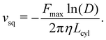 | (18) |
This result is independent of Lcap. The dependence on D is shown in Fig. 3. As expected, the swimming velocity goes to zero for D → 1 for a swimmer with a finite propulsion force. Also, the velocity diverges in the absence of confinement, which is an artifact of the theoretical model related to the fact that Fcyl vanishes as D → 0. This means that the model predicts zero fluid friction on a moving swimmer in the limit of D → 0, suggesting that the model should not be used for D ≪ 1. Furthermore, the ability of real swimmers is always limited by a finite value of the imposed surface velocity.
 |
| | Fig. 3 Velocity vsq of a freely moving cylindrical swimmer with a fixed propulsion force of Fmax = 0.14Fsph (Fsph = 6πηrcylucyl) as a function of confinement D for different swimmer lengths. The confinement D = rcyl/Rcap is varied by changing Rcap. | |
3.3 Squirmer motion in a closed capillary tube
Another situation is when the confinement geometry is closed, representing two dead ends. For instance, this is the case for swimmers in lipid vesicles located at the end of formed tethers.8,9 When the center of mass of the swimmer is tethered by a spring, mass conservation corresponds to zero fluid flux through the gap between the swimmer and the capillary tube, and reads  . In combination with the BCs u(Rcap) = 0 and u(rcyl) = ucyl, we can determine the parameters c1, c2, and Δp in eqn (10), leading to a solution for the flow profile in the gap and the resulting propulsion force
| |  | (19) |
The dependence of Fcyl on D is shown in Fig. 4(a) for different Lcyl. The propulsion force increases with increasing confinement, and diverges as rcyl/Rcap → 1. Similar to the case of the periodic tube, longer swimmers generate more thrust.
 |
| | Fig. 4 Approximate analytical model for a cylindrical swimmer in a capillary tube. (a) Propulsion force Fcyl of a spring-pinned swimmer in a closed tube as a function of confinement D for different swimmer lengths. The confinement D = rcyl/Rcap is varied by changing Rcap and the force is normalized by Fsph = 6πηrcylucyl. (b) Velocity vsq of a freely moving cylindrical swimmer in a closed tube far away from both tube ends and in an open tube with periodic BCs as a function of confinement D. | |
To determine the dependence of swimming velocity on D, the tethering spring is removed. For a freely-moving swimmer in a closed tube, the mass conservation reads  resulting in the swimming velocity
| |  | (20) |
Fig. 4(b) shows that the velocity decreases with increasing confinement and vanishes as
D → 1, despite an increasing propulsion force in
Fig. 4(a). Since we study a force-free swimmer, for which the propulsion force is equal to the drag force at a steady swimming velocity, the only possibility is that the drag force on the swimmer increases faster than its propulsion force as a function of
D. When we consider the case of
D = 1, the fluid exchange between the region anterior and posterior of the swimmer vanishes. For an incompressible fluid, the flow through the gap must also vanish due to volume conservation. This also explains the different behavior in comparison to the periodic tube, where the swimmer can “push” the fluid in front and hence can swim with a non-zero velocity. Note that the force and velocity of the swimmer in the closed tube are independent of the capillary length, since mass conservation is only affected by the flow in the gap between the swimmer and the capillary wall.
In order to compare the approximate analytical model for a closed tube with that of a periodic tube, Fig. 4(b) presents the velocity of a cylindrical swimmer as a function of confinement for the both models. In the limit of Lcap → ∞, the analytical model with periodic BCs along the capillary axis converges to that for a closed tube. As the capillary length increases, the overall resistance for fluid flow also increases, leading to a negligible volumetric flow rate within the tube for large capillary lengths.
A calculation based on a fixed propulsion force is similar to that for a capillary tube with periodic BCs in Section 3.2. Therefore, the predictions for Fcyl = Fmax in a closed capillary tube do not differ qualitatively from those in Fig. 3.
4 Simulations of spherical and spheroidal squirmer motion in cylindrical microchannels
In order to verify to which extent the approximate analytical model captures the behavior of squirmer in microchannels, we perform numerical simulations of a swimmer in a capillary tube for various conditions. In simulations, we use either spherical or spheroidal squirmer models, as described in Section 2.1. The results in Sections 4.1 and 4.2 are based on a neutral squirmer model (β = 0), while Section 4.3 analyses the effect of different swimming modes.
4.1 Simulation of a squirmer in a periodic capillary tube
A spring-fixed squirmer, whose center of mass is subject to a harmonic spring force F = −kz, starts swimming and comes to a halt when its propulsion force is equal to the spring force. This setup is used to measure the propulsion force of the squirmer. Fig. 5 compares the fluid velocity profile in the gap obtained from a simulation with the corresponding analytical prediction in eqn (11) for rcyl = rsq (rsq is the squirmer radius). The velocity is normalized by  which is the swimming velocity of a squirmer without confinement (or when rsq/Rcap → 0). The qualitative characteristics of ugap(r) are in a good agreement between the simulation and theory. Under the assumption that the cylinder length is equal to the squirmer diameter (i.e. Lcyl = 2rsq), flow velocity in the gap is slightly faster for the analytical model than in the simulation. When we do not fix Lcyl, but use it as a fitting parameter, the best fit between the theory and simulation is found for Lcyl = 1.41rsq. This value is somewhat smaller than the diameter of the squirmer, consistent with our expectations.
 |
| | Fig. 5 Flow velocity profile ugap(r) at the symmetry plane (z = 0) of a spherical swimmer. The confining capillary tube is periodic along its axis and the velocity is normalized by  which is the swimming velocity of a squirmer without confinement. Here, the confinement is D = rsq/Rcap = 0.56. The blue curve corresponds to averaged velocity profile from the simulation, while the red and orange lines represent velocity profiles from the analytical solution in eqn (11) for a cylinder with a radius rcyl = rsq, ucyl = −B1 and lengths Lcyl = 2rsq and Lcyl = 1.41rsq, respectively. which is the swimming velocity of a squirmer without confinement. Here, the confinement is D = rsq/Rcap = 0.56. The blue curve corresponds to averaged velocity profile from the simulation, while the red and orange lines represent velocity profiles from the analytical solution in eqn (11) for a cylinder with a radius rcyl = rsq, ucyl = −B1 and lengths Lcyl = 2rsq and Lcyl = 1.41rsq, respectively. | |
The extension of the spring by the spring-pinned squirmer allows the quantification of the propulsion force Fsq. Fig. 6(a) presents the dependence of Fsq on the confinement D. As expected from the approximate analytical model in eqn (15), Fsq increases with increasing D. Comparison of the simulation results with the analytical solution shows a good agreement for a fitted cylinder length of Lcyl = 1.22rsq, while the choice of Lcyl = 2rsq in eqn (15) results in the overprediction of the propulsion force measured in simulations. Fig. 6(b) shows an increase in the propulsion force of the squirmer as a function of the capillary length Lcap, which can be fitted well by the analytical model with Lcyl = 1.25rsq. The increase in Fsq with increasing Lcap is likely due to an increased friction for fluid flow in longer capillaries, which leads to slower flow velocities within the tube and more efficient swimmer propulsion. In the periodic capillary tube, the squirmer propulsion might be affected by its periodic images. For large capillary lengths, this effect is negligible, while it becomes increasingly relevant for Lcap ≲ 4rsq. Note that the effect of periodic images is not considered in the analytical model.
 |
| | Fig. 6 (a) and (b) Propulsion force Fsq of a spring-fixed spherical squirmer in comparison with the analytical prediction from eqn (15) for (a) different confinements D = rsq/Rcap with Lcap = 6rsq and (b) various capillary tube lengths Lcap with D = 0.56. The red and orange lines show propulsion forces from the analytical solution in eqn (15) for a cylindrical swimmer with radius rcyl = rsq, surface velocity ucyl = −B1 and two different lengths. The force is normalized by F0 = 6πηrsqv0 with  . (c) and (d) Swimming velocity vsq of the squirmer in comparison with the analytical prediction from eqn (16) for (c) different confinements D = rsq/Rcap with Lcap = 6rsq and (d) various capillary lengths Lcap with D = 0.56. The velocity is normalized by v0. The orange line corresponds to the analytical solution from eqn (16) for a cylinder with a radius rcyl = rsq, a surface velocity ucyl = −v0 and a cylinder length Lcyl = 2rsq. Fitting the cylinder length results in the same value. The green curve in (c) shows the swimming velocity at strong confinements from simulations with an increased fluid resolution (i.e. particle density n = 20/rc3). The confinement is varied by changing Rcap. The error bars represent standard deviation of simulation measurements. Periodic BCs in the z direction are assumed in all cases. . (c) and (d) Swimming velocity vsq of the squirmer in comparison with the analytical prediction from eqn (16) for (c) different confinements D = rsq/Rcap with Lcap = 6rsq and (d) various capillary lengths Lcap with D = 0.56. The velocity is normalized by v0. The orange line corresponds to the analytical solution from eqn (16) for a cylinder with a radius rcyl = rsq, a surface velocity ucyl = −v0 and a cylinder length Lcyl = 2rsq. Fitting the cylinder length results in the same value. The green curve in (c) shows the swimming velocity at strong confinements from simulations with an increased fluid resolution (i.e. particle density n = 20/rc3). The confinement is varied by changing Rcap. The error bars represent standard deviation of simulation measurements. Periodic BCs in the z direction are assumed in all cases. | |
Fig. 6(c) and (d) show the swimming velocity of a free squirmer as a function of D and Lcap. As expected, all simulated velocities of the squirmer are smaller than  for a squirmer in an unbounded fluid. The description of the simulation data by the analytical model from eqn (16) is less accurate here. We choose ucyl such that the swimming velocity of the theoretical model matches the bulk velocity of a squirmer for D → 0. At high confinement, there seems to be a qualitative disagreement between simulations and the analytical model [see Fig. 6(c)], which is due to an insufficient fluid resolution in simulations when the gap between the squirmer and the tube becomes very narrow. We have performed simulations with a four times larger fluid density (n = 20/rc3), which show that the nominal resolution with n = 5/rc3 is sufficient only up to confinements of D ≲ 0.75. Simulations with the finer resolution do reproduce an increase in vsq at large confinements, in qualitative agreement with the analytical model. Furthermore, our swimming velocity converges for increasing capillary length to that in ref. 26, where the swimming velocity of vsq = 0.8v0 was found for the confinement of D = 0.5.
We have also performed a few simulations using a spheroidal squirmer for intermediate confinements (see Fig. S1, ESI†). The qualitative trends of spheroidal squirmer motion as a function of confinement are the same as for the spherically-shaped squirmer, in agreement with the theoretical model. The optimal aspect ratio of the cylindrical swimmer from the analytical model to quantitatively capture the dependence of swimming velocity and propulsion force on the confinement D for the spheroidal swimmer with aspect ratio 2 increases roughly by the same factor compared to a spherical squirmer, as should be expected if the correspondence of the two models is not just fortuitous. Further simulations showed that the swimming velocity of the spheroidal squirmer is larger than for the spherical case, which is in agreement with theoretical predictions.34
4.2 Simulation of a squirmer in a closed capillary tube
Fig. 7(a) shows the propulsion force of a spherical spring-pinned squirmer in a closed tube as a function of confinement. The generated force increases with increasing rsq/Rcap and the correspondence between simulations and the analytical model in eqn (19) is good for Lcyl = 1.35rsq. Fig. 7(b) presents the swimming velocity of a neutral squirmer as a function of the distance between its center of mass and the wall at the positive end of the tube for different confinements. The swimming velocity becomes slower in more confined systems. Interestingly, the effect of the wall at the positive end of the tube on swimming velocity becomes relevant only for a distance d ≲ 1.5rsq, corresponding to a distance of half a radius between the wall and the squirmer surface. This indicates that the flow field generated by the squirmer is local and does not extend beyond the distance of 0.5rsq − 0.8rsq away from the squirmer surface. Note that d can be slightly lower than rsq, because the squirmer slightly deforms when it directly interacts with the wall. Nevertheless, away from the wall the squirmer shape remains spherical.
 |
| | Fig. 7 (a) Propulsion force Fsq of a spring-fixed spherical squirmer as a function of D = rsq/Rcap in a closed capillary tube. Simulation results (blue) are compared with the analytical solution (red and orange) from eqn (19) for two different cylinder lengths and a surface velocity ucyl = −B1. (b) and (c) Swimming velocity vsq of a free squirmer in a closed tube normalized by  . (b) vsq as a function of the distance d from the squirmer's center of mass to the closed end of the tube. Different colors represent different capillary radii, changing the confinement. The vertical red line indicates the distance at which the squirmer touches the wall. (c) Squirmer velocity away from the tube ends (averaged within the region 0.2rsq ≤ z ≤ rsq) in comparison with the analytical model from eqn (20) for ucyl = −v0. Simulation results are presented for different fluid resolutions with n = 5/rc3 (blue) and n = 20/rc3 (green). . (b) vsq as a function of the distance d from the squirmer's center of mass to the closed end of the tube. Different colors represent different capillary radii, changing the confinement. The vertical red line indicates the distance at which the squirmer touches the wall. (c) Squirmer velocity away from the tube ends (averaged within the region 0.2rsq ≤ z ≤ rsq) in comparison with the analytical model from eqn (20) for ucyl = −v0. Simulation results are presented for different fluid resolutions with n = 5/rc3 (blue) and n = 20/rc3 (green). | |
Fig. 7(c) compares the squirmer velocity for d > rsq with the results of the analytical model from eqn (20). The swimming velocity reduces with increasing confinement for both simulations and the analytical model, but simulations display overall larger velocities. Note that for confinements D > 0.75, we employ simulations with an increased fluid resolution (n = 20/rc3). A few simulations with a spheroidal squirmer shape show qualitatively similar behavior of the propulsion force and the swimming velocity as for the case of spherical squirmer. These results further support the validity of the proposed approximate analytical model of squirmer propulsion under confinement.
4.3 Effect of the swimming mode on squirmer behavior
All simulations described in Sections 4.1 and 4.2 are for a neutral squirmer with β = 0 (or B2 = 0), for which the slip velocity field is symmetric with respect to the squirmer's center of mass. Other swimming modes are obtained by varying the parameter β, which generates pusher (β < 0) and puller (β > 0) modes, where the thrust is generated predominantly in the front and in the back of the squirmer, respectively. Note that β ≠ 0 affects local flow field around the squirmer, but does not change its swimming velocity in an unbounded fluid. However, β strongly affects the interaction of the squirmer with walls and other swimmers.16,49,50 For example, a recent simulation study has shown that the swimmer navigation through a regular lattice of solid spheres depends on the swimming mode of microswimmers.51 It is important to note that the proposed analytical model does not include the effect of β ≠ 0.
In a capillary tube with periodic BCs, the propulsion force only weakly depends on the swimming mode with Fpuller/Fneutral = 1.02 and Fpusher/Fneutral = 0.99 for β = ±5 and Rcap = 2rsq. The ratios of swimming velocities are vpuller/vneutral = 0.98 and vpusher/vneutral = 1.08, so that pushers are slightly faster than pullers in a periodic capillary.
Further, we focus on the case of the closed capillary tube, and the propulsion of squirmers as they approach the closed ends. Fig. 8 shows flow fields around the squirmer spring-anchored at zanchor = rsq for different swimming modes. The flow fields are qualitatively different, and are significantly affected by confining walls. Fig. 9 presents propulsion forces of different squirmers anchored at various positions zanchor along the tube axis. When the squirmer is far enough (Lcap/2 − |zanchor| ≳ 1.5rsq) from the closed ends of the capillary, its propulsion force is independent of the anchoring position. The propulsion force of the neutral squirmer increases as the squirmer approaches the front end of the tube. The increase in Fsq for the neutral squirmer appears to be similar for the both tube ends, indicating that the squirmer interaction with the walls is independent of whether it swims away from or toward one of the closed ends. This is likely due to the symmetry of the local flow field around the neutral squirmer along its propulsion direction. When the squirmer is fixed at the center of the tube, Fsq is slightly larger (smaller) for the pusher (puller) in comparison to the neutral squirmer. The puller generates larger propulsion forces than the neutral squirmer when approaching the closed end in swimming direction. However, when the squirmer swims away from the capillary end, the puller is weaker than the neutral squirmer. Swimmer interaction with the closed ends is opposite for pushers in comparison with pullers. The pusher generates larger propulsion forces when it moves away from the tube end, and smaller forces when it moves toward the end in comparison to those of the neutral squirmer. This is not entirely surprising, because the asymmetry of the generated flow field is directed toward the front for pullers and toward the back for pushers. We have also verified that spheroidally-shaped squirmers exhibit qualitatively similar behavior in a closed capillary tube for different swimming modes.
 |
| | Fig. 8 Flow field around a spherical squirmer (grey) within a closed capillary tube with a length of Lcap = 6rsq and a radius of Rcap = 2rsq. The squirmer is tethered by a spring at the anchoring point with zanchor = rsq. The colors code the flow velocity in the z direction normalized by  . The red arrows represent flow lines within the y–z-plane. From the top to the bottom, the figures correspond to pusher (β = −5), neutral (β = 0), and puller (β = 5) squirmers. . The red arrows represent flow lines within the y–z-plane. From the top to the bottom, the figures correspond to pusher (β = −5), neutral (β = 0), and puller (β = 5) squirmers. | |
 |
| | Fig. 9 Propulsion force Fsq of a spherical spring-fixed squirmer as a function of its anchoring position zanchor for different swimming modes in a closed capillary tube with Lcap = 6rsq and Rcap = 2rsq. zanchor = 0 corresponds to the anchoring point in the middle of the tube length. The swimming orientation of the squirmer is always in the positive z direction, while the anchoring point also includes negative z values. The colors represent various swimming modes with different β values. | |
5 Discussion and conclusions
We have derived an approximate analytical solution for the propulsion of a cylindrical squirmer under confinement, and compared it to simulations of spherical and spheroidal squirmers moving inside a capillary tube. Both the analytical model and simulations show that the locomotion of squirmers is possible in cylindrical capillaries even under very strong confinement. For squirmers, the propulsion force increases with increasing confinement, and diverges as rcyl/Rcap → 1, according to predictions of the analytical model. This is in qualitative agreement with theoretical calculations for a swimmer near a wall.52 Despite the fact that the propulsion force may become very large under strong confinements, the swimming velocity can never exceed the velocity of a swimmer in an unbound fluid for rsq/Rcap → 0. This indicates that the fluid resistance generally grows faster than the propulsion force with increasing confinement, due to the assumption of a force-free swimmer.
The modeled swimmers generate their propulsion through the prescribed surface velocity, which results in large propulsion forces under strong confinements, independently of the magnitude of fluid resistance. In the theoretical model, these swimmers can generate an infinite power, which is clearly not the case for real biological or synthetic microswimmers, whose ability to generate propulsion has an upper limit. This indicates that real microswimmers would likely move slower under strong confinement in comparison to the predictions by the squirmer model, or may even stop moving for a fixed propulsion force when rsq/Rcap → 1.53 Note that the case where motion is implemented through the application of propulsion force of limited strength, instead of a prescribed surface slip velocity, has also been investigated.43–45 This corresponds to the analytical results for fixed propulsion described in Section 3.2. Furthermore, details of the local flow field generated by a microswimmer are important for its propulsion through confinements and crowded environments.54,55 Since biological swimmers generally propel due to the motion of attached appendages such as flagella and cilia, steric interactions between the appendages and surrounding walls can also affect the navigation of microswimmers through crowded environments.54 To accurately capture the complex interactions between microswimmers and their environment, more realistic models of biological swimmers with explicit appendages are required.
An important result of our investigation is that the generation of propulsion forces by squirmers under confinement is very localized, and can be thought of as ‘pushing forward’ using the walls, which occurs due to the interaction of local flow field generated by the swimmer with the walls. This is well supported by a short distance beyond which the generated flow field vanishes, see Fig. 8, and by the fact that the presence of closed tube ends is not important if the swimmer is more than its radius away from them. Therefore, microswimmers employ predominantly the closest confining walls around them to propel forward. Also, this means that specific geometric details of a confining environment are increasingly important close to the swimmer, and become irrelevant further away from it. Furthermore, the locality of force generation is relevant for the understanding of tether pulling from fluid membrane vesicles by enclosed microswimmers.8,9,29 For instance, we conclude that a squirmer-like swimmer cannot pull long tethers, because when the squirmer becomes fully and closely surrounded by the membrane after tether initiation, the generated force cannot propagate anymore toward the vesicle through the tether in order to further extend it. Furthermore, the force on the tether end is compensated by an opposing force on the tether walls. In a recent experiment of Bacillus subtilis bacteria in fluid vesicles, relatively short tethers filled by a train-like arrangement of 2–3 bacteria are formed.8 It is likely due to sequential entering of bacteria, such that the first initiates a tether of approximately its own length, then a second bacterium extends it by another bacterium length, etc. In another experiment,29E. coli bacteria were able to pull relatively long tethers due to another mechanism, where E. coli helical flagella form a single bundle, which is tightly wrapped by the membrane after tether formation, so that the membrane-wrapped bundle serves as a propeller to move forward and extend the tether.
Our simulations show that strong confinements may require a fine resolution to accurately capture fluid flow between the swimmer and the wall, which is associated with large computational costs. Furthermore, fluid compressibility may play an important role for systems with strong confinements, as large pressure gradients develop. The DPD method has a limited control over the fluid compressibility, which can be improved by using the smoothed dissipative particle dynamics method,56,57 where the equation of state can be prescribed explicitly.
Author contributions
G. G. and D. A. F. conceived the research project. F. A. O. and D. A. F. developed the analytical model. F. A. O. performed the simulations and analysed the obtained data. All authors participated in the discussions and writing of the manuscript.
Conflicts of interest
There are no conflicts to declare.
Appendices
Appendix A: Spheroidal squirmer model
For the derivation of analytical expressions, it is convenient to work in modified prolate spheroidal coordinates58ζ ∈ [1, −1], τ ∈ [1, ∞], and ϕ ∈ [0, 2π], whose relation to the Cartesian coordinates is given by| |  | (21) |
where 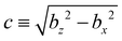 is the geometric constant which controls spheroid eccentricity e = c/bz. Normal (n = eτ) and tangential (t = −eζ) vectors at the spheroid surface are given by
| |  | (22) |
The surface velocity of a spheroidal squirmer is then34| | | usurf = −B1(1 + βζ)(t·ez)t, | (23) |
where β = B2/B1 and ez = (0,0,1)T.
Appendix B: Expressions for the parameters of the approximate analytical model for cylindrical microswimmers
Parameters for the case of a spring-fixed swimmer in a periodic capillary tube are given by| |  | (24) |
For a free cylindrical swimmer in a periodic capillary tube, the parameters are
| |  | (25) |
Parameters for the case of a spring-pinned swimmer in a closed capillary tube are given by
| |  | (26) |
For a free cylindrical swimmer in a closed capillary tube, the parameters are
| |  | (27) |
Acknowledgements
Support by the Deutsche Forschungsgemeinschaft (DFG) within the Priority Programme “Physics of Parasitism” (SPP 2332) is gratefully acknowledged. The authors gratefully appreciate computing time on the supercomputer JURECA59 at Forschungszentrum Jülich under grant no. actsys.
Notes and references
- J. Elgeti, R. G. Winkler and G. Gompper, Rep. Prog. Phys., 2015, 78, 056601 CrossRef CAS PubMed.
- C. Bechinger, R. Di Leonardo, H. Löwen, C. Reichhardt, G. Volpe and G. Volpe, Rev. Mod. Phys., 2016, 88, 045006 CrossRef.
- G. E. Kaiser and R. N. Doetsch, Nature, 1975, 255, 656–657 CrossRef CAS PubMed.
- A. Nsamela, P. Sharan, A. Garcia-Zintzun, S. Heckel, P. Chattopadhyay, L. Wang, M. Wittmann, T. Gemming, J. Saenz and J. Simmchen, ChemNanoMat, 2021, 7, 1042–1050 CrossRef CAS.
- C.-K. Tung, C. Lin, B. Harvey, A. G. Fiore, F. Ardon, M. Wu and S. S. Suarez, Sci. Rep., 2017, 7, 3152 CrossRef PubMed.
- T. Krüger, S. Schuster and M. Engstler, Trends Parasitol., 2018, 34, 1056–1067 CrossRef PubMed.
- T. Bhattacharjee and S. S. Datta, Nat. Commun., 2019, 10, 2075 CrossRef PubMed.
- S. C. Takatori and A. Sahu, Phys. Rev. Lett., 2020, 124, 158102 CrossRef CAS PubMed.
- H. R. Vutukuri, M. Hoore, C. Abaurrea-Velasco, L. van Buren, A. Dutto, T. Auth, D. A. Fedosov, G. Gompper and J. Vermant, Nature, 2020, 586, 52–56 CrossRef CAS PubMed.
- J. Elgeti and G. Gompper, Eur. Phys. J. Special Topics, 2016, 225, 2333–2352 CrossRef.
- S. Jana, S. H. Um and S. Jung, Phys. Fluids, 2012, 24, 041901 CrossRef.
- S. Palagi and P. Fischer, Nat. Rev. Mater., 2018, 3, 113–124 CrossRef CAS.
- M. Medina-Sánchez, V. Magdanz, M. Guix, V. M. Fomin and O. G. Schmidt, Adv. Funct. Mater., 2018, 28, 1707228 CrossRef.
- J. Elgeti and G. Gompper, Proc. Natl. Acad. Sci. U. S. A., 2013, 110, 4470–4475 CrossRef CAS PubMed.
- H. H. Wensink and H. Löwen, Phys. Rev. E: Stat., Nonlinear, Soft Matter Phys., 2008, 78, 031409 CrossRef CAS PubMed.
- A. P. Berke, L. Turner, H. C. Berg and E. Lauga, Phys. Rev. Lett., 2008, 101, 038102 CrossRef PubMed.
- J. Elgeti and G. Gompper, Europhys. Lett., 2013, 101, 48003 CrossRef CAS.
- Y. Fily, A. Baskaran and M. F. Hagan, Soft Matter, 2014, 10, 5609–5617 RSC.
- Y. Fily, A. Baskaran and M. F. Hagan, Phys. Rev. E: Stat., Nonlinear, Soft Matter Phys., 2015, 91, 012125 CrossRef PubMed.
- P. Iyer, R. G. Winkler, D. A. Fedosov and G. Gompper, Phys. Rev. Res., 2023, 5, 033054 CrossRef CAS.
- I. D. Vladescu, E. J. Marsden, J. Schwarz-Linek, V. A. Martinez, J. Arlt, A. N. Morozov, D. Marenduzzo, M. E. Cates and W. C. K. Poon, Phys. Rev. Lett., 2014, 113, 268101 CrossRef CAS PubMed.
- S. Rode, J. Elgeti and G. Gompper, New J. Phys., 2019, 21, 013016 CrossRef.
- L. Turner, W. S. Ryu and H. C. Berg, J. Bacteriol., 2000, 182, 2793–2801 CrossRef CAS PubMed.
- J. L. Bargul, J. Jung, F. A. McOdimba, C. O. Omogo, V. O. Adung'a, T. Krüger, D. K. Masiga and M. Engstler, PLoS Pathog., 2016, 12, e1005448 CrossRef PubMed.
- N. Heddergott, T. Krüger, S. B. Babu, A. Wei, E. Stellamanns, S. Uppaluri, T. Pfohl, H. Stark and M. Engstler, PLoS Pathog., 2012, 8, e1003023 CrossRef CAS PubMed.
- L. Zhu, E. Lauga and L. Brandt, J. Fluid Mech., 2013, 726, 285–311 CrossRef.
- B. Liu, K. S. Breuer and T. R. Powers, Phys. Fluids, 2014, 26, 011701 CrossRef.
- A. Creppy, E. Clément, C. Douarche, M. V. D'Angelo and H. Auradou, Phys. Rev. Fluids, 2019, 4, 013102 CrossRef.
- L. Le Nagard, A. T. Brown, A. Dawson, V. A. Martinez, W. C. K. Poon and M. Staykova, Proc. Natl. Acad. Sci. U. S. A., 2022, 119, e2206096119 CrossRef CAS PubMed.
- P. Iyer, G. Gompper and D. A. Fedosov, Soft Matter, 2022, 18, 6868–6881 RSC.
- M. J. Lighthill, Commun. Pure Appl. Math., 1952, 5, 109–118 CrossRef.
- J. R. Blake, J. Fluid Mech., 1971, 46, 199–208 CrossRef.
- F. Alarcón, C. Valeriani and I. Pagonabarraga, Soft Matter, 2017, 13, 814–826 RSC.
- M. Theers, E. Westphal, G. Gompper and R. G. Winkler, Soft Matter, 2016, 12, 7372–7385 RSC.
- P. J. Hoogerbrugge and J. M. V. A. Koelman, Europhys. Lett., 1992, 19, 155–160 CrossRef.
- P. Español and P. Warren, Europhys. Lett., 1995, 30, 191–196 CrossRef.
- P. Español and P. B. Warren, J. Chem. Phys., 2017, 146, 150901 CrossRef PubMed.
- D. A. Fedosov, B. Caswell and G. E. Karniadakis, Biophys. J., 2010, 98, 2215–2225 CrossRef CAS PubMed.
- D. A. Fedosov, H. Noguchi and G. Gompper, Biomech. Model. Mechanobiol., 2014, 13, 239–258 CrossRef PubMed.
- W. Helfrich, Z. Naturforsch., 1973, 28, 693–703 CrossRef CAS PubMed.
-
G. Gompper and D. M. Kroll, Statistical mechanics of membranes and surfaces, World Scientific, Singapore, 2nd edn, 2004, pp. 359–426 Search PubMed.
- M. Revenga, I. Zúñiga, P. Español and I. Pagonabarraga, Int. J. Mod. Phys. C, 1998, 9, 1319–1328 CrossRef.
- S. Xiao, H.-Y. Chen, Y.-J. Sheng and H.-K. Tsao, Soft Matter, 2015, 11, 2416–2422 RSC.
- C. M. Barriuso Gutiérrez, J. Martn-Roca, V. Bianco, I. Pagonabarraga and C. Valeriani, Front. Phys., 2022, 10, 926609 CrossRef.
- M. R. Bailey, C. M. Barriuso Gutiérrez, J. Martn-Roca, V. Niggel, V. Carrasco-Fadanelli, I. Buttinoni, I. Pagonabarraga, L. Isa and C. Valeriani, Nanoscale, 2024, 16, 2444–2451 RSC.
- J. A. Backer, C. P. Lowe, H. C. J. Hoefsloot and P. D. Iedema, J. Chem. Phys., 2005, 122, 154503 CrossRef CAS PubMed.
- D. A. Fedosov, G. E. Karniadakis and B. Caswell, J. Chem. Phys., 2010, 132, 144103 CrossRef PubMed.
- H. A. Stone and A. D. T. Samuel, Phys. Rev. Lett., 1996, 77, 4102–4104 CrossRef CAS PubMed.
- I. O. Götze and G. Gompper, Phys. Rev. E: Stat., Nonlinear, Soft Matter Phys., 2010, 82, 041921 CrossRef PubMed.
- A. Zöttl and H. Stark, Phys. Rev. Lett., 2012, 108, 218104 CrossRef PubMed.
- A. Chamolly, T. Ishikawa and E. Lauga, New J. Phys., 2017, 19, 115001 CrossRef.
- T. Ishikawa, J. Appl. Phys., 2019, 125, 200901 CrossRef.
- A. Gürbüz, A. Lemus, E. Demir, O. S. Pak and A. Daddi-Moussa-Ider, Phys. Fluids, 2023, 35, 081907 CrossRef.
- A. Acemoglu and S. Yesilyurt, Biophys. J., 2014, 106, 1537–1547 CrossRef CAS PubMed.
- B. U. Felderhof, Phys. Fluids, 2010, 22, 113604 CrossRef.
- P. Español and M. Revenga, Phys. Rev. E: Stat., Nonlinear, Soft Matter Phys., 2003, 67, 026705 CrossRef PubMed.
- K. Müller, D. A. Fedosov and G. Gompper, J. Comput. Phys., 2015, 281, 301–315 CrossRef.
- R. Pöhnl, M. N. Popescu and W. E. Uspal, J. Phys.: Condens. Matter, 2020, 32, 164001 CrossRef PubMed.
- Jülich Supercomputing Centre, J. Large-Scale Res. Facil., 2021, 7, A182 CrossRef.
Footnote |
| † Electronic supplementary information (ESI) available: A supplementary figure showing propulsion forces for a spheroidal squirmer in an open capillary tube. See DOI: https://doi.org/10.1039/d3sm01480k |
|
| This journal is © The Royal Society of Chemistry 2024 |
Click here to see how this site uses Cookies. View our privacy policy here. 
 Open Access Article
 This Open Access Article is licensed under a
  *,
Gerhard
Gompper
*,
Gerhard
Gompper
 . We use the ratio β = B2/B1 to capture the modality. For β > 0 the squirmer is called a puller, for β = 0 it is neutral and for β < 0 it is a pusher.
 for a spherical squirmer to v0 = B1 as a function of increasing aspect ratio of the spheroidal shape.34
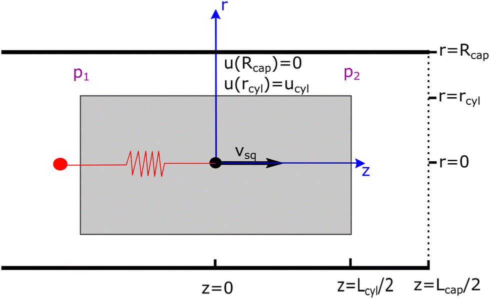


 where γ and σ are the force strength coefficients, vij = vi − vj, ξij = ξji is a Gaussian random variable with zero mean and unit variance, and Δt is the time step. The fluctuation–dissipation theorem relates these weight functions and the force coefficients as36

 is the discretized mean curvature at vertex i, ni is the unit normal at the membrane vertex i,
  is the area corresponding to vertex i (the area of the dual cell), j(i) corresponds to all vertices linked to vertex i, and σij = rij(cot


 s = 1 for ωC and s = 0.1 for ωD and ωR, where m = 1 is the particle mass and kBT = 1 is the unit of energy. This results in a fluid dynamic viscosity of
  which is computed in a separate simulation using the reverse Poiseuille flow approach.46,47 Coupling between the spherical squirmer and fluid particles assumes asf = 0 and
  with rsfc = 0.8rc. The value of γsf is computed such that the imposed slip BCs at the squirmer surface are obtained.38 For the spheroidal swimmer,
  because the surface density of squirmer particles is different from that for the spherical swimmer. For simulations with a finer fluid resolution, the density is set to n = 20/rc3, while the cutoff radius is
  to reduce the overall computational cost. In this case, the dynamic viscosity becomes
  which is close to that in simulations with n = 5/rc3. The time step is
  and the center of mass of the squirmer is sampled every 100 time steps. The velocity is computed using the distance that the swimmer covers within 800 time steps. Error bars represent the standard deviation of these samples.


 with ϕ denoting the polar angle. This allows us to compute Δp and fully determine the flow profiles above.
 with surface normal n. In cylindrical coordinates with the assumption that ur = uϕ = 0, the stress tensor becomes


 at the cylinder jacket vanishes as Rcap → ∞ (or D → 0), so that the shear stress on the cylinder also disappears.
 . As a result, we obtain the swimming velocity


 . In combination with the BCs u(Rcap) = 0 and u(rcyl) = ucyl, we can determine the parameters c1, c2, and Δp in eqn (10), leading to a solution for the flow profile in the gap and the resulting propulsion force
 resulting in the swimming velocity
 which is the swimming velocity of a squirmer without confinement (or when rsq/Rcap → 0). The qualitative characteristics of ugap(r) are in a good agreement between the simulation and theory. Under the assumption that the cylinder length is equal to the squirmer diameter (i.e. Lcyl = 2rsq), flow velocity in the gap is slightly faster for the analytical model than in the simulation. When we do not fix Lcyl, but use it as a fitting parameter, the best fit between the theory and simulation is found for Lcyl = 1.41rsq. This value is somewhat smaller than the diameter of the squirmer, consistent with our expectations.

 which is the swimming velocity of a squirmer without confinement. Here, the confinement is D = rsq/Rcap = 0.56. The blue curve corresponds to averaged velocity profile from the simulation, while the red and orange lines represent velocity profiles from the analytical solution in eqn (11) for a cylinder with a radius rcyl = rsq, ucyl = −B1 and lengths Lcyl = 2rsq and Lcyl = 1.41rsq, respectively.
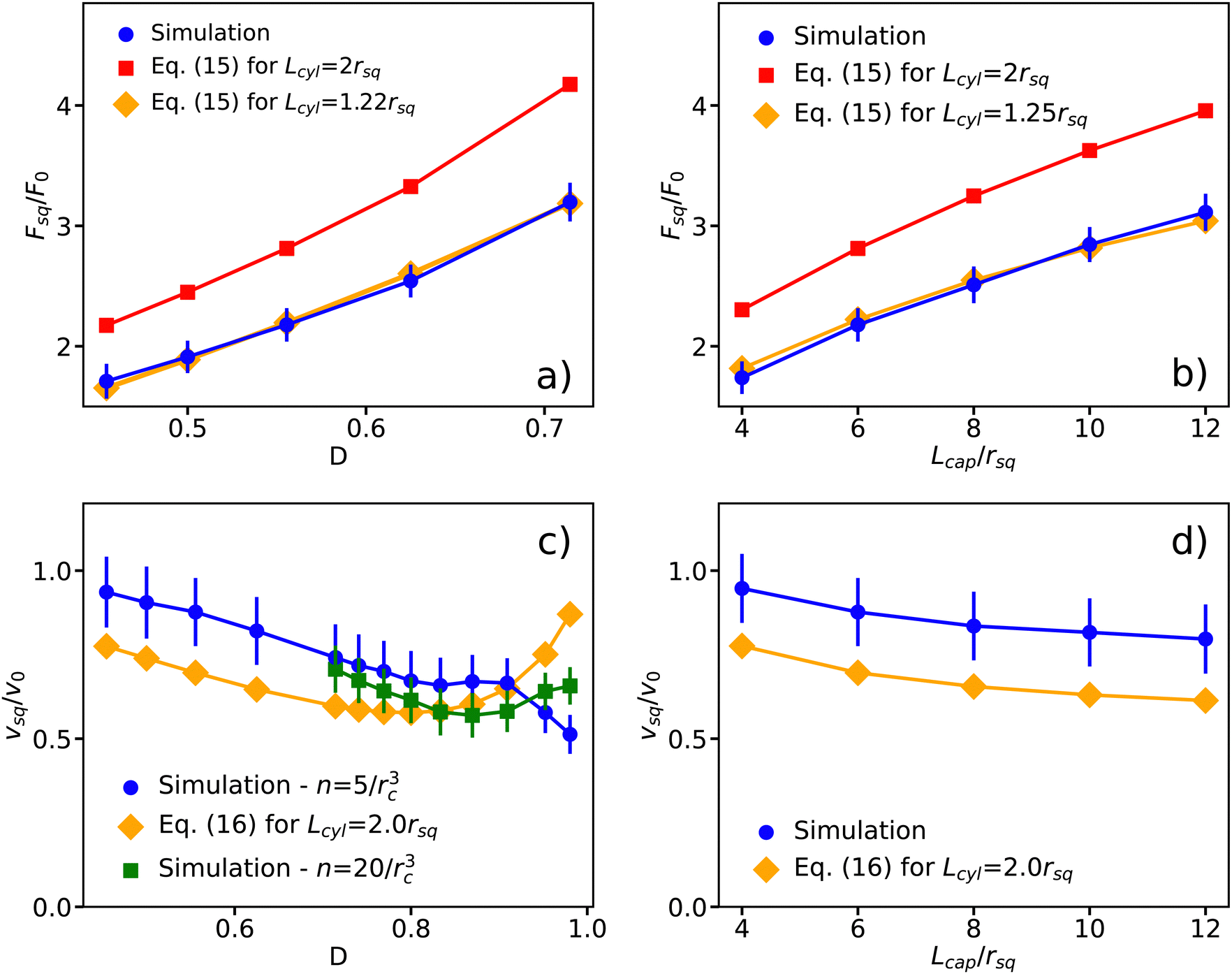
 . (c) and (d) Swimming velocity vsq of the squirmer in comparison with the analytical prediction from eqn (16) for (c) different confinements D = rsq/Rcap with Lcap = 6rsq and (d) various capillary lengths Lcap with D = 0.56. The velocity is normalized by v0. The orange line corresponds to the analytical solution from eqn (16) for a cylinder with a radius rcyl = rsq, a surface velocity ucyl = −v0 and a cylinder length Lcyl = 2rsq. Fitting the cylinder length results in the same value. The green curve in (c) shows the swimming velocity at strong confinements from simulations with an increased fluid resolution (i.e. particle density n = 20/rc3). The confinement is varied by changing Rcap. The error bars represent standard deviation of simulation measurements. Periodic BCs in the z direction are assumed in all cases.
 for a squirmer in an unbounded fluid. The description of the simulation data by the analytical model from eqn (16) is less accurate here. We choose ucyl such that the swimming velocity of the theoretical model matches the bulk velocity of a squirmer for D → 0. At high confinement, there seems to be a qualitative disagreement between simulations and the analytical model [see Fig. 6(c)], which is due to an insufficient fluid resolution in simulations when the gap between the squirmer and the tube becomes very narrow. We have performed simulations with a four times larger fluid density (n = 20/rc3), which show that the nominal resolution with n = 5/rc3 is sufficient only up to confinements of D ≲ 0.75. Simulations with the finer resolution do reproduce an increase in vsq at large confinements, in qualitative agreement with the analytical model. Furthermore, our swimming velocity converges for increasing capillary length to that in ref. 26, where the swimming velocity of vsq = 0.8v0 was found for the confinement of D = 0.5.
 . (b) vsq as a function of the distance d from the squirmer's center of mass to the closed end of the tube. Different colors represent different capillary radii, changing the confinement. The vertical red line indicates the distance at which the squirmer touches the wall. (c) Squirmer velocity away from the tube ends (averaged within the region 0.2rsq ≤ z ≤ rsq) in comparison with the analytical model from eqn (20) for ucyl = −v0. Simulation results are presented for different fluid resolutions with n = 5/rc3 (blue) and n = 20/rc3 (green).
 . The red arrows represent flow lines within the y–z-plane. From the top to the bottom, the figures correspond to pusher (β = −5), neutral (β = 0), and puller (β = 5) squirmers.

 is the geometric constant which controls spheroid eccentricity e = c/bz. Normal (n = eτ) and tangential (t = −eζ) vectors at the spheroid surface are given by


