
 Open Access Article
 This Open Access Article is licensed under a Creative Commons Attribution-Non Commercial 3.0 Unported Licence
Periodic table screening for enhanced positive contrast in MRI and in vivo uptake in glioblastoma†
Aitor
Herraiz
a,
M. Puerto
Morales
 b,
Lydia
Martínez-Parra
cde,
Nuria
Arias-Ramos
f,
Pilar
López-Larrubia
f,
Lucía
Gutiérrez
g,
Jesús
Mejías
a,
Carlos
Díaz-Ufano
b,
Jesús
Ruiz-Cabello
cdhi and
Fernando
Herranz
*ah
b,
Lydia
Martínez-Parra
cde,
Nuria
Arias-Ramos
f,
Pilar
López-Larrubia
f,
Lucía
Gutiérrez
g,
Jesús
Mejías
a,
Carlos
Díaz-Ufano
b,
Jesús
Ruiz-Cabello
cdhi and
Fernando
Herranz
*ah
aGrupo de Nanomedicina e Imagen Molecular, Instituto de Química Médica (IQM/CSIC), Juan de la Cierva 3, 28006 Madrid, Spain. E-mail: fherranz@iqm.csic.es
bDepartamento de Nanociencia y Nanotecnología, Instituto de Ciencia de Materiales de Madrid, CSIC, Sor Juana Inés de la Cruz 3. Cantoblanco, 28049 Madrid, Spain
cCIC biomaGUNE, Basque Research and Technology Alliance (BRTA, ), Paseo de Miramon 182, 20014, Donostia San Sebastián, Spain
dIkerbasque, Basque Foundation for Science, Plaza Euskadi 5, 4800 Bilbao, Spain
eMolecular Biology and Biochemistry Department, Universidad del País Vasco (UPV/EHU), Barrio Sarriena s/n, 48940 Leioa, Spain
fInstituto de Investigaciones Biomédicas Sols-Morreale (IIBM), CSIC-UAM, Madrid, Spain
gDepartamento de Química Analítica, Instituto de Nanociencia y Materiales de Aragón. Universidad de Zaragoza y CIBERBBN, Mariano Esquillor s/n, 50018, Zaragoza, Spain
hCIBER Enfermedades Respiratorias (CIBERES), Melchor Fernández-Almagro 3, 28029 Madrid, Spain
iNMR and Imaging in Biomedicine Group, Department of Chemistry in Pharmaceutical Sciences, Pharmacy School, University Complutense Madrid, 28040, Madrid, Spain
First published on 8th May 2024
Abstract
The quest for nanomaterial-based imaging probes that can provide positive contrast in MRI is fueled by the necessity of developing novel diagnostic applications with potential for clinical translation that current gold standard probes cannot provide. Although interest in nanomaterials for positive contrast has increased in recent years, their study is less developed than that of traditional negative contrast probes in MRI. In our search for new magnetic materials with enhanced features as positive contrast probes for MRI, we decided to explore the chemical space to comprehensively analyze the effects of different metals on the performance of iron oxide nanomaterials already able to provide positive contrast in MRI. To this end, we synthesized 30 different iron oxide-based nanomaterials. Thorough characterization was performed, including multivariate analysis, to study the effect of different variables on their relaxometric properties. Based on these results, we identified the best combination of metals for in vivo imaging and tested them in different experiments. First, we tested its performance on magnetic resonance angiography using a concentration ten times lower than that clinically approved for Gd. Finally, we studied the capability of these nanomaterials to cross the affected blood–brain barrier in a glioblastoma model. The results showed that the selected nanomaterials provided excellent positive contrast at large magnetic field and were able to accumulate at the tumor site, highlighting the affected tissue.
Introduction
In recent years, there has been considerable interest in employing iron oxide nanoparticles (IONP) as positive contrast agents in magnetic resonance imaging (MRI). This approach has gained attention because of its distinct benefits compared with the traditional T2-weighted dark contrast.1,2 For this reason, the modification of different physicochemical features of such particles has been tested, like fine tuning of the nanoparticle shape, composition, and coating. These are key factors in modulating the relaxometric values (r1 and r2/r1) that determine whether the probe is optimal for positive-contrast MRI. The exploration of core-doped IONP with different metals has primarily focused on enhancing their T2 capabilities, with less attention given to enhancing the T1 signal.3–6 The number of iron oxide nanoparticle-based T1 agents has been growing progressively over the past few years. Nevertheless, it is still relatively rare to find nanoparticles that exhibit substantial r1 values (at the standard 1 T magnetic fields) while also demonstrating optimal properties for in vivo experiments. To develop a useful IONP for T1-MR imaging, not only is a large r1 value at 1 T needed, but one must also demonstrate how the imaging is generated in vivo at a large, pre-clinical, field strength (7 T and higher).In the last few years we developed a new type of iron oxide nanomaterial showing excellent in vivo properties and large r1 values.7,8 However, the r1 value of these nanoparticles, which was 11.9 mM−1 s−1 (mM of Fe + Cu) at 1.5 T, has room for improvement. For example, introducing Cu2+ as the core dopant in this material led to an increase in the r1 value to 15.7 mM−1 s−1 at 1.5 T. Based on these results, we wanted to examine how the controlled addition of various metals could further extend the r1 limits. To achieve this goal, the first question was which metals were used in this study. Because exploring the effect of core doping in IONP and their relationship with r1 values is a scarcely studied field, we attempted to use as many metals as possible. Therefore, we used most of the metals in the periodic table, those that could be employed in our synthetic protocol, with 30 different nanomaterials tested as T1-MRI contrast agents. After analyzing their physicochemical properties, we opted to select those that offered diverse r1 values, spanning a broad range of outcomes, for further characterization. We synthesized all the nanoparticles using the same synthetic protocol and tested them in vivo. First, the selected nanomaterial was used in magnetic resonance angiography of healthy mice at a concentration ten times lower than that of clinically approved Gd compounds. Finally, this nanomaterial was used for in vivo uptake in glioblastoma in a mouse model, demonstrating its capacity to cross the affected blood–brain barrier.
Results and discussion
We studied the incorporation of 30 distinct metals into the core of extremely small iron oxide nanoparticles and examined their influence on their T1 capabilities.Several concentrations of each metal were tested, yielding 59 nanoparticles studied. The synthetic methodology was adapted from previous studies, replacing the use of microwaves with traditional plate heating at 120 °C and extending the reaction time until 45 min,7,8 together with hydrazine hydrate and, as coating molecule, sodium citrate. Once synthesized, we studied the hydrodynamic size, Z potential (ZPOT), magnetization saturation (MSAT), thermogravimetry, and relaxometry values of the successfully prepared nanoparticles. The generated data are presented in Table 1. This table shows the data for the IONP successfully prepared and only for the concentration showing the best value for r1, our final goal, a total of 30 nanoparticles. For clarity, the data obtained for the remaining 29 nanoparticles are not shown (see supp. info for more data).
| Metal | Added conc. (mM) | Incorporation (%) | Ratio[mM] [M]/[Fe] | Crystal size (Å) | Hydrodynamic size (nm) | Z pot. (mV) | % Coating | M SAT (A m2 kg−1) | r 1 (mM−1 s−1) | r 2 (mM−1 s−1) | r 2/r1 |
|---|---|---|---|---|---|---|---|---|---|---|---|
| IONP | — | — | — | 50.4 | 7.6 | −27.4 | 26.5 | 92.7 | 12.8 | 27.3 | 2.1 |
| Be2+ | 4.5 | 21.1 | 0.042 | 33.4 | 7.1 | −33.7 | 28.3 | 73.2 | 7.6 | 14.3 | 1.9 |
| Mg2+ | 1.5 | 10.3 | 0.006 | 35.5 | 10.9 | −27.5 | 25.1 | 87.9 | 13.6 | 26.8 | 2.0 |
| Al3+ | 4.5 | 53.8 | 0.117 | 35.4 | 6.6 | −32.2 | 32.0 | 66.2 | 6.5 | 13.4 | 2.0 |
| Ca2+ | 4.5 | 42.9 | 0.070 | 34.3 | 6.4 | −27.8 | 23.1 | 84.2 | 12.4 | 23.9 | 1.9 |
| Sc3+ | 4.5 | 20.8 | 0.033 | 40.1 | 8.3 | −22.1 | 28.6 | 81.0 | 12.1 | 25.7 | 2.1 |
| Cr3+ | 4.5 | 31.5 | 0.067 | 49.3 | 6.8 | −39.2 | 31.0 | 46.8 | 4.7 | 10.0 | 2.1 |
| Mn2+ | 4.5 | 44.0 | 0.085 | 38.9 | 7.4 | −24.6 | 33.2 | 82.1 | 11.2 | 25.4 | 2.3 |
| Ni2+ | 4.5 | 13.4 | 0.025 | 45.5 | 6.1 | −22.7 | 23.0 | 75.5 | 11.2 | 22.1 | 2.0 |
| Co2+ | 4.5 | 22.4 | 0.052 | 36.8 | 8.1 | −33.1 | 27.1 | 85.2 | 11.9 | 25.0 | 2.1 |
| Zn2+ | 1.5 | 97.1 | 0.058 | 37.0 | 6.6 | −33.4 | 25.2 | 98.5 | 17.4 | 33.8 | 1.8 |
| Ga3+ | 1.5 | 49.7 | 0.035 | 50.2 | 8.5 | −31.1 | 24.5 | 85.7 | 17.4 | 38.6 | 2.3 |
| Sr2+ | 1.5 | 34.8 | 0.025 | 38.0 | 8.7 | −38.7 | 26.6 | 80.6 | 15.3 | 30.1 | 2.0 |
| Y3+ | 4.5 | 26.5 | 0.069 | 37.2 | 6.1 | −28.0 | 44.4 | 52.5 | 4.8 | 10.1 | 2.1 |
| Zr4+ | 4.5 | 76.4 | 0.131 | 36.2 | 8.6 | −44.3 | 28.5 | 62.7 | 8.0 | 19.3 | 2.4 |
| Mo3+ | 4.5 | 3.5 | 0.007 | 39.5 | 7.0 | −29.3 | 31.9 | 78.4 | 9.9 | 19.6 | 2.0 |
| Cd2+ | 4.5 | 14.3 | 0.026 | 49.2 | 7.3 | −34.7 | 25.7 | 80.0 | 12.0 | 22.7 | 1.9 |
| Ba2+ | 4.5 | 22.8 | 0.051 | 44.3 | 7.7 | −28.0 | 23.3 | 63.3 | 10.9 | 22.5 | 2.1 |
| La3+ | 1.5 | 41.2 | 0.037 | 49.6 | 5.6 | −39.1 | 38.6 | 36.2 | 2.1 | 4.6 | 2.2 |
| Ce3+ | 1.5 | 66.7 | 0.068 | 53.2 | 4.0 | −32.0 | 47.3 | 16.2 | 0.4 | 0.8 | 1.9 |
| Sm3+ | 1.5 | 79.9 | 0.073 | 32.9 | 5.0 | −37.5 | 32.5 | 22.5 | 1.4 | 2.7 | 2.0 |
| Eu3+ | 1.5 | 51.2 | 0.040 | 32.8 | 6.6 | −35.3 | 27.7 | 72.6 | 3.4 | 7.9 | 2.3 |
| Gd3+ | 1.5 | 59.3 | 0.051 | 32.5 | 4.9 | −41.5 | 30.7 | 32.5 | 2.5 | 4.7 | 1.9 |
| Tb3+ | 4.5 | 40.8 | 0.098 | 38.9 | 6.1 | −39.1 | 42.6 | 39.1 | 1.8 | 3.7 | 2.1 |
| Dy3+ | 4.5 | 40.6 | 0.094 | 43.2 | 5.4 | −37.0 | 38.4 | 39.8 | 2.1 | 4.2 | 2.0 |
| Ho3+ | 4.5 | 30.7 | 0.071 | 33.8 | 6.6 | −38.3 | 32.2 | 38.1 | 4.1 | 8.3 | 2.0 |
| Er3+ | 4.5 | 31.2 | 0.071 | 33.7 | 6.3 | −37.5 | 27.4 | 39.3 | 4.0 | 8.0 | 2.0 |
| Tm3+ | 4.5 | 30.5 | 0.066 | 34.6 | 6.9 | −25.9 | 35.2 | 53.8 | 6.2 | 12.6 | 2.0 |
| Yb3+ | 4.5 | 40.8 | 0.077 | 38.2 | 6.2 | −36.7 | 28.0 | 52.1 | 5.7 | 11.4 | 2.0 |
| Lu3+ | 4.5 | 32.7 | 0.078 | 36.0 | 8.5 | −33.8 | 33.7 | 56.8 | 8.2 | 16.8 | 2.0 |
| Hf4+ | 4.5 | 46.4 | 0.088 | 38.4 | 10.3 | −36.5 | 27.4 | 68.4 | 12.9 | 30.1 | 2.3 |
Initial screening
Table 1 displays the concentration of each metal used in the reaction, percentage of incorporation, and final molar ratio of each metal to Fe. The concentrations tested were 1.5, 4.5, 7.0 and 10.0 mM. The initial value of 4.5 mM was selected based on previous results in the group using Cu2+ as the doping metal,9 and several higher and lower concentrations were added to explore the r1 values. However, we did not include larger concentrations of each metal because our goal was to finely tune the relaxometric properties of the nanoparticles without completely changing the original material. As shown in Table 1, only the concentration that provided the best r1 value is included for each metal.In general, the lower concentrations (1.5 mM and 4.5 mM) provided the best r1 values for each metal. The metal incorporation ranged from 3.4% using Mo3+ to 97.2% using Zn2+, with most metals showing incorporation levels in the 20–50% range. These results confirm the desired low metal-to-iron ratios for all the metals in the different samples. The next parameters assessed in this initial screening were crystal size, hydrodynamic size, zeta potential, and percentage of organic coating on the surface. To determine how doping with metal cations alters the crystal structure of the core, XRD characterization of all the samples was performed. All the samples showed a cubic inverse spinel-like structure corresponding to maghemite (γ – Fe2O3). However, XRD alone is not sufficient to discern maghemite/magnetite because of the similarity of both spectra; further characterization of the functional groups is necessary to demonstrate the obtained structure.10,11 Due to the special size of nanoparticles, on the order of a few nanometers, an approximate estimation of the crystal size (τ) was made using the Paul Scherrer equation.12 Further analysis of the functional groups of M-IONP was carried out using infrared spectroscopy. In addition to the presence of water molecules in the sample, as verified by TGA spectroscopy, the strong and sharp signals in the 3300–3600 cm−1 region were associated with O–H bond stretching corresponding to both alcoholic and carboxylic OH. This, together with the strong signal found at approximately 1500 cm−1, corresponds to the stretching of the C![[double bond, length as m-dash]](https://www.rsc.org/images/entities/char_e001.gif) O bond and the C–O–C stretching at 1100 cm−1, which suggests the presence of a citrate group in the coating. The maghemite structure was clearly observed with three signals at 700–400 cm−1 (two of them at higher wavenumber values and very close).13,14 In summary, for all the evaluated NPs, bands characteristic of a maghemite core coated by citrate groups were observed; however, owing to the small amount of doping, it was difficult to differentiate the M–O bond stretching.
O bond and the C–O–C stretching at 1100 cm−1, which suggests the presence of a citrate group in the coating. The maghemite structure was clearly observed with three signals at 700–400 cm−1 (two of them at higher wavenumber values and very close).13,14 In summary, for all the evaluated NPs, bands characteristic of a maghemite core coated by citrate groups were observed; however, owing to the small amount of doping, it was difficult to differentiate the M–O bond stretching.
The results for the studied parameters were consistent and homogeneous. Fig. 1 shows the data for three selected metals with small, medium, and large r1 values (for the rest of the metals, see ESI†). Considering all the metals, the average crystal size is 3.9 ± 0.6 nm, the hydrodynamic size is 6.9 ± 1.5 nm (Fig. 1a and S1†), the zeta potential −32.4 ± 5.7 mV and the organic coating 30.0 ± 6.1% (Fig. 1b and S2†). and crystal structure is similar (Fig. 1c and S3†). Having similar core and hydrodynamic sizes enables more accurate comparison of how other variables affect the relaxometric properties of the nanoparticles. The infrared spectra of all the nanoparticles do not exhibit substantial variations attributable to the limited quantity of dopants incorporated (Fig. S4†). These parameters are important because they determine the suitability of a nanomaterial for in vivo applications as well as its relaxometric properties. The size and amount of the organic coating are key factors for their in vivo stability and biodistribution. In this sense, we did not want to radically change these properties from those shown by IONP, which have been demonstrated to be ideal for in vivo imaging.15–18 This was not the case when studying their magnetic behavior. The magnetization saturation values were widely distributed, from 16.2 A m2 kg−1 for Ce3+ to 98.48 A m2 kg−1 for Zn2+ (Fig. 1d, Table 1 and Fig. S5†). It is evident that doping had a significant impact on the magnetization behavior of IONP, whereas the amount of metal incorporated was not sufficient to produce notable changes in other variables. These changes in the magnetization values were translated to the final parameters that we studied in this initial screening, and to determine which nanoparticles were further characterized, the relaxometric values (Fig. 1e). The lack of magnetization, and thus the very low r1 value for Ce3+ is correlated with the different results observed by HAADF-TEM, where smaller and less well-formed nanoparticles are observed in comparison to Sr2+ and Zr4+.
 | ||
| Fig. 1 Examples of: (a) hydrodynamic size in volume; (b) thermogravimetric curves; (c) XRD patterns; (d) magnetization curves (e) plot and linear fitting of T1versus iron and metal concentrations; and (f) HAADF-STEM images of Sr2+, Zr4+ and Ce3+ (scale bar is 20 nm). | ||
In addition to Sr2+, Zr4+ and Ce3+, we also studied by HAADF-STEM, five other nanoparticles doped with Ba2+, Hf4+, Mo3+, Sc3+ and Zr4+ (Fig. S6†), to further show the characteristics among nanoparticles with very different ions.
Fig. 2 shows the r1 values of the tested metals measured at 1 T, which indicate significant differences between them, represented in two different ways. Graphically representing them as a periodic table heatmap, makes it easy to identify the metals that produce the largest increase in this value (Fig. 2a). This figure shows, among other aspects, an increase in the r1 values along group 2 and in period 4 when increasing the atomic number. It is also easy to spot those metals facilitating the largest increase in r1 (particularly Zn2+ and Ga3+). In Fig. 2b the dotted line indicates the threshold fixed by the r1 value of the original IONP, which we attempted to improve. According to this limit, the core doping of IONP can improve the r1 values with four of them: Mg2+, Zn2+, Sr2+, and Ga3+. Fig. 2b displays the data for metals colored according to their valence, enabling the quick observation that r1 values tend to be much higher for M2+ than for M3+. In fact, of the metals with valence 3, only Ga3+ has a higher r1 value than the original IONP, whereas several M2+ metals show higher values, with the rest being close to the original nanoparticles. Finally, the ratio r2/r1 indicates three important aspects. First, for all nanoparticles, the values were smaller than 2.5, indicating optimal conditions for T1-weighted imaging. Second, and even more importantly, the lack of increase in this ratio further confirms that there is no aggregation of the doped nanoparticles compared with the original IONP.19 And third, the effect of doping with the different metals equally affects the r1 and r2 values.
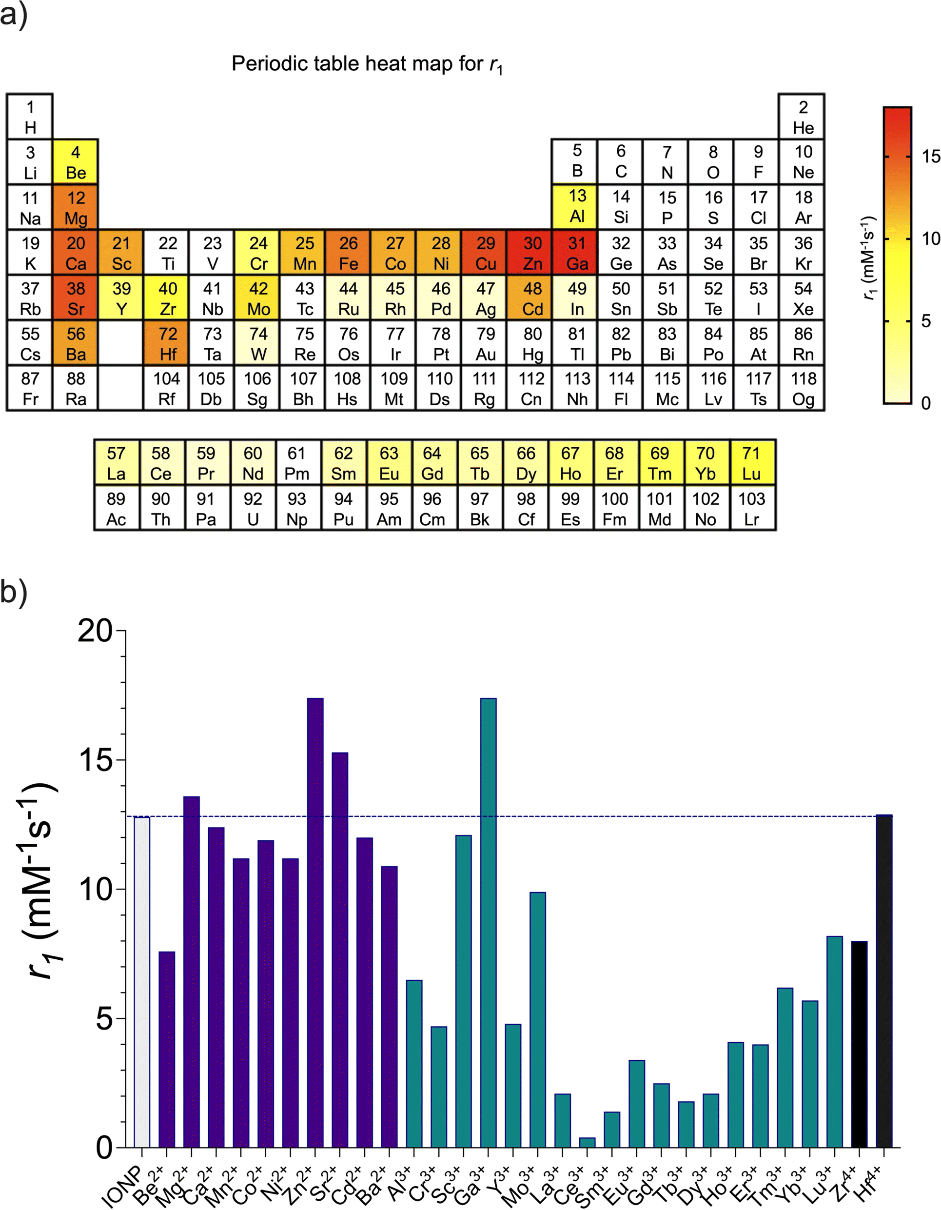 | ||
| Fig. 2 (a) Heatmap for r1 values of studied M-IONP; (b) plot of r1 values for all the metals studied, and bars are color-coded for the valence value. Measured at 1 T. | ||
Analysis of the initial screening
In the case of magnetite or maghemite, solid solutions can be formed via isomorphous substitution of Fe2+ or Fe3+ by other cations. The substitution depends on the similarity of the ionic radii and valency of the cations. Although M2+, M3+, and M4+ can enter the iron oxide structure, their uptake is usually less than 0.1 mol ratio of and depends on the synthesis method.10 M3+ cations are the most suitable, and a radius approximately 18% higher or lower can be tolerated.The introduction of doping elements changes the global magnetic moment of the nanoparticle for three reasons: (1) the nature of the cation itself determines its distribution in the crystal structure (particularly important here, in the case of spinel structures, where the distribution of cations in octahedral and tetrahedral sites defines the type of magnetic behavior); (2) the replacement of a higher magnetic moment ion, such as Fe2+ or Fe3+ (5 μB), by other ions with different magnetic moments, such as Co2+ = 3 μB, Ni2+ = 2.8 μB, Ga3+ = 3 μB, or even zero magnetic moment ions, such as Zn2+ and Mg2+, leads to a variation in MSAT; and (3) the reduction in the crystal size of the magnetic nanoparticles due to the presence of doping atoms may lead to a reduction in the nanoparticle magnetization due to magnetic moment canting effects associated with surface and internal atomic disorder.
It should be noted that the magnetic moment for magnetite arises from the balance between the distribution of ions in the Th and Oh sublattices. The metallic atoms occupy these interstitial positions, establishing two uncompensated antiparallel magnetic sublattices, where the resulting magnetic moment is M = MOh − MTh. In inverse spinel ferrites, such as magnetite, Fe2+ occupies the Oh sites, and Fe3+ ions are equally divided between the Th and Oh sites.
Here, we observed that the introduction of divalent metals such as Mn, Ni, Mg, Co, Zn, Ca, Cd, and Cu led to high MSAT values (>70 A m2 kg−1) despite the reduction in crystal size. For example, Zn2+ tends to replace iron ions at the Th sites,20 thus increasing the overall magnetic moment (98.5 A m2 kg−1) of the ferrite compared to that of IONPs (92.7 A m2 kg−1). The introduction of ions with higher magnetic moment like Mn2+, may also enhance MSAT values if they are located in Th positions. An important reduction in the MSAT value was observed when introducing diamagnetic cations such as Al3+ (66.2 A m2 kg−1) in more than 0.1 molar ratio. Therefore, although Al3+ seems to enter the cubic structure of magnetite preferentially replacing tetrahedral Fe(III),21 canting effects associated with surface and internal atomic disorder may be responsible for the MSAT reduction.
Large atoms, such as rare earth elements, have magnetic moments per atom that exceed that of Fe. However, it is difficult to incorporate them, even at the ppm level, and they tend to segregate on the surface. This has been previously observed for Gd and Bi atoms, that appear discontinuously distributed on the surface, as isolated atoms or in small clusters of oxides.22 When the atoms are incorporated, the crystal lattice deforms and particle size decreases, resulting in the decrease of the saturation magnetization.23 Rare earths ions were more inclined to replace some Fe2+ ions in the octahedral position.24 Comparing Ce3+ and La3+, Ce3+ is smaller than La3+ and the incorporation in the spinel structure is larger for Ce and therefore, MSAT is heavily reduced below 20 A m2 kg−1. In the case of Ga3+, at low contents, Ga3+ ions replace the Fe3+ ions residing in the Th site.25 This provokes a weakening of the superexchange interactions among the Th and Oh sites and a reduction in the magnetic moments of the Th sites; consequently, the net magnetization increases.
It is not easy to analyze how each variable affects the final relaxometric properties of the synthetized IONP owing to the large amount of data generated. Trying to shed some light on all these data and to find which variable is more deeply affecting the relaxometric values we carried out a multivariate analysis including the following variables: valence, ionic radii, ratio M to Fe, crystallographic peak, crystal size, hydrodynamic size, zeta potential, percentage of organic coating, saturation magnetization values and finally, r1 values. The main results of the principal component analysis are shown in Fig. 3. Fig. 3a shows the score plot of the two main principal component analyses for all variables used in the analysis. The first two principal components, PC1 and PC2, explained 67% and 25% of the variance, respectively. Furthermore, PC1 clearly differentiates metals with valence three from those with valence two. Next, we studied how all the variables correlated with each other to establish the reason for the significant change in r1 with different doping levels.
 | ||
| Fig. 3 Multivariate data analysis and main correlations of all variables used in the synthesis of different iron-oxide nanoparticles. (a) Score plot of the two principal component analyses of all variables used in the analysis. PC1 and PC2 explained 67% and 25% of the variance, respectively; (b) heatmap of the correlation matrix of the different variables. Values and the corresponding color scale are the mean of the side-by-side replicates of the Pearson (r) correlation coefficients; (c) plot and linear regression between MSAT and r1 of iron oxide nanoparticles (colors are the same as those indicated in panel (a)); (d) Box plot of MSATversus the valence of the cation added to IONP. Data are presented as mean ± SD. | ||
Fig. 3b shows a heatmap of all variables, with Pearson (r) correlation coefficients in each box. Several conclusions can be drawn from the graph. For example, variables such as the ionic radii, ratio of M to Fe (for the studied sample), and crystal size did not show an important correlation with r1. However, there are several correlations that help to understand the behavior of these samples. For example, there is a positive correlation between the size determined by DLS and r1 values; that is, the higher the hydrodynamic size, the higher the r1. This may seem contradictory, but is explained by the negative correlation between the hydrodynamic size and the amount of organic coating for the studied samples. In other words, for these samples, the lower the amount of organic coating, the larger is the hydrodynamic size and r1 value. This result is in agreement with what is known about this type of nanomaterials. In 2017, we demonstrated that increasing the organic coating changed the behavior from optimal for T1 to optimal for T2,7 these results further confirmed this. Related to this is the large and negative (−0.71) correlation between the percentage of organic material and r1 value. However, according to this analysis, the major contributor to the change in r1 was the saturation magnetization data. A strong positive correlation (0.89) was observed, indicating that the higher the magnetization value, the larger r1. Fig. 3c shows the linear fit of r1 values versus magnetization. In addition to the clear correlation, the data are color-coded for the valence of each ion. This representation shows how metals with valence 3+ are in the lower part of the graph, with low values for MSAT and r1, while most of the 2+ metals are in the upper part of the graph, with large MSAT and r1 values. A notable exception to this behavior is Ga3+, which shows a very large r1 value, second only to Zn2+. The difference between the MSAT values according to the valence of the metal was statistically significant, again showing much higher values for M2+ than M3+ (Fig. 3d).
Ga and Zn doped IONP
Doping extremely small iron oxide nanoparticles with 30 different metals produced a large variation in the r1 values. It is clear that doping IONP with Zn2+ or Ga3+ results in the largest increase in r1. The different syntheses doping with 1.5 mM of these metals rendered equal r1 values of 17.4 ± 0.6 mM−1 s−1 for Zn2+ and 17.4 ± 0.8 mM−1 s−1 for Ga3+ (units given as mM of all metals involved). Considering these results, we thought it would be interesting to explore what would happen if we simultaneously used these two metals to produce Ga- and Zn-doped iron oxide nanomaterials in an attempt to find a synergistic response for r1. For this reason, we used the same synthetic protocol as for the other 30 nanomaterials used to produce GaZn-IONP. We explored different Zn![[thin space (1/6-em)]](https://www.rsc.org/images/entities/char_2009.gif) :Fe and Ga:Fe molar ratios and achieved the best results with molar ratios of 0.02 for Zn2+ and 0.01 for Ga3+. GaZn-IONP were synthesized as very small homogenous spherical particles, as observed by electron microscopy (Fig. 4), in these images no difference is observed between Zn-IONP, Ga-IONP and GaZn-IONP. Core sizes were measured in TEM images with the following values: 3.7 ± 0.8 nm for Ga-IONP; 3.6 ± 0.4 nm for Zn-IONP and 3.8 ± 0.4 nm for GaZn-IONP. Thermogravimetric, infrared spectroscopy, XRD, and magnetization measurements showed that both nanomaterials, GaZn-IONP and IONP, were almost identical in terms of surface composition, crystal structure, and magnetic behavior (Fig. 5a–d).
:Fe and Ga:Fe molar ratios and achieved the best results with molar ratios of 0.02 for Zn2+ and 0.01 for Ga3+. GaZn-IONP were synthesized as very small homogenous spherical particles, as observed by electron microscopy (Fig. 4), in these images no difference is observed between Zn-IONP, Ga-IONP and GaZn-IONP. Core sizes were measured in TEM images with the following values: 3.7 ± 0.8 nm for Ga-IONP; 3.6 ± 0.4 nm for Zn-IONP and 3.8 ± 0.4 nm for GaZn-IONP. Thermogravimetric, infrared spectroscopy, XRD, and magnetization measurements showed that both nanomaterials, GaZn-IONP and IONP, were almost identical in terms of surface composition, crystal structure, and magnetic behavior (Fig. 5a–d).
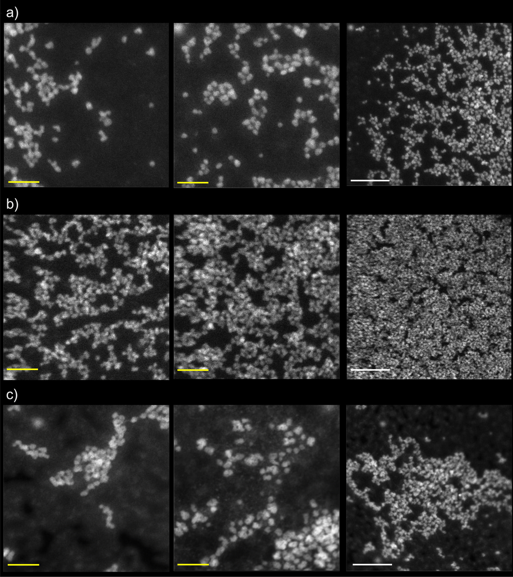 | ||
| Fig. 4 STEM-HAADF images of (a) Ga-IONP; (b) Zn-IONP and (c) GaZn-IONP (yellow bar is 20 nm, white bar is 50 nm). | ||
 | ||
| Fig. 5 Physicochemical characterization of GaZn-IONP and comparison with IONP using (a) thermogravimetric analysis; (b) FTIR spectroscopy; (c) XRD spectroscopy; (d) magnetization curves; (e) temperature dependence of AC magnetic susceptibility. (f) Plot and linear fitting of 1/T1versus the sum of iron, gallium and zinc concentrations; (g) r1 values for five different syntheses of IONP, ZnIONP, GaIONP and GaZn-IONP and (h) EDS analysis of an area containing a large number of particles showing the presence of iron and oxygen as part of the composition of the material. The elemental maps show the presence of gallium and zinc, although in much smaller amount in the same areas where the iron and oxygen are detected, homogeneously distributed. | ||
We further studied the magnetic behavior of GaZn-IONP by magnetic susceptibility measurements. Both the in-phase (χ′) and out-of-phase (χ′′) components of the AC magnetic susceptibility were recorded as a function of temperature for the IONP and GaZn-IONP samples. In both cases, a single maximum in the χ′(T) and χ′′ (T) plots was observed for each material (Fig. 5e and supp. Info). The fact that, for each particle, the χ′′(T) maximum is located at a slightly lower temperature than the χ′(T) indicated a relaxation phenomenon typical of magnetic nanoparticles. Analysis of the χ′′(T) maximum is especially relevant in the study of magnetic nanoparticles. The location in temperature of the out-of-phase susceptibility maximum depends on several parameters including the particle size distribution, its composition and degree of dipolar interactions and therefore, can inform about differences among the particles. In this case, two main parameters could affect the χ′′(T) profile. Particles have slightly different average particle size, being 38.7 Å for the GaZn-IONP and 34.1 Å for the IOPN. If only size is considered, the location of the out-of-phase susceptibility maxima should be at higher temperatures for the GaZn-IONP, as it has been reported in the past that small differences in average particle size can be tracked by this technique, leading to maxima located at higher temperatures for the larger particles in very similar materials.7 Interestingly, our results showed a maximum located at lower temperatures for the materials with larger particle sizes (Fig. 5e). This result is a clear indication of the effect of the Ga and Zn doping on the effective anisotropy constant of the material, that mostly depends on the chemical composition, and that leads to the location of the χ′′(T) maxima at lower temperature for the particles with the bigger size (GaZn-IONP). This effect has been recently reported for similar particles, in which a higher degree of Mn doping leads to maxima at lower temperatures.26,27 These small differences explain the values measured in the final relaxometric study (Fig. 5f and g). Relaxometry of GaZn-IONP provided a value of r1 equal to 19.6 ± 0.8 mM−1 s−1 and r2 of 41.9 ± 1.8 mM−1 s−1, thus an r2/r1 ratio of 2.1 (units given as mM of all metals involved). Fig. 5g shows the r1 values for IONP, Ga-IONP, Zn-IONP and GaZn-IONP where the evolution of this value with the different core composition is observed. These results confirmed our hypothesis that the combination of Zn2+ and Ga3+ could improve the already good values for the single doped nanoparticles. EDS was also used to check for the presence of Ga and Zn in the core of the IONP (Fig. 5h and S7†). The presence of these metals, together with Fe, can be observed even when considering the small amounts in which they are incorporated.
In vivo MRI using GaZn-IONP
Encouraged by the physicochemical characterization of the GaZn-IONP, we decided to test their performance as T1-weighted MRI probes. These experiments are particularly important because of the well-known reduction in r1 for IONP when large magnetic fields are used. To demonstrate that the large increment in r1 at 1 T also has a significant impact on the in vivo imaging of small animals, often performed at very large magnetic fields, we designed two complementary experiments. For this purpose, we carried out two different experiments: magnetic resonance angiography in healthy mice and glioblastoma diagnosis in a mouse model.GaZn-IONP as MRI probe
GaZn-IONP were tested as magnetic resonance angiography (MRA) probe in two different concentrations, the standard concentration used for most Gd-based probes (0.1 mmol Fe–Ga–Zn per kg) and two less concentrated samples (0.05 mmol Fe–Ga–Zn per kg and 0.01 mmol Fe–Ga–Zn per kg). The main results of the MRA experiments are shown in Fig. 6. In this figure, we can see the strong positive signal provided by the GaZn-IONP at a high field (7 T). The heart and aorta can be observed in detail using a concentration half of the typical concentration used with Gd 15 min after intravenous injection (Fig. 6a). One of the problems when using small Gd chelates is that they rapidly extravasate; therefore, we wanted to test GaZn-IONP at low concentrations for longer periods of time. Fig. 6b shows the signal 120 min after intravenous injection. The signal was reduced compared with that obtained after 15 min, but it was still clearly possible to see the aorta in detail. Finally, we wanted to further push the experimental conditions and carried out an MRA experiment in three animals using a concentration 10 times lower than the usual concentration of Gd (Fig. 6c). Even under these conditions, it was possible to observe the aorta 15 min after the intravenous injection. Owing to the positive contrast provided by the GaZn-IONP, it is possible to see several anatomical details in the mouse; for example, we can appreciate the circulation of the nanoparticles in the kidneys (Fig. 6d), the aorta bifurcation, and the kidney (Fig. 6e), and even at 0.01 mmol Fe–Ga–Zn per kg, it is possible to clearly see the positive signal in the heart and aorta (Fig. 6f). | ||
| Fig. 6 Magnetic resonance angiography, at 7 T, of the aortas of healthy mice. (a) 15 minutes after the injection of 0.05 mmol Fe–Ga–Zn per kg of GaZn-IONP; (b) 120 minutes after the injection of 0.05 mmol Fe–Ga–Zn per kg of GaZn-IONP; (c) 15 minutes after the injection of 0.01 mmol Fe–Ga–Zn per kg of GaZn-IONP; (d) anatomic detail of one kidney after the injection of 0.1 mmol Fe–Ga–Zn per kg of GaZn-IONP; (e) anatomic detail of one kidney and the aorta after the injection of 0.1 mmol Fe–Ga–Zn per kg of GaZn-IONP and (f) anatomic detail of one aorta and heart after the injection of 0.01 mmol Fe–Ga–Zn per kg of GaZn-IONP. | ||
MRA is a typical experiment to demonstrate whether an imaging probe provides positive contrast in MRI. Because of the characteristics of such experiments, that is, the rapid dilution of the nanoparticles in the bloodstream, conditions are ideal to avoid aggregation of the nanoparticles, which could lead to an increase in T2 effects, making it more difficult to obtain a good T1 signal in vivo. Considering the optimal results obtained in MRA, even at very low concentrations, we wanted to test GaZn-IONP in a more challenging scenario.
Glioblastoma is a highly malignant and aggressive form of brain cancer that originates from glial cells in the brain, which support and nourish nerve cells. It is known for its rapid growth and infiltrative nature, which makes its diagnosis and treatment challenging. Glioblastoma often leads to severe neurological symptoms and has a grim prognosis, with a median survival of approximately 12–15 months even with aggressive treatment. The diagnosis of glioblastoma is critically important for treatment planning, prognosis, and development of personalized care for patients. Therefore, we chose a glioblastoma mouse model to test the performance of GaZn-IONP. A key issue when developing diagnostic or treatment approaches for GBM is the blood–brain barrier (BBB), which restricts the uptake of most compounds, thus limiting the diagnostic and therapeutic options. When GBM and other tumors develop cancer cells that displace endothelial cells from the BBB, this breaks down the barrier, altering passive and active transport and producing the blood tumor barrier (BTB). Even if this barrier is more permeable than the BBB, its permeability is very heterogeneous, and it is not clear beforehand how the therapeutic or diagnostic compound is affected. Nanoparticles are increasingly being used for brain diseases but, even for nanoparticles as small as our GaZn-IONP it was not clear whether they could cross the barrier and efficiently accumulate in the tumor.28
This experiment allowed us to assess two questions: Would the nanoparticles cross the affected BBB-BTB? And, considering such a large magnetic field and the possible accumulation of nanoparticles, would they still provide a clear positive signal in the tumor?
To answer these questions, we used an orthotopic glioma model generated in three NOD-SCID mice at 8–10 weeks and performed MRI after tumor development. Tumor development was monitored using T2-weighted MRI twice a week. Three weeks after tumor generation, mice were subjected to nanoparticle experiments. We intravenously injected 0.06 mmol Fe–Ga–Zn per kg and imaged the brain 90 min post-injection. No toxicity was observed in mice, in agreement with previous studies with this type of nanomaterial. The results showed different images for the developed glioblastoma in the brain; baseline images were recorded, and the T1 signal was measured after the injection of nanoparticles (Fig. 7a and S8–S10†). Images show a brightening of the tumor area after the injection of GaZn-IONP, including what it seems the inner part of the tumor. An increase in the relative contrast enhancement (RCE) of the tumor relative to the contralateral-healthy brain was also observed in T1W images 90 min after nanoparticle injection (44.30 ± 4.56%) compared to the pre-injection RCE (0.93 ± 0.97%, Fig. 7b). To further demonstrate the presence of nanoparticles in the lesion, we performed consecutive T1 and T2 imaging. The results are shown in Fig. 7c, demonstrating the positive signal in the tumor and how the same areas turned black owing to the negative contrast provided by the nanoparticles, confirming that the signals we observed came from the uptake of GaZn-IONP in the tumor. These changes were measured using the RCE (Fig. 7d). The results confirm the increase in the brightness of the T1 signal, which is reduced when switching to T2-weighted imaging. T2W images acquired 90 min after nanoparticle injection showed a decrease in RCE of the tumor relative to the contralateral (−49.67 ± 15.49%) compared to the pre-injection RCE (12.68 ± 4.54%).
 | ||
| Fig. 7 MRI, at 7 T, of the glioblastoma mouse model. (a) T1 images for baseline and 90 min after the injection of 0.06 mmol Fe–Ga–Zn per kg of GaZn-IONP; (b) relative contrast enhancement for images in (a); (c) T1- and T2-weighted MRI for glioblastoma model before and after the injection of GaZn-IONP, and (d) relative contrast enhancement for images in (c). | ||
Conclusions
We carried out a thorough investigation into the impact of core doping nanoparticles, optimized for enhanced contrast in MRI, on the magnetic and relaxometric characteristics of these probes. We synthesized 30 different nanomaterials and found that the r1 value improved in four of them. Using multivariate analysis, we evaluated the contribution of various factors to the relaxometric properties of the nanoparticles. By combining the two metals with the greatest effect, Ga and Zn, we were able to increase the r1 value to one of the largest reported values. The enhanced probes were then tested in vivo, where they provided clear positive signals at concentrations ten times smaller than those clinically approved for these types of probes. Finally, we demonstrated that GaZn-IONP can passively accumulate in a glioblastoma model, highlighting the tissue on MRI and opening the possibility of new diagnosis and treatment approaches for this disease.Materials and methods
Synthesis of M-IONP
The synthesis was performed in a silicone bath that was preheated to 120 °C and using a high-pressure microwave vial closed with a cap and a silicon septum. FeCl3·6H2O (75 mg, 0.27 mmol), sodium citrate tribasic dihydrate (80 mg, 0.27 mmol), and the corresponding metal salt were dissolved in water (Milli-Q grade, 9 ml) in a 20 ml reaction vial. The solution was placed inside a silicone oil bath, and after reaching the reaction temperature (120 °C), hydrazine monohydrate was quickly added (1 ml) through the septum. The reaction was stirred for 45 min and rapidly stopped by placing the mixture in an ice/water bath. Purification was performed by size-exclusion chromatography using pre-packed Sephadex G-25 M (PD10) columns.Magnetic behavior of M-IONP
T1 and T2 relaxation properties in nuclear magnetic resonance (NMR).The effect of the M-IONP samples on the longitudinal (spin-lattice. T1) and transverse (spin–spin. T2) relaxation times were measured by NMR using a static magnetic field of 1 T generated with a Magritek Spinsolve 43 MHz benchtop spectrometer. Four different dilutions (0.1–4.0 mM) were measured for each sample, depending on the initial concentration and a blank (MilliQ water) at 37 °C. The r1 and r2 values (factors used to evaluate the efficiency of a sample as a contrast agent) were obtained as the slope resulting from the linear fit of the 1/T1/2 (s−1) relaxation time versus the Fe + M concentration (mM) determined by ICP-MS.
Magnetic characterization
The field-dependent magnetization of the M-IONP was studied using a vibrating sample magnetometer (VSM) MLVSM9 MagLab 9T (Oxford Instruments). The sample mass was corrected to a magnetic source mass by removing the organic/moisture component. The freeze-dried powder was compacted in a non-magnetic capsule and measured at 290 K within a field range of – 5 to 5 T. The temperature dependence of the AC magnetic susceptibility was recorded using an MPMS-XL (Quantum Design) SQUID magnetometer between 2 and 100 K, using an AC magnetic field with an amplitude of 4.1 Oe (326.3 A m−1) and a frequency of 11 Hz. For these measurements, the samples were prepared by placing a known volume of the particle suspension on a cotton piece and allowing it to dry. The cotton pieces were then transferred into individual gelatin capsules for magnetic characterization.MRI acquisition
The M-IONP were selected for their potential use as positive contrast agents and their behavior at higher magnetic fields was evaluated.MRA of healthy mice
In vivo MRA imaging was performed on 24 C57BL/6JRj male mice with a body weight of 30 g divided into six groups (n = 4). Prior to administration, MRA scans were performed as part of a control imaging experiment. Subsequently, different concentrations (0.01, 0.05 and 0.1 mmol kg−1) of either (i) Gadovist or (ii) GaZn-IONP were intravenously administered (mmol of Gd or mmol of Fe–Ga–Zn). Post-administration images were acquired at time intervals of 15, 45, and 120 minutes. Anesthesia was induced using 4% isoflurane in 70% oxygen and 30% nitrogen, and anesthesia was maintained with 1–2% isoflurane during imaging acquisition. To ensure the well-being of the mice, anal temperature and respiration (through a respiratory pad) were continuously monitored throughout the experiment using an MRI compatible system interfaced to a Monitoring and Gating Model 1030 (SA Instrument, Stony Brook, NY, USA).MRA experiments were conducted using a 7 Tesla Bruker Biospec 70/30 USR MRI system (Bruker Biospin GmbH, Ettlingen, Germany) interfaced with an AVANCE III console. A BGA12 imaging gradient system (maximum gradient strength 400 mT m−1) with a 40 mm diameter quadrature volume resonator (Bruker Biospin GmbH, Ettlingen, Germany) was utilized for MRA data acquisition. Anatomical images of the body were obtained using a 3D FLASH flow-compensated sequence using the following parameters: TE/TR = 1.94/21 ms. Flip angle 60°, 2 averages, acquisition matrix 256 × 192 × 128, a Field of View of 55 × 38 × 25.60 mm, with a total acquisition time of 17 minutes.
Animal experiments were conducted in the CIC biomaGUNE accredited animal facility, which holds full accreditation from AAALAC. Animal procedures were approved by our Institutional Animal Care and Committee and local authorities (Diputación Foral de Guipúzcoa. Spain; protocol ID: PRO-AE-SS-225).
In vivo glioma model
Authenticated glioma C6 cells from the American Type Culture Collection (number CCL-107, Manassas, VA, USA) were cultured in DMEM supplemented with 10% fetal bovine serum and antibiotics (10% amphotericin, 100 UI per ml penicillin, 0.03 mg per ml gentamicin, and 0.1 mg per ml streptomycin). The cells were maintained in an incubator at 37 °C and 5% CO2 until they reached confluence, detached, and counted to generate the glioma model.An orthotopic glioma model was generated in three NOD-SCID mice of 8–10 weeks of age, as previously reported.29 Briefly, mice were placed in a stereotaxic device where anesthesia was maintained through a nose mask (1–1.5% isoflurane/O2), and the eyes were covered with Vaseline to prevent them from drying out. Then, a midline incision on the skull was made using a scalpel, and a burr hole was performed 0.23 mm right of the bregma using a 25G needle. Then, 105 C6 cells in 10 μL of DMEM with 30% Matrigel were injected to a depth of 0.33 mm in the right caudate nucleus with a Hamilton syringe. After 5 min, the syringe was carefully removed, the hole was sealed with bone wax, and the scalp sutured. The animals were injected subcutaneously with buprenorphine for analgesia 30 min before the procedure and for the following 2 days (0.1 mg kg−1).
MRI studies of glioma model
MRI studies were performed on a horizontal 7.0-Tesla Bruker Biospec® system (Bruker Medical GmbH, Ettlingen, Germany) using a 40 mm transmitter coil with a 23 mm mouse brain surface coil as the receiver. MR images were acquired using ParaVision 6.0.1 software operating in a Linux environment. Animals were anesthetized as described in the tumor generation protocol, and anesthesia was maintained through a nose mask throughout the MRI experiment. Body temperature was maintained at 37 °C using a heated waterbed, and respiratory rate was monitored during the MRI study.Tumor development was monitored using T2-weighted MRI twice a week. Three weeks after tumor generation, mice were subjected to nanoparticle experiments. First, a baseline study was performed prior to nanoparticle injection. acquiring two types of MR images in an axial orientation with 14 slices of 1 mm slice thickness, a matrix size of 256 × 256 s, and a field of view (FOV) of 23 × 23 mm2, corresponding to an in-plane resolution of 90 × 90 μm2:
-T2 weighted (T2W) images were obtained using a rapid acquisition with relaxation enhancement (RARE) sequence, with a repetition time (TR) = 2500 ms, effective echo time (TE eff) = 26 ms, RARE factor = 8, number of averages (Av) = 4 and total acquisition time (TAT) = 4 min.
-T1 weighted (T1W) images using a multi-slice multi-echo sequence (MSME) with TR = 300 ms, echo time TE eff = 10 ms, Av = 3, TAT = 3 min, and 50 s.
The mice were then intravenously injected with 200 μL ([Fe] = 1.2 mg ml−1, [Ga] = 0.03 mg ml−1 and [Zn] = 0.03 mg ml−1) of the nanoparticle preparation and 90 min after injection, the animals were again examined by MRI, using the same set of images acquired in the baseline study.
Images were analyzed using ImageJ (National Institute of Health, NIH) by manually selecting two regions of interest (ROIs) with a size of approximately 20 pixels in a representative slice. One ROI was selected within the tumor region with active contrast uptake, and the other within the contralateral-healthy brain. The percentage of relative contrast enhancement (RCE) of the signal intensity (SI) of the tumor ROI versus the SI of the contralateral ROI was calculated at baseline (pre-nanoparticle injection) and 90 min post-injection MRI studies for T1W and T2W images, respectively.
Ethics approval statement
All animal experiments have been conducted after approval of Comunidad de Madrid regional government authorities.Data availability
The data that support the findings of this study are available from the corresponding author upon reasonable request.Author contributions
The manuscript was written through contributions of all authors. All authors have given approval to the final version of the manuscript.Conflicts of interest
The authors declare no conflict of interest.Acknowledgements
This study was supported by a grant for predoctoral contracts for the training of PhD students from the Spanish Ministry of Science and Innovation (grant number PRE2020-091870), associated with the National Plan project PID2019-104059RB-100. We acknowledge funding from the Spanish Ministry of Science and Innovation (PID2021-123238OB-100, PDC2022-133493-100, RED2022-134299-T), La Caixa Foundation (Health Research Call 2020: HR20-00075), the Basque Government, R&D Projects in Health (Grant no. 2022333041) and Comunidad de Madrid (P2022/BMD-7333). Conexión Nanomedicina CSIC.Notes and references
- R. K. Kawassaki, M. Romano, M. Klimuk Uchiyama, R. M. Cardoso, M. S. Baptista, S. H. P. Farsky, K. T. Chaim, R. R. Guimarães and K. Araki, Nano Lett., 2023, 23, 5497 CrossRef CAS PubMed.
- I. Fernández-Barahona, M. Muñoz-Hernando, J. Ruiz-Cabello, F. Herranz and J. Pellico, Inorganics, 2020, 8, 28 CrossRef.
- Z. Zhao, M. Li, J. Zeng, L. Huo, K. Liu, R. Wei, K. Ni and J. Gao, Bioact. Mater., 2022, 12, 214 CAS.
- W. Xie, Y. Gan, Y. Zhang, P. Wang, J. Zhang, J. Qian, G. Zhang and Z. Wu, J. Mater. Chem. B, 2022, 10, 1039 Search PubMed.
- M. Porru, M. del P. Morales, A. Gallo-Cordova, A. Espinosa, M. Moros, F. Brero, M. Mariani, A. Lascialfari and J. G. Ovejero, Nanomaterials, 2022, 12, 3304 CrossRef CAS PubMed.
- C. Lu, X. Xu, T. Zhang, Z. Wang and Y. Chai, J. Mater. Chem. B, 2022, 10, 1623 RSC.
- J. Pellico, J. Ruiz-Cabello, I. Fernández-Barahona, L. Gutiérrez, A. V. Lechuga-Vieco, J. A. Enríquez, M. P. P. Morales and F. Herranz, Langmuir, 2017, 33, 10239 CrossRef CAS PubMed.
- I. Fernández-Barahona, L. Gutiérrez, S. Veintemillas-Verdaguer, J. Pellico, M. del P. Morales, M. Catala, M. A. del Pozo, J. Ruiz-Cabello and F. Herranz, ACS Omega, 2019, 4, 2719 CrossRef PubMed.
- I. Fernández-Barahona, L. Gutiérrez, S. Veintemillas-Verdaguer, J. Pellico, M. del P. Morales, M. Catala, M. A. del Pozo, J. Ruiz-Cabello and F. Herranz, ACS Omega, 2019, 4, 2719 CrossRef PubMed.
- R. M. Cornell and U. Schwertmann, The Iron Oxides: Structure, Properties, Reactions, Occurences and Uses, Wiley, 2003 Search PubMed.
- W. Wu, Z. Wu, T. Yu, C. Jiang and W.-S. Kim, Sci. Technol. Adv. Mater., 2015, 16, 023501 CrossRef PubMed.
- A. L. Patterson, Phys. Rev., 1939, 56, 978 CrossRef CAS.
- D. Maity and D. C. Agrawal, J. Magn. Magn. Mater., 2007, 308, 46 CrossRef CAS.
- S. Alibeigi and M. R. Vaezi, Chem. Eng. Technol., 2008, 31, 1591 CrossRef CAS.
- J. Pellico, I. Fernández-Barahona, J. Ruiz-Cabello, L. Gutiérrez, M. Muñoz-Hernando, M. J. Sánchez-Guisado, I. Aiestaran-Zelaia, L. Martínez-Parra, I. Rodríguez, J. Bentzon and F. Herranz, ACS Appl. Mater. Interfaces, 2021, 13, 45279 CrossRef CAS PubMed.
- J. M. Adrover, J. Pellico, I. Fernández-Barahona, S. Martín-Salamanca, J. Ruiz-Cabello, A. Hidalgo and F. Herranz, Nanoscale, 2020, 12, 22978 RSC.
- J. Pellico, I. Fernández-Barahona, M. Benito, Á. Gaitán-Simón, L. Gutiérrez, J. Ruiz-Cabello and F. Herranz, Nanomed.: Nanotechnol. Biol. Med., 2019, 17, 26 CrossRef CAS PubMed.
- J. Pellico, A. V. Lechuga-Vieco, E. Almarza, A. Hidalgo, C. Mesa-Nuñez, I. Fernández-Barahona, J. A. Quintana, J. Bueren, J. A. Enríquez, J. Ruiz-Cabello and F. Herranz, Sci. Rep., 2017, 7, 13242 CrossRef PubMed.
- T. Vangijzegem, D. Stanicki, S. Boutry, Q. Paternoster, L. Vander Elst, R. N. Muller and S. Laurent, Nanotechnology, 2018, 29, 265103 CrossRef CAS PubMed.
- A. Kolhatkar, A. Jamison, D. Litvinov, R. Willson and T. Lee, Int. J. Mol. Sci., 2013, 14, 15977 CrossRef PubMed.
- U. Schwertmann, Clays Clay Miner., 1990, 38, 196 CrossRef CAS.
- M. Andrés-Vergés, M. Del Puerto Morales, S. Veintemillas-Verdaguer, F. J. Palomares and C. J. Serna, Chem. Mater., 2012, 24, 319 CrossRef.
- X. Zheng, J. Tan, Q. Wang, C. Gao, X. Yu, W. Xie, Y. Yang, Y. Wang and C. Jin, J. Alloys Compd., 2023, 935, 168120 CrossRef CAS.
- M. Zeng, K. Thummavichai, W. Chen, G. Liu, Z. Li, X. Chen, C. Feng, Y. Li, N. Wang and Y. Zhu, RSC Adv., 2021, 11, 37246 RSC.
- M. A. Almessiere, Y. Slimani, S. Ali, A. Baykal, R. J. Balasamy, S. Guner, İ. A. Auwal, A. V. Trukhanov, S. V. Trukhanov and A. Manikandan, Nanomaterials, 2022, 12, 2872 CrossRef CAS.
- S. Carregal-Romero, A. B. Miguel-Coello, L. Martínez-Parra, Y. Martí-Mateo, P. Hernansanz-Agustín, Y. Fernández-Afonso, S. Plaza-García, L. Gutiérrez, M. D. M. Muñoz-Hernández, J. Carrillo-Romero, M. Piñol-Cancer, P. Lecante, Z. Blasco-Iturri, L. Fadón, A. C. Almansa-García, M. Möller, D. Otaegui, J. A. Enríquez, H. Groult and J. Ruíz-Cabello, Small, 2022, 18, 2106570 CrossRef CAS PubMed.
- D. García-Soriano, R. Amaro, N. Lafuente-Gómez, P. Milán-Rois, Á. Somoza, C. Navío, F. Herranz, L. Gutiérrez and G. Salas, J. Colloid Interface Sci., 2020, 578, 510 CrossRef PubMed.
- D. Ruiz-Molina, X. Mao, P. Alfonso-Triguero, J. Lorenzo, J. Bruna, V. J. Yuste, A. P. Candiota and F. Novio, Cancers, 2022, 14, 4960 CrossRef CAS PubMed.
- N. Arias-Ramos, L. E. Ibarra, M. Serrano-Torres, B. Yagüe, M. D. Caverzán, C. A. Chesta, R. E. Palacios and P. López-Larrubia, Pharmaceutics, 2021, 13, 1258 CrossRef CAS PubMed.
Footnote |
| † Electronic supplementary information (ESI) available. See DOI: https://doi.org/10.1039/d4sc01069h |
| This journal is © The Royal Society of Chemistry 2024 |