DOI:
10.1039/D3SC05552C
(Edge Article)
Chem. Sci., 2024,
15, 1449-1471
CarsiDock: a deep learning paradigm for accurate protein–ligand docking and screening based on large-scale pre-training†
Received
19th October 2023
, Accepted 18th December 2023
First published on 19th December 2023
Abstract
The expertise accumulated in deep neural network-based structure prediction has been widely transferred to the field of protein–ligand binding pose prediction, thus leading to the emergence of a variety of deep learning-guided docking models for predicting protein–ligand binding poses without relying on heavy sampling. However, their prediction accuracy and applicability are still far from satisfactory, partially due to the lack of protein–ligand binding complex data. To this end, we create a large-scale complex dataset containing ∼9 M protein–ligand docking complexes for pre-training, and propose CarsiDock, the first deep learning-guided docking approach that leverages pre-training of millions of predicted protein–ligand complexes. CarsiDock contains two main stages, i.e., a deep learning model for the prediction of protein–ligand atomic distance matrices, and a translation, rotation and torsion-guided geometry optimization procedure to reconstruct the matrices into a credible binding pose. The pre-training and multiple innovative architectural designs facilitate the dramatically improved docking accuracy of our approach over the baselines in terms of multiple docking scenarios, thereby contributing to its outstanding early recognition performance in several retrospective virtual screening campaigns. Further explorations demonstrate that CarsiDock can not only guarantee the topological reliability of the binding poses but also successfully reproduce the crucial interactions in crystalized structures, highlighting its superior applicability.
Introduction
Accurate characterization of the protein–ligand recognition process is of central importance for the understanding of various biological processes, e.g., enzyme catalysis, signaling transduction and drug binding. Experimental techniques, such as X-ray diffraction,1 nuclear magnetic resonance (NMR) crystallography2 and cryogenic electron microscopy (cryo-EM),3 can be used to decode the structure information of protein–ligand interactions, but they usually suffer from high cost and poor accessibility. As an alternative to experimental measurement, computational docking approaches, e.g., DOCK,4,5 AutoDock,6 AutoDock Vina,7,8 GOLD9 and Glide,10,11 have been successively developed and contribute enormously to structure-based drug design.12,13
A typical molecular docking protocol generally consists of two major stages, i.e., sampling and scoring. The former aims to sample as many binding poses of a molecule as possible in the desired binding pocket, and the latter tends to assess the binding strength of each pose using a predefined scoring function (SF). To reduce the searching space, many heuristic algorithms have been employed for pose sampling, e.g., genetic algorithms used by AutoDock and GOLD and the ant colony algorithm used by PLANTS.14 Another remarkable advance worth mentioning is the introduction of graphics processing units (GPU) into docking calculation for acceleration, represented by AutoDock-GPU15 and Vina-GPU.16 However, though the searching efficiency has been dramatically enhanced, their accuracy is still limited due to the difficulty of complete convergence in limited searching steps. On the other hand, the SFs employed in traditional docking programs are primarily physics-based or empirical approaches, which assume an additive formulated hypothesis to describe the relationships between binding affinities and various interaction features such as van der Waals interactions and electrostatic interactions. The binding affinities given by these SFs in many cases cannot well rank the binding poses, suggesting that their reliability still needs improvement.17,18
The rapid development of machine learning (ML) and artificial intelligence (AI) in the past few years has brought in several promising directions in the molecular docking field. One of the most pioneering outcomes is ML-based SFs (MLSFs), which rely on the powerful non-linear fitting capability of AI algorithms to capture the intrinsic interactions between ligands and their targets.19–22 This type of approach could achieve remarkably superior performance compared to classical methods on several retrospective benchmarks, but most of them are just tailored for rescoring, implying that traditional docking programs are still needed to generate the binding poses in advance. Two exceptions are Gnina23 and DeepDock,24 which have embedded MLSFs with traditional heuristic algorithms as an integrated protocol for both sampling and scoring; however, they may be still faced with the limitations mentioned above. Another hot direction is ML-based docking score predictors, which are trained on a subset of a compound library and then employed to predict the docking scores for the remaining library members.25–27 This strategy could significantly improve the screening efficiency for ultra-large chemical libraries, but from another point of view, their prediction accuracy can never exceed the ones without the use of ML.
Thanks to the revolutionary progress achieved by AlphaFold2 (ref. 28) for structural biology, a series of deep learning (DL)-guided docking models for predicting protein–ligand binding poses without depending on heavy sampling have been successively proposed.29–36 Among them, EquiBind29 is a pioneer method, which relies on an attention-based key-point alignment mechanism to directly predict the coordinates of the binding poses. Successive attempts include TankBind,30 E3Bind31 and DiffDock.32 These models could generally outperform traditional methods in the scenario of blind docking, where the binding pocket of the target is unknown, but considering that almost all the classical baseline docking programs are not designed for this scenario, the comparison is apparently unfair. In contrast, the scenarios with known binding sites shall be more common in real-world applications, and even if the pockets are unknown, they can also be easily detected by some external pocket predictors such as FPocket37 and P2Rank.38 Of course, there are also a few pocket-centralized models reported very recently, such as MedusaGraph,33 LigPose,34 EDM-Dock35 and Uni-Mol.36 MedusaGraph is more like a binding pose optimization model, which feeds the docking poses as inputs and then leverages graph neural networks (GNNs) to optimize the poses. LigPose relies on equivariant graph neural network (EGNN) to directly update the coordinates of the ligand, while EDM-Dock first converts the binding pose into an intermolecular Euclidean distance matrix and then reconstructs the distance map of the ligand pose. These models have achieved substantial improvements compared with traditional approaches, but they just utilize the limited crystalized complex structures for model training. Uni-Mol is a universal molecular representation learning framework and one of its downstream tasks is to predict protein–ligand binding poses. It creatively introduces two large-scale pre-training models for the independent representation learning of ligands and protein pockets, but this setting inevitably ignores the potential intermolecular relationships in a bound state.
In this study, we propose CarsiDock, to the best of our knowledge, the first DL-guided docking approach that leverages large-scale pre-training of millions of docking complexes for protein–ligand binding pose generation. CarsiDock consists of two major steps, i.e., using a DL model to predict the protein–ligand atomic distance matrices and obtain a distance–aware mixture density model critical for binding pose ranking, and then reconstructing the final binding pose from the predicted distance map by updating the translations, rotations and torsion angles of the initial binding poses with the hierarchical guidance of three elaborately designed scoring schemes. To improve the model performance, we create a large-scale complex dataset containing ∼9 M protein–ligand docking complexes for pre-training, followed by fine-tuning on a well-recognized dataset composed of just the crystalized complex structures. In addition to the above innovations, we further incorporate the triangle self-attention mechanism to enhance the learning of intermolecular interactions, a customized self-distillation pipeline to improve model training, and two data augmentation strategies to enhance model generalization. The integrated use of these strategies enables our approach to perform competitively in terms of both the docking accuracy and screening capability on several widely recognized benchmarks. Further investigations indicate that CarsiDock can not only maintain the topological reliability of binding poses but also successfully recover the key interactions in crystalized structures, highlighting the excellent applicability of the approach.
Results and discussion
Overview of CarsiDock
Fig. 1A depicts the overview of CarsiDock, which consists of a DL model to predict the protein–ligand atomic distance matrices and a geometry optimization procedure to reconstruct the distance matrices into a reliable binding pose.
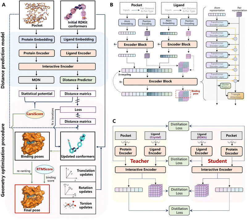 |
| | Fig. 1 Schematic view of (A) the overview of CarsiDock, (B) the architecture of the DL-based distance prediction model in CarsiDock, and (C) the self-distillation pipeline adopted in CarsiDock. | |
The distance prediction model (Fig. 1B) can be divided into five major components, including two independent embedding blocks, two independent encoder blocks, an interactive encoder block, a distance prediction block and a mixture density network (MDN) block. Specifically, the initial atomic tokens and distance matrices of the protein and ligand are first fed into the embedding layers to obtain their initial atom and pair representations, followed by an independent encoder block for both the ligand and protein to update the corresponding representations. Then the learned representations are input into the interactive encoder block to extract the cross-pair representation of the ligand and protein, and the outputs are either fed into the distance prediction block to obtain the distance matrices or processed by the MDN block to learn the parameter vectors to determine a mixture density model, from which a statistical potential could be obtained to aid the subsequent selection of the final binding pose. The model is pre-trained on millions of docking complexes produced by Glide SP and then fine-tuned on crystalized structures using a tailored self-distillation pipeline (Fig. 1C) along with two data augmentation strategies (i.e., the introduction of decoy compounds to replace the portion of the original crystalized ligands and the utilization of pockets with adjustable sizes).
Considering that directly reconstructing the distance matrices into coordinates may easily result in significant distortions in a molecule, here we optimize the coordinates of the ligand pose by adjusting the translations, rotations and torsion angles of the initial ligand conformers, whose objective is to force the updated distances to get closer to the ones output from the model. Fed with different initial RDKit conformers for a specific ligand, multiple binding poses could be generated by repeating this operation, and then they are ranked by CarsiScore that is defined as the weighted sum of the distance losses and the statistical potential, thus resulting in the final binding pose. The binding strength of the final binding pose is estimated by RTMScore,39 a MLSF developed in our previous study that exhibits extremely outstanding screening power.
CarsiDock achieves state-of-the-art performance for reproducing near-native binding poses
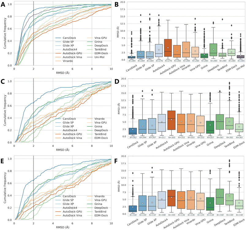
The docking accuracy of CarsiDock is first estimated on the widely-recognized PDBbind-v2016 core set (the main component of the CASF-2016 benchmark),40 and compared with that of 7 popular conventional docking programs (i.e., Glide SP,10 Glide XP,11 AutoDock4,6 Vina,8 Vinardo,41 AutoDock-GPU15 and Vina-GPU16) and 5 recently developed DL-guided approaches (i.e., Gnina,23 DeepDock,24 TankBind,30 EDM-Dock35 and Uni-Mol36). It should be noted that all the baselines here are not retrained for specific datasets, and instead they are executed directly through executable scripts and the saved models provided by the official repositories, so the performance of some methods (e.g., TankBind) may be overestimated to some extent due to the potential overlaps between the training and test sets. Despite this, the results presented in Table 1 and Fig. 2 still demonstrate the overwhelming superiority of our approach. Specifically, CarsiDock could successfully reproduce 89.82% of the top-ranked poses within RMSD ≤ 2.0 Å of the native binding poses, with the average RMSD across all the samples as low as 1.165 Å, while the second-ranked Uni-Mol could just obtain a corresponding top1 success rate of 81.75% and average RMSD of 1.436 Å, suggesting that the introduction of multiple strategies in our approach could be indeed beneficial to the improvement of the docking accuracy. The superior performance could be further verified through the cumulative distribution plots (Fig. 2A), where our approach could consistently outperform the baselines under multiple different RMSD thresholds (except for the overrated TankBind when the RMSD threshold is above 3.0 Å).
Table 1 Docking accuracy in terms of the top1 success rate (RMSD ≤ 2.0 Å) and average RMSD value on the PDBbind core set and time-split set
| Methods |
Core set (285) |
Time split (363) |
Time split (141)a |
| Top1 success rates (%) |
Average RMSDb (Å) |
Top1 success rates (%) |
Average RMSD (Å) |
Top1 success rates (%) |
Average RMSD (Å) |
|
This set removes the samples that have duplicated receptors as the fine-tuning set.
The complexes failing in docking are directly omitted to calculate the average RMSD.
The pose with the lowest RMSD value across the 10 runs is simply employed as the final pose.
|
| Glide SP |
64.91 |
2.206 |
43.53 |
3.551 |
37.59 |
3.642 |
| Glide XP |
65.61 |
2.218 |
44.35 |
3.754 |
39.01 |
3.931 |
| AutoDock4 |
46.74 |
3.449 |
23.14 |
5.055 |
16.31 |
5.132 |
| AutoDock Vina |
52.28 |
3.091 |
32.23 |
5.153 |
24.82 |
5.656 |
| Vinardo |
48.07 |
3.643 |
30.58 |
5.297 |
29.08 |
5.614 |
| AutoDock-GPU |
39.86 |
4.189 |
19.01 |
5.821 |
15.60 |
5.752 |
| Vina-GPU |
51.23 |
2.989 |
33.33 |
4.741 |
28.37 |
5.293 |
| Gnina |
72.63 |
1.875 |
49.02 |
3.957 |
44.93 |
3.751 |
| DeepDock |
44.91 |
3.550 |
19.01 |
5.523 |
14.18 |
6.205 |
| TankBind |
68.42 |
1.860 |
18.46 |
5.102 |
4.26 |
6.148 |
| EDM-Dockc |
46.32 |
2.631 |
41.05 |
3.353 |
36.88 |
3.825 |
| Uni-Mol |
81.75 |
1.436 |
— |
— |
— |
— |
|
CarsiDock
|
89.82
|
1.165
|
66.30
|
2.354
|
63.57
|
2.346
|
 |
| | Fig. 2 Prediction accuracy of docking programs based on (A and B) the PDBbind-v2016 core set, (C and D) time split of the PDBbind-v2020 dataset, and (E and F) a smaller time-split set in terms of (A, C and E) cumulative distributions of the RMSD values and (B, D and F) average RMSD values. The dotted lines in the cumulative distribution plots indicate a 2.0 Å RMSD cutoff, while the white square in the box plot denotes the mean value of each statistic. | |
Given that the core set is a high-quality subset of the whole PDBbind dataset and the complexes in it may be easier to be predicted than the average (Fig. S1†), we follow Stärk et al.29 to retrain CarsiDock according to the time split of the PDBbind-v2020 dataset, i.e., using a subset of 363 (or 141) complexes released in 2019 or later as the test set and the older ones as the training and validation sets. Here we majorly compare our approach with the traditional docking programs since those DL models (except TankBind) have involved those complexes for training. As expected, the indicators of all the approaches tested here decrease a lot, indicating a more difficult scenario that has been mimicked. However, our approach could still achieve a top1 success rate of 66.30% and an average RMSD of 2.354 Å, and retain a comparable performance on the smaller set with the corresponding indicators as high as 63.57% and 2.346 Å. In contrast, the best-performing traditional approach Glide XP could just obtain the corresponding metrics of 44.35%, 3.754 Å, 39.01% and 3.931 Å; Gnina that employs a 3D convolutional neural network-based scoring function for rescoring performs a little better (49.02%, 3.957 Å, 44.93% and 3.751 Å), but is still far worse than our approach. We also plot the cumulative distribution of the top1 success rates across different RMSD thresholds (Fig. 2C and E), and still, CarsiDock always performs better than the baselines, which further demonstrates the robustness of our approach.
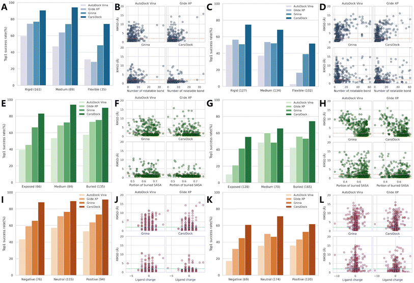
We further explore the impacts of three potentially key contributing factors, i.e., the number of rotatable bonds of ligands (Nrot), the portion of the ligand buried solvent accessibility surface area (pbSASA), and the ligand net charge, on the docking accuracy of CarsiDock, with three representative methods, i.e., AutoDock Vina, Glide XP and Gnina as the controls. As shown in Fig. 4A–D, Nrot that directly determines the searching freedoms inevitably exerts a significant influence, whether on AutoDock Vina guided by a heuristic search algorithm (top1 success rates decrease from 59.63% to 31.43% on the core set and from 50.40% to 2.94% on the time-split set with an increase in Nrot) or Glide XP that employs an exhaustive search (74.53% vs. 28.57% on the core set; 56.69% vs. 16.67% on the time-split set). The introduction of a MLSF for rescoring can to some extent improve the performance on more flexible ligands (e.g., Gnina vs. Vina: 48.57% vs. 31.43% on the core set and 39.22% vs. 2.95% on the time-split set), but there is no doubt that our approach can enhance the docking accuracy on the flexible cases to a new level, with the corresponding success rates for two sets up to 74.29% and 51.96%, respectively. pbSASA is also an important factor, and larger exposure to the solvents generally suggests worse performance (Fig. 4E–H). The empirical scoring functions embedded in AutoDock and Glide XP cannot effectively recognize the interactions with the solvents, thus resulting in their extremely poor performance for exposed cases (39.39% vs. 57.78% and 10.16% vs. 42.42%; 45.45% vs. 73.33% and 21.09% vs. 55.76%); however, DL-guided approaches (i.e., Gnina and CarsiDock) can capture these interactions from the training data, facilitating their weaker sensibility to pbSASA. The impact of the ligand net charge is not so distinct, but it can still be inferred from Fig. 4I–l that the poses for the negatively charged ligands are a little harder to be predicted, and our CarsiDock can consistently produce more stable results than the other approaches.
CarsiDock demonstrates excellent generalization capability on an external re-docking dataset
Time-split sets cannot completely avoid the impacts of the proteins that have already been seen in the pretraining stage, so we further test our approach on the PoseBusters benchmark set developed very recently,42 where a total of 428 crystal complexes released from 2021 onwards are collected. Considering that both the pretraining and finetuning stages of our approach just involve the proteins in the PDBbind-v2020 general set, where all the proteins were released before 2020, the training and testing sets shall not have any intersection at the level of PDB entry.
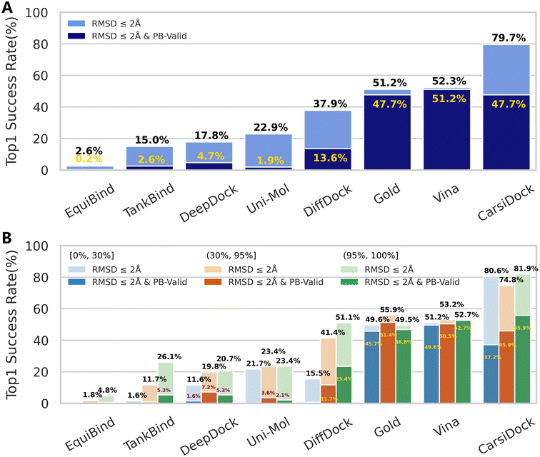
As shown in Fig. 3A, CarsiDock could achieve a top 1 success rate of 79.7%, significantly higher than that of all the baseline approaches reported before; when considering the various checks related to physical validity (PB-validity), the indicator decreases to 47.7%, slightly worse than that of the classical method AutoDock Vina (51.2%), but still superior to that of the other DL-based approaches. Further analysis (Fig. S2†) indicates that the potential clashes between the predicted poses and the protein may majorly account for the remarkably decreased performance with the consideration of PB-validity. As for this, we prefer to regard our approach as a strategy of soft-docking to treat protein flexibility, where the interatomic van der Waals interactions are softened and small levels of overlaps between the receptor and ligand shall be allowed.43,44
 |
| | Fig. 3 Prediction accuracy of docking programs based on the PoseBusters benchmark set (428 cases) indicated by (A) the overall top1 success rate and (B) top1 success rates across different thresholds (i.e., (0%, 30%], (30%, 95%] and (95%, 100%]) stratified by using sequence identity relative to the PDBbind-v2020 general set. | |
 |
| | Fig. 4 The impact of (A–D) the number of rotatable bonds of the ligand (rigid: ≤5 bonds; medium: 5–9; flexible: ≥10), (E–H) the portion of ligand buried solvent accessibility surface area (exposed: ≤0.6; medium: 0.6–0.65; flexible: ≥0.65), and (I–L) the ligand net charge on (A, C, E, G, I and K) the top1 success rates with a RMSD threshold of 2.0 Å and (B, D, F, H, J and L) RMSD values based on (A, B, E, F, I and J) the PDBbind-v2016 core set and (C, D, G, H, K and L) time-split set of the PDBbind-v2020 dataset. The dotted lines in the scatter plots indicate a 2.0 Å RMSD cutoff. | |
We also follow Buttenschoen et al.42 to stratify the proteins in the PoseBusters set by using sequence identity relative to the PDBbind-v2020 general set. It is shown in Fig. 3B that CarsiDock can obtain balanced performance across different thresholds (i.e., (0%, 30%], (30%, 95%] and (95%, 100%]), and the metric remains high (80.6%) even when the sequence identity to the training set is below 30%, suggesting its excellent generalization.
CarsiDock can maintain the topological reliability of the binding poses
One of the major obstacles of previous DL-guided docking models that impedes their further applications in real-world scenarios is the distortion of the topological structures of the generated poses. Although the introduction of some post-processing strategies such as aligning the pose to the RDKit-yielded conformers (EquiBind29) or minimizing the binding pose with an energy-based force field (EDM-Dock35) could to some extent correct the bonds and angles, they always lead to a decreased docking accuracy and even a significantly increased time consumption if conducting energy minimization. To this end, we introduce an improved local searching strategy, where the distance matrices are reconstructed into the final binding pose by tuning not only the translations and rotations but the torsion angles of the initial ligand conformers, with the guidance of a scoring function learned beforehand.
The aforementioned PoseBusters benchmark has involved the checking of topological reliability, and here we define two additional metrics to aid the evaluation, one is the difference in the bond lengths/angles between the predicted and the crystalized poses as a percentage of the latter, where the bond length/angle for a pose is determined either using the mean (PCTmean) or the maximum (PCTmax) one within the whole molecule, and the other is the root mean square deviation of the bond lengths/angles (RMSDBL/RMSDBA) derived from the RMSD. As shown in Fig. 5A–C, compared with traditional Glide XP and DL-based Uni-Mol and TankBind, the bond lengths and bond angles given by our approaches are closer to those of the crystalized binding poses. We further examine the detailed structures of three representative ligands (PDB entries: 1EBY, 1H22 and 1BCU) and present them in Fig. 5D. As can be seen, the poses predicted by CarsiDock exhibit almost the same topological structures as the native poses; Glide XP performs a little worse in terms of the indicators mentioned above, but can also generate visibly reasonable bonds and angles. As for the poses yielded by Uni-Mol, we can observe several significantly stretched bonds and angles, as well as the destroyed coplanarity of the benzene rings in most cases. The poses produced by TankBind are far more terrible, most of which huddle into a ball and are even hard to be recognized. Hence, though Uni-Mol and TankBind could substantially outperform the conventional approaches in terms of docking accuracy, the poor quality of the generated poses has proved their unreliability; in contrast, our approach could maintain the high-quality topological structures of the binding poses, which shall be considered as a premise of its better applicability.
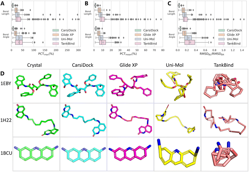 |
| | Fig. 5 Topological reliability of docking programs evaluated by (A) PCTmean, (B) PCTmax and (C) RMSDBL/RMSDBA, as well as (D) three representative ligand conformations (PDB entries: 1EBY, 1H22 and 1BCU) yielded by different docking programs. The white square in the box plot denotes the mean value of each statistic. | |
CarsiDock stays competitive in the scenario of cross docking or even when the protein is apo
Considering that the above experiments only involve the re-docking of crystalized ligands into their original protein entries, which may ignore the potential impacts of protein flexibility in real-world scenarios, we also turn to two forks of the PDBbind-v2016 core set, i.e., the PDBbind-CrossDocked-Core45 and APObind-Core46 sets, to investigate how CarsiDock could perform in the more complex scenarios of cross docking or even when the protein is apo. Here some DL-guided approaches including DeepDock, EDM-Dock, TankBind, and Uni-Mol are abandoned either due to the poor topological reliability of their produced poses or the extremely high computational consumption.
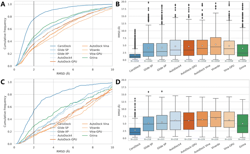
As presented in Table 2 and Fig. 6, the prediction accuracy of all these approaches decreases a lot in comparison to the corresponding re-docking results, but our method stays competitive. Specifically, CarsiDock could obtain a top1 success rate of 75.09% and an average RMSD of 1.734 Å on the cross-docking dataset, and the corresponding indicators are maintained at 50.66% and 2.778 Å when employing the apo proteins for docking, while the second-ranked Gnina could just obtain corresponding metrics of 44.71%, 3.980 Å, 27.07% and 5.013 Å. Though CarsiDock cannot explicitly treat the residues as flexible, the powerful fitting capability of the DL algorithm enables it to ignore the fluctuations of certain residues, thus leading to its competitive docking accuracy here.
Table 2 Docking accuracy in terms of the top1 success rate (RMSD ≤ 2.0 Å) and average RMSD value on the PDBbind-CrossDocked-Core set and APObind-Core set
| Methods |
PDBbind-CrossDocked-Core (1058) |
APObind-Core (229) |
| Top1 success rates (%) |
Average RMSDa (Å) |
Top1 success rates (%) |
Average RMSD (Å) |
|
The complexes failing in docking are directly omitted to calculate the average RMSD.
|
| Glide SP |
40.64 |
4.119 |
16.59 |
5.197 |
| Glide XP |
39.41 |
4.243 |
13.97 |
5.529 |
| AutoDock4 |
32.79 |
4.667 |
17.43 |
6.088 |
| AutoDock Vina |
27.88 |
4.891 |
13.10 |
6.448 |
| Vinardo |
27.32 |
5.325 |
11.35 |
6.662 |
| AutoDock-GPU |
33.75 |
4.616 |
18.35 |
5.989 |
| Vina-GPU |
27.60 |
4.834 |
11.79 |
6.270 |
| Gnina |
44.71 |
3.980 |
27.07 |
5.013 |
|
CarsiDock
|
75.09
|
1.734
|
50.66
|
2.778
|
 |
| | Fig. 6 Prediction accuracy of docking programs based on (A and B) the PDBbind-CrossDocked-Core set and (C and D) APObind-Core set in terms of (A and C) the cumulative distributions of the RMSD values and (B and D) average RMSD values. The dotted lines in the cumulative distribution plots indicate a 2.0 Å RMSD cutoff, while the white square in the box plot denotes the mean value of each statistic. | |
CarsiScore can well fulfill its duty of internal binding pose ranking
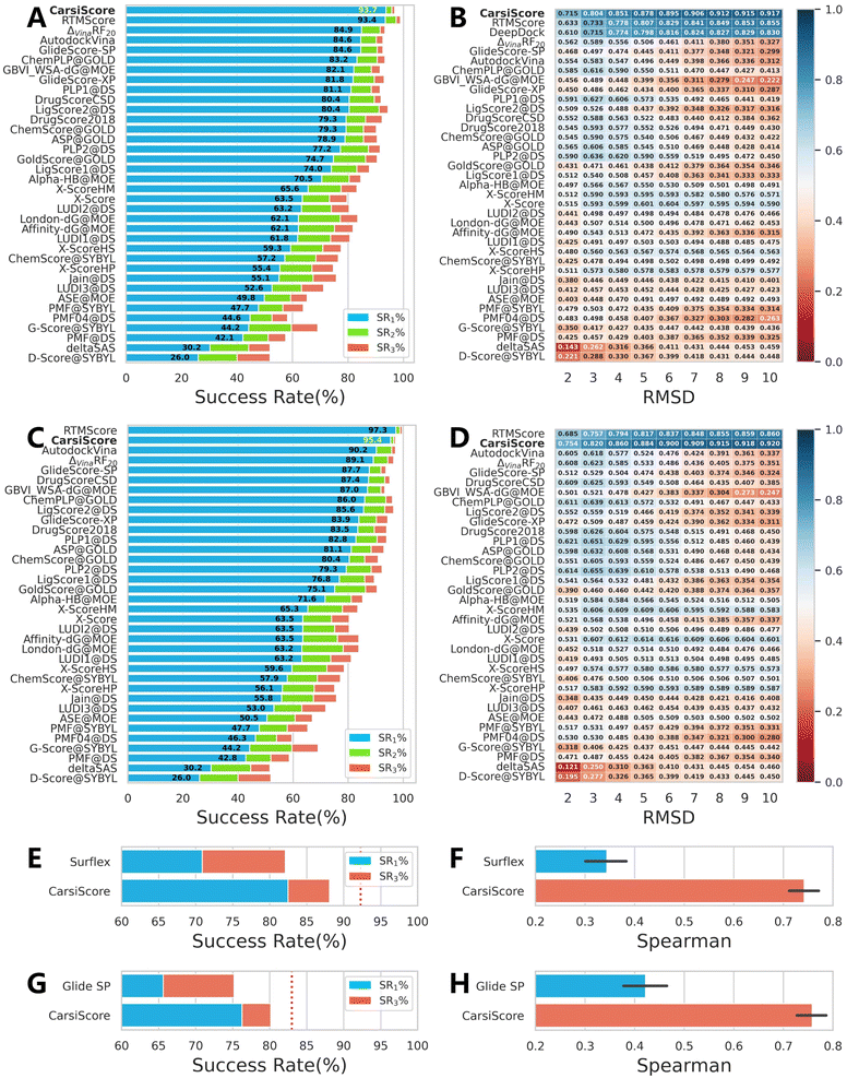
As a critical component of CarsiDock, CarsiScore that is first proposed here is specifically assessed as an independent SF on the standard CASF-2016 benchmark, and compared with 33 traditional SFs reported by Su et al.40 (Fig. 7) and some representative MLSFs (Table 3) in terms of the capability to distinguish near-native binding poses from incorrect poses (docking power). Overall, CarsiScore could successfully identify the top-ranked pose within RMSD ≤ 2.0 Å of the native binding pose in 93.7%/95.4% of cases without/with the crystalized poses in the test set, which is comparable to the performance of our previously developed RTMScore,39 a MLSF that relies on a similar statistical potential for scoring (the corresponding indicators are 93.4% and 97.3%), but significantly better than the other compared approaches. The results of binding funnel analysis (Fig. 7B and D) further indicate the superiority of CarsiScore for precise pose ranking, where it exhibits even higher Spearman correlation coefficients than RTMScore across almost all the RMSD windows.
 |
| | Fig. 7 Docking powers of CarsiScore on the CASF-2016 benchmark indicated by (A and C) the success rates at the top 1%, 2% and 5% levels and (B and D) the binding funnel analysis either (A and B) without or (C and D) with the crystalized poses in the test set, and on the poses generated by (E and F) Surflex-Dock and (G and H) Glide SP indicated by (E and G) the success rates at the top 1% and 3% levels and (F and H) the average Spearman correlation coefficient across different complexes. For the binding funnel analysis, the x-axis denotes the RMSD range (e.g., [0–2 Å] [0–3 Å], etc.), where the Spearman correlation coefficients between the RMSD values and the predicted scores are calculated. | |
Table 3 Docking power of multiple scoring functions in terms of the top 1 success rate (RMSD ≤ 2.0 Å) on the CASF-2016 benchmark
| Scoring function |
Excluding native poses in the test set |
Including native poses in the test set |
| Autodock Vina7,40 |
0.846 |
0.902 |
| ChemPLP@GOLD9,40 |
0.832 |
0.860 |
| GlideScore-SP10,40 |
0.846 |
0.877 |
| KORP-PL70 |
0.856 |
0.891 |
| ΔVinaRF20 (ref. 71) |
0.849 |
0.891 |
| ΔVinaXGB72 |
— |
0.916 |
| ΔLin_F9XGB73 |
— |
0.867 |
| OnionNet-SFCT + Vina74 |
— |
0.937 |
| DeepRMSD + Vina75 |
0.916 |
0.944 |
| DeepBSP76 |
0.872 ± 0.014 |
0.885 ± 0.013 |
| PIGNet77 |
0.870 |
— |
| DeepDock24 |
0.870 |
— |
| RTMScore39 |
0.934 ± 0.002 |
0.973 ± 0.012
|
|
CarsiScore
|
0.937
|
0.954 |
To ensure the comprehensiveness of the assessment, the indicators regarding the other three tasks in CASF-2016, i.e., scoring (the capability to produce binding scores in a linear correlation with experimental binding data), ranking (the capability to rank the known ligands of a specific target by using their binding scores) and screening (the capability to identify known binders from decoys), are also supplemented, as shown in Fig. S3.† Unfortunately, the performances of CarsiScore here are far worse than the average. It is not too surprising to see its poor scoring and ranking powers since the experimental binding affinity data are not involved in model training, and RTMScore that utilizes a similar strategy also performs not so well. As for the awful screening power, perhaps the involvement of large-scale docking complexes for model pre-training may partially account for it. Though these complexes could force the model to learn the docking modes given by existing docking programs, thus enhancing the performance for pose generation/ranking, after all, almost all of them are not real binding complexes, thereby increasing the difficulty to identify known binders from non-binders. However, as a built-in scoring scheme for pose ranking, the excellent docking power is enough for CarsiScore to exert its basic functions, and other tasks such as binding affinity prediction and virtual screening (VS) could be achieved by combining our CarsiDock with other customized rescoring approaches,47–49 just as we have done to embed RTMScore into existing docking programs.
We also test CarsiScore as a rescoring tool to re-rank the binding poses directly produced by Surflex-Dock50 or Glide SP, and explore whether the approach could be employed for pose selection for other docking methods. As shown in Fig. 7E–H, CarsiScore could indeed improve the pose quality for both the docking programs, with the top1 success rate increasing from 70.88% to 82.46% for Surflex-Dock and from 65.60% to 76.24% for Glide SP. When it comes to the average Spearman correlation coefficient of the binding poses across all the targets, the superiority of CarsiScore is more remarkable, with the corresponding indicators increasing from 0.344 to 0.741 for Surflex-Dock and from 0.422 to 0.758 for Glide SP, which further demonstrates the excellence of our approach in precise pose ranking.
CarsiDock can obtain excellent screening performance with RTMScore as the final scoring function
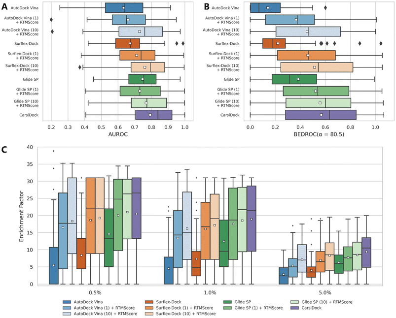
CarsiScore exhibits unsatisfactory screening power on the CASF-2016 benchmark, but we wonder how CarsiDock with RTMScore as the final scoring function will perform in large-scale VS campaigns. Therefore, we further conduct several retrospective screening experiments on the DEKOIS2.0 (ref. 51) dataset, and present the results measured by AUROC, BEDROC and EFs in Table 4 and Fig. 8, with the data from our previous study39 as a comparison. As can be observed, CarsiDock could obtain a mean AUROC of 0.793, BEDROC of 0.568, EF0.5% of 20.46, EF1% of 18.91 and EF5% of 9.38, significantly superior to those of the widely employed docking programs Glide SP, Surflex-Dock and AutoDock Vina (the corresponding indicators of the best-performing Glide SP are 0.747, 0.385, 14.61, 12.47 and 6.30). The involvement of RTMScore for rescoring could improve the early recognition performance for these traditional docking approaches; moreover, owing to the high sensitivity of RTMScore to the quality of the binding poses, the cases of generating at most 10 poses for rescoring generally performs better than those just based on the top-ranked poses. Interestingly, CarsiDock that only relies on the top-ranked poses for the RTMScore rescoring can achieve comparable performance to the case using at most 10 poses produced by Glide SP (mean BEDROC: 0.568 vs. 0.558; EF0.5%:20.46 vs. 20.99; EF1%: 18.91 vs. 18.53; EF5%: 9.38 vs. 8.45), let alone the case just employing the optimal poses predicted by Glide SP (mean BEDROC = 0.522; EF0.5% = 20.08; EF1% = 17.53; EF5% = 7.76) or those based on the poses generated by Surflex-Dock and AutoDock Vina. These findings indicate that CarsiDock embedded with RTMScore can be indeed applicable to docking-based VS; on the other hand, these results also suggest the superior docking accuracy of our approach, which could be generalized to more complex VS scenarios to provide more reliable binding poses for high-precision rescoring.
Table 4 Screening performance of multiple approaches on the DEKOIS2.0 dataset
| Docking methods |
Rescoring methods |
Number of poses for rescoring |
AUROC |
BEDROC (α = 80.5) |
EF0.5% |
EF1% |
EF5% |
| Mean |
Med |
Mean |
Med |
Mean |
Med |
Mean |
Med |
Mean |
Med |
|
The results based on Glide SP, Surflex-Dock and AutoDock Vina are directly retrieved from our previous study.39
CarsiDock here employs RTMScore as the final scoring function to estimate the binding strength of the protein–ligand complexes.
|
| Glide SPa |
— |
— |
0.747 |
0.754 |
0.385 |
0.314 |
14.61 |
13.30 |
12.47 |
9.61 |
6.30 |
5.97 |
| RTMScore |
Top-ranked |
0.730 |
0.731 |
0.522 |
0.540 |
20.08 |
24.79 |
17.53 |
18.66 |
7.76 |
7.62 |
| RTMScore |
At most 10 |
0.768 |
0.773 |
0.558 |
0.602 |
20.99
|
26.31 |
18.53 |
21.73
|
8.45 |
8.64 |
| Surflex-Dock |
— |
— |
0.673 |
0.675 |
0.220 |
0.180 |
8.36 |
4.43 |
7.30 |
4.77 |
4.00 |
3.50 |
| RTMScore |
Top-ranked |
0.711 |
0.738 |
0.461 |
0.464 |
18.59 |
22.14 |
16.04 |
16.69 |
6.93 |
6.50 |
| RTMScore |
At most 10 |
0.760 |
0.793 |
0.514 |
0.544 |
19.24 |
22.14 |
17.13 |
19.08 |
8.33 |
8.50 |
| AutoDock Vina |
— |
— |
0.633 |
0.637 |
0.140 |
0.070 |
5.46 |
0.00 |
4.51 |
0.00 |
2.82 |
2.38 |
| RTMScore |
Top-ranked |
0.659 |
0.651 |
0.367 |
0.376 |
16.54 |
17.71 |
13.39 |
14.28 |
5.29 |
5.00 |
| RTMScore |
At most 10 |
0.729 |
0.760 |
0.455 |
0.463 |
18.36 |
17.71 |
16.18 |
15.08 |
7.09 |
7.00 |
|
CarsiDock
|
0.793
|
0.839
|
0.568
|
0.632
|
20.46 |
26.55
|
18.91
|
21.43 |
9.38
|
10.48
|
 |
| | Fig. 8 Screening performance of multiple approaches on the DEKOIS2.0 data set, in terms of (A) AUROC, (B) BEDROC (α = 80.5) and (C) enrichment factors at different thresholds (0.5%, 1.0%, and 5.0%). The white square in the box plot denotes the mean value of each statistic. CarsiDock here employs RTMScore as the final scoring function to estimate the binding strength of the protein–ligand complexes. | |
CarsiDock can recover the key interactions in crystalized structures
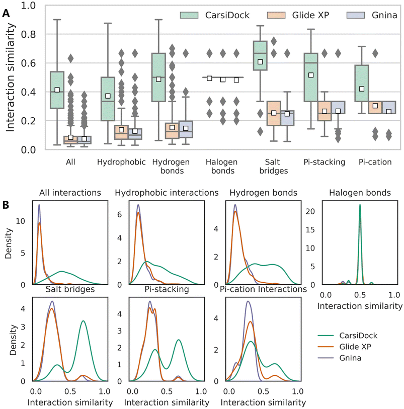
The reliability of CarsiDock is also assessed from the perspective of learning crucial interactions, with Glide XP and Gnina that could not only obtain acceptable docking accuracy but maintain the reliable topological structures as the controls. Specifically, six types of noncovalent interactions, i.e., hydrophobic interactions, hydrogen bonds, halogen bonds, salt bridges, and pi–stacking and pi–cation interactions, defined by protein–ligand interaction profiler (PLIP),52 are detected to calculate the interaction similarities between the predicted and the crystalized poses. When the similarity is defined at the residue level (Fig. S4†), CarsiDock could obtain generally higher interaction similarities than Glide XP and Gnina for almost all types of interactions (except the halogen bonds and the pi–cation interactions, potentially due to the lack of samples) in terms of both the average similarity (Fig. S4A†) and distributions (Fig. S4B†); when using the more difficult atom-level similarity as indicators (Fig. 9), the superiority of our approach seems more dominant, suggesting its greater experience in the precise capturing of atomic interactions.
 |
| | Fig. 9 (A) Interaction similarity at the atom level and (B) the corresponding distributions for seven types of interactions of the poses predicted by three docking programs, including all interactions, hydrophobic interactions, hydrogen bonds, halogen bonds, salt bridges, and pi–stacking, and pi–cation interactions. The white square in the box plot represents the mean value of each statistics. | |
Two cases (PDB entries: 2XII and 4HGE) are further presented to demonstrate the detailed differences in the poses produced by these docking programs and the crystalized poses. For 2XII (Fig. 10A–D), though the poses predicted by different docking methods could yield similar RMSD values with respect to the crystal pose (0.309 Å, 0.486 Å and 0.564 Å for CarsiDock, Glide XP and Gnina, respectively), the slight fluctuation of the 9-fluorenone region in the poses generated by Glide XP and Gnina leads to the loss of crucial pi–cation interactions with Arg262 as well as multiple hydrophobic interactions with Arg262 and Glu288. Regarding 4HGE (Fig. 10E–H), the pose predicted by CarsiDock even has worse RMSD values (0.718 Å vs. 0.206 Å and 0.322 Å) due to the slight shift of the overall structure, but it could still obtain the highest similarity score. The minor translational difference does not make it lose too many key interactions; in contrast, the poses from Glide XP and Gnina lose the crucial hydrogen bond with Ser936, and Gnina even forces the pose to form an excessive halogen bond with Gly861, thus leading to their worse reconstruction of interactions here.
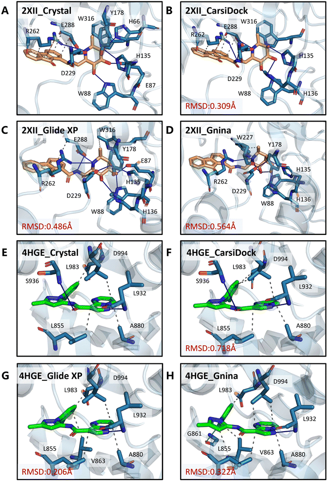 |
| | Fig. 10 Binding modes of (A and E) the crystalized poses and poses produced by (B and F) CarsiDock, (C and G) Glide XP and (D and H) Gnina for the PDB entries 2XII and 4HGE. The proteins and ligands are colored in blue and orange/green, respectively. Grey dashed lines denote the hydrophobic interactions, blue solid lines denote the hydrogen bonds, orange dashed lines denote the pi–cation interaction, and the green-cyan solid line denotes the halogen bond. | |
Ablation study
The superior docking accuracy of our approach can be attributed to the incorporation of multiple innovative designs, i.e., pre-training the model on a large-scale docking dataset, introducing the triangle self-attention mechanism and MDN in the model architecture, and the self-distillation pipeline for model training, as well as applying multiple initial ligand conformers for data augmentation. On the other hand, the involvement of two data augmentation strategies at both the ligand and pocket levels in model training shall be the major driving force to enhance model generalization, thus improving the screening performance. Here we first conduct the ablation experiments on the PDBbind-v2016 core set to explore whether the former five main strategies could indeed be beneficial to the enhancement of docking accuracy (Table 5), and then emphatically discuss the impacts of the two data augmentation strategies on the docking accuracy on multiple docking datasets and the screening performance on the DEKOIS2.0 dataset, with the results summarized in Table 6 and Table S1.†
Table 5 Impacts of several strategies on the docking accuracy based on the PDBbind-v2016 core set
| Strategya |
Amount of data for pre-training |
Top1 success rates (%) |
Average RMSD (Å) |
|
All these models are trained without decoy compound and pocket augmentations.
|
| Without pre-training |
— |
82.81 |
1.491 |
| Pre-training using only a small amount of data |
∼1.5 M |
89.12 |
1.137 |
| Without triangular self-attention and pre-training |
— |
78.25 |
1.760 |
| Without self-distillation |
∼8 M |
89.47 |
1.019 |
| Without MDN |
∼8 M |
90.53 |
1.002 |
| Without conformer augmentation |
∼8 M |
91.58 |
1.021 |
| CarsiDock (without decoy compound and pocket augmentation) |
∼8 M |
92.28
|
0.982
|
Table 6 Impacts of two data augmentation strategies on the docking accuracy based on the PDBbind-v2016 core set and the screening performance based on the DEKOIS2.0 dataset
| Strategy |
PDBbind core set |
DEKOIS2.0 |
| Top1 success rates (%) |
Average RMSD (Å) |
AUROC |
BEDROC (α = 80.5) |
EF0.5% |
EF1% |
EF5% |
| Mean |
Med |
Mean |
Med |
Mean |
Med |
Mean |
Med |
Mean |
Med |
| Without decoy compound and pocket augmentation |
92.28
|
0.982
|
0.667 |
0.685 |
0.392 |
0.316 |
15.91 |
17.67 |
13.48 |
9.54 |
5.97 |
4.50 |
| Without decoy compound augmentation |
89.82 |
1.044 |
0.744 |
0.782 |
0.507 |
0.529 |
19.08 |
22.13 |
17.13 |
19.05 |
8.18 |
8.50 |
| CarsiDock |
89.82 |
1.165 |
0.793
|
0.839
|
0.568
|
0.632
|
20.46
|
26.55
|
18.91
|
21.43
|
9.38
|
10.48
|
Effect of pre-training.
One of the most primary innovations of our approach is the introduction of millions of docking complexes for pre-training, and hence the effect of pre-training is specifically investigated. As can be seen, the model directly trained on the PDBbind-v2020 dataset from scratch could just obtain a top1 success rate of 82.81% and an average RMSD of 1.491 Å; the corresponding indicators turn to 89.12% and 1.137 Å when using ∼1.5 M complexes for pre-training, and the values further increase to 92.28% and 0.982 Å with the involvement of ∼8 M complexes, indicating that pre-training indeed plays a critical role in performance improvement. Though the molecules randomly selected from the database shall be non-binders to the docked targets in almost all the cases, we can infer that these docking complexes shall contain a lot of physical information that is produced through the conventional docking process. The existence of these complexes could force the model to learn the meaningful protein–ligand interactions given by traditional docking programs (i.e., Glide SP), thus enhancing its performance for pose generation/ranking.
Effect of triangular self-attention.
Different from the conventional self-attention mechanism, triangular self-attention needs three nodes to update the representations, and thus is in better accordance with the geometric learning scenarios in 3D space. As expected, the ablation of triangular self-attention leads to the remarkable decrease of both the top1 success rate (78.25 vs. 82.81%) and the average RMSD (1.760 Å vs. 1.491 Å) on comparison to the model without pre-training, implying its importance to maintain the prediction accuracy.
Effect of MDN.
The introduction of MDN shall not only yield a statistical potential for the estimation of protein–ligand binding strengths but also force the model to learn the distance likelihood for each ligand–target pair, which could be considered as an inductive bias to aid the learning of distance matrices. Our inference could be verified by using Table 4, where the docking accuracy after the ablation of the MDN module will decrease from 92.28% to 90.53% in terms of the top1 success rate and from 0.982 Å to 1.002 Å regarding the average RMSD.
Effect of self-distillation.
Our approach could also benefit from the dedicatedly designed self-distillation pipeline, which facilitates the docking accuracy increasing from 89.47% to 92.28% and from 1.019 Å to 0.982 Å for the two indicators, respectively. The rich information stored in the teacher model can be well transferred to the Student model through the procedure, thus forcing the yielded binding poses to be closer to the crystalized ones.
Effect of ligand conformer augmentation.
Using ten initial ligand conformers rather than the one routine conformer in model training could be regarded as a data augmentation strategy. As expected, the model without conformer augmentation could just obtain a top1 success rate of 91.58% and average RMSD of 1.021 Å, which is slightly poorer than those given by the corresponding model initialized with multiple conformers. Considering that molecular docking shall be a dynamic process, the introduction of more initial coordinates could force the model to learn more docking paths for a specific ligand–target pair, thus enhancing the performance.
Impacts of decoy compound and pocket augmentations.
As shown in Table 6, the application of two data augmentation strategies in the fine-tuning stage will result in a minor decrease in docking accuracy on the PDBbind core set (e.g., average RMSD changes from 0.982 Å to 1.044 Å and 1.165 Å with the sequential introduction of pocket augmentation and decoy compound augmentation) and substantial decrease in prediction accuracy regarding the other three docking datasets (Table S1†), but significant improvement of screening performance (e.g., the corresponding mean EF1% increases from 13.48 to 17.13 and 18.91). We guess that a lot of noise yielded at either the ligand or the pocket level may majorly account for these phenomena, which on the one hand, may exert a negative effect on the learning of the binding modes for the known binding complexes, but on the other hand, enhance its decision-making capability when faced with more complex scenarios (e.g., the prediction of the binding modes for the non-binders). Additionally, these findings also suggest that DL-guided approaches with high docking accuracy do not necessarily indicate their good applicability in VS. It should be noted that all the ligands for these docking datasets are known binders, but it is very possible that non-binders will also obtain an ideal prediction. Hence, extra validation of a docking program from the perspective of screening is necessary, which is actually lacking for most previous DL-guided docking approaches.
Conclusion
In this work, we have reported a DL-guided docking method that exploits large-scale pre-training of millions of docking complexes for protein–ligand binding pose prediction. Our approach is composed of two primary stages, i.e., a DL model to predict protein–ligand distance matrices and a geometry optimization procedure to reconstruct the matrices into a credible binding pose. Besides the pre-training, multiple effective strategies such as the triangle self-attention mechanism to enhance geometric learning, the MDN to assist the learning of distance matrices and a self-distillation pipeline to aid model training are also incorporated, thus facilitating a noticeable performance improvement of our docking program in binding pose prediction in terms of both the prediction accuracy and the capability to reproduce crucial interactions in crystalized poses. The introduction of data augmentations in model fine-tuning could further improve the generalization of our approach, thereby leading to its excellent performance in docking-based VS when combined with high-precision rescoring. More importantly, the geometry optimization procedure executed by tuning the translations, rotations and torsion angles of the initial ligand conformers further enables our approach to maintain the topological reliability of the predicted binding poses, which shall be a premise of its better applicability. Finally, extensive ablation experiments are presented to demonstrate the effectiveness of multiple designs introduced in our approach. Although here we just focus on protein–ligand semiflexible docking, a scenario where the proteins are fixed as rigid, similar strategies could be also employed to explicitly take the protein flexibility into consideration, and further extended to the other more complex biosystems, such as protein-peptide, protein–protein and nucleic acid-ligand systems.
Methods
Dataset preparations
The PDBbind-v2020 general set that had been further preprocessed by Zhou et al.36 was employed as the core training set here. The preprocessing operations included adding missing atoms, manually fixing file-loading errors, and eliminating the structures highly similar to the ones in the CASF-2016 benchmark by taking both the protein sequence identity and ligand similarity into consideration, thus resulting in a total of 18![[thin space (1/6-em)]](https://www.rsc.org/images/entities/char_2009.gif) 404 complexes, which were randomly divided into the training and validation sets with a ratio of 9
404 complexes, which were randomly divided into the training and validation sets with a ratio of 9![[thin space (1/6-em)]](https://www.rsc.org/images/entities/char_2009.gif) :
:![[thin space (1/6-em)]](https://www.rsc.org/images/entities/char_2009.gif) 1.
1.
The complex dataset utilized for pre-training was created by docking 500 randomly selected compounds from the ChemDiv library into the pocket of each protein in the PDBbind-v2020 general set. The proteins and molecules were first prepared by using the Protein Preparation Wizard53 and LigPrep54 modules in Schrödinger 2020, respectively, with all the default settings, and then Glide SP was employed for docking. Only the pose with the highest docking score was retained for each protein–ligand pair, thus leaving a total of 9![[thin space (1/6-em)]](https://www.rsc.org/images/entities/char_2009.gif) 341
341![[thin space (1/6-em)]](https://www.rsc.org/images/entities/char_2009.gif) 657 docking complexes, in which 8
657 docking complexes, in which 8![[thin space (1/6-em)]](https://www.rsc.org/images/entities/char_2009.gif) 318
318![[thin space (1/6-em)]](https://www.rsc.org/images/entities/char_2009.gif) 054 complexes whose proteins were the same as those in the above-mentioned training set were employed for training and the other 1
054 complexes whose proteins were the same as those in the above-mentioned training set were employed for training and the other 1![[thin space (1/6-em)]](https://www.rsc.org/images/entities/char_2009.gif) 023
023![[thin space (1/6-em)]](https://www.rsc.org/images/entities/char_2009.gif) 603 for validation.
603 for validation.
For each protein–ligand pair, the protein was truncated to the binding pocket defined as the residues within 5.0–7.0 Å around the co-crystalized ligand to save the computational cost. Specifically, if one of the heavy atoms in a residue was within the predefined threshold, this residue was considered as a component of the pocket. As for each ligand, its initial coordinates were determined using the experimental-torsion basic knowledge distance geometry (ETKDG)55 algorithm in RDKit,56 and a total of 10 conformers were generated for each ligand. The initial inputs for each pocket/ligand included a group of atomic type tokens to record the atomic type for each atom, the intramolecular atomic distance matrix, and the initial coordinates for each atom. To map the atomic type tokens into a series of consecutive integers, we predefined a dictionary that contained 26 common atomic types (C, N, O, S, H, Cl, F, Br, I, Si, P, B, Na, K, Al, Ca, Sn, As, Hg, Fe, Zn, Cr, Se, Gd, Au, and Li) for ligands and 5 atomic types (C, N, O, S, and H) for proteins. Besides, we added four auxiliary tokens in the dictionary, i.e., [CLS] for recording the beginning of the sequence, [SEP] for recording the ending of the sequence, [UNK] for recording the unknown atomic type, and [PAD] for padding sequences to a fixed length.
Framework of CarsiDock
Fig. 1 depicts an overview of CarsiDock, which consists of a DL model to predict the protein–ligand atomic distance matrices and a geometry optimization procedure to reconstruct the distance matrices into a reliable binding pose. In this section we only introduce the framework of the DL model, and the geometry optimization details that are not involved in the training of CarsiDock will be provided in the later section.
The model architecture can be divided into five major components, including two independent embedding blocks, two independent encoder blocks, an interactive encoder block, a distance prediction block and a mixture density network (MDN)57 block. Specifically, the initial inputs for the ligand and protein are first fed into the embedding layers to obtain their initial atom and pair representations, followed by an independent encoder block for both the ligand and protein to update the atom and pair representations. Then the learned representations are input into the interactive encoder block to extract the cross-pair representation of the ligand and protein, and finally the outputs are either fed into the distance prediction block to obtain the distance matrices or processed by the MDN block to learn the parameter vectors to determine a mixture density model, from which a statistical potential could be obtained to guide the selection of the final binding poses.
Embedding blocks.
To obtain the initial atom representations, here we employ two independent embedding layers to map the atomic type tokens of the ligand and protein into their corresponding embeddings, thus resulting in a ligand embedding matrix  and a protein matrix
  , where Nl and Np are the numbers of the atoms for the ligand and protein, respectively, and d denotes the dimension of hidden representations.
We further adopt a spatial positional encoding strategy proposed by Zhou et al.,36 which relies on the atomic distance map and the resulting pair-type aware Gaussian kernel,58 for the description of the relative positions between different atoms in 3D space. The D-dimensional positional encoding of atom pair ij can be described as:
| |  | (1) |
where

is a Gaussian density function parametrized with
μ and
σ;
dij denotes the Euclidean distance between the atoms
i and
j, and
tij corresponds to the atomic types of pair
ij;

represents the affine transformation parametrized with
m and
n, which is employed to affine
dij to its corresponding atom types
tij;
μ,
σ,
u and
v are all learnable parameters. Then the initial representation for atom pair
ij (
q0ij) can be computed through the following equation:
where

and

are learnable parameters for linear projections, and GELU is a type of nonlinear activation. This operation guarantees the dimension of
q0ij the same as the number of the attention head
H employed in the following transformer encoder.
Independent encoder block.
In this module, we utilize an expanded transformer encoder59,60 framework to learn the intrinsic representations for both the ligand and protein. The updates of the atom representation for atom i (hil) and the pair representation for atom pair ij (qijl) in the lth layer are described as:| | | Qijk,l = WQk,lDropout(LN(hil)) | (3) |
| | | Kijk,l = WKk,lDropout(LN(hil)) | (4) |
| | | Vijk,l = WVk,lDropout(LN(hil)) | (5) |
| |  | (6) |
| | | hil+1 = ĥil+1 + Dropout(Øh2l(Dropout(GELU(Øh1l(LN(ĥil+1)))))) | (7) |
| |  | (8) |
where WQk,l, WKk,l,  ,
,  ,
,  and
and  are all learnable weights for linear layers; H and dk represent the number of attention head and the dimension of each head, respectively, and their product is the hidden dimension d; N represents the number of atoms for either the ligand or the protein; Dropout, LN, Concat and Softmax represent the dropout, layer normalization, concatenation and softmax operations, respectively, and GELU is a type of nonlinear activation.
We further introduce the triangular self-attention mechanism that is first proposed in the Evoformer28,61 module of AlphaFold2 to update the outputs from the last layer of the transformer encoder, thus not only enhancing model learning for 3D space but to some extent, reducing the computational cost. For the atom representation for atom i (hlasti) and the pair representation for atom pair ij (qlastij) from the last layer, a series of operations are exerted, including the “Outer product mean” operation to transform the atom representation into an update for the pair representation, the “Triangular multiplicative update” operation to update the pair representation by combining information within each triangle of atom pairs ij, ik and jk, the “Triangular self-attention” operation to further update the pair representation, and a transition layer to output the final pair representation zij. The algorithmic details are given in the ESI.†
| | | zij = Triangular_Attention(hlasti,qlastij) | (9) |
Interactive encoder block.
The learned representations for the ligand (hlig and zlig) and protein (hprot and zprot) are concatenated at both the atom and pair levels, thus resulting in the representations for the protein–ligand complex, i.e.,  and
and  , where Nl and Np are the numbers of the atoms in the ligand and protein, respectively. They are then fed into an encoder that has the same framework as the one in the previous module (a combination of a Transformer encoder and triangular attention) to learn the cross-pair representation from scratch with recycling.
Distance prediction block.
Here two projection layers are employed to project the outputs from the previous module into the distance matrices that are crucial for pose reconstruction. The protein–ligand pair distances can be obtained through:| | | DPLij = ELU(WPL2RELU(WPL1Concat([hligi,hprotj,zcrossij]))) + 1 | (10) |
where hligi and hprotj denote the updated representations for the ith atom of the ligand and the jth atom of the protein, respectively, and zcrossijdenotes the corresponding cross-pair representation;  and
and  are the weight matrices for linear projections; RELU and ELU are nonlinear activations. The distance matrix for the ligand is also updated as:
| | ![[D with combining circumflex]](https://www.rsc.org/images/entities/i_char_0044_0302.gif) Lij = WL2(LN(RELU(WL1(Concat([hligi, zligij])))) Lij = WL2(LN(RELU(WL1(Concat([hligi, zligij])))) | (11) |
| |  | (12) |
where hligi and zligij are the representations of atom i and pair ij in the ligand, respectively;  and
and  are weight matrices.
MDN block.
The representations from the interactive encoder block are simultaneously fed into an MDN to calculate three parameter vectors important for the construction of a mixture density model, including the means (μij), standard deviations (σij) and mixing coefficients (ρij):| | | μij = ELU(Wμ2(LN(RELU(Wμ1(Concat([hligi,hprotj,zcrossij])))))) + 1 | (13) |
| | | σij = ELU(Wσ2(LN(RELU(Wσ1(Concat([hligi,hprotj,zcrossij])))))) + 1.4 | (14) |
| | | ρij = Softmax(Wφ2(LN(RELU(Wφ1(Concat([hligi,hprotj,zcrossij])))))) | (15) |
where Wμ1, Wσ1, and  and Wμ2, Wσ2 and
  are weight matrices; Ng is the number of Gaussians to compose the mixture density model. The model can well simulate the probability density distribution of the distance between protein–ligand atom pairs, thus serving as a guidance for the subsequent selection of the final binding pose.
Model training
We pre-train the model on millions of docking complexes yielded by Glide SP and then fine-tune the model on crystalized structures. The pre-training and fine-tuning stages share the same model architecture except for some specific hyperparameters. The detailed hyperparameter settings can be found in Table S2.†
Self-distillation.
To further improve the model performance, a dedicatedly designed self-distillation pipeline is introduced into the fine-tuning stage. Specifically, two networks (denoted as Student and Teacher) that share the same architecture but different inputs are constructed. The Student model relies on RDKit to yield the initial coordinates for the ligand while the corresponding coordinates for the Teacher model are directly inherited from the crystal pose. Considering that crystal poses shall be much closer to the true poses than those produced by RDKit, the hidden representations learned from the Teacher shall be more informative and less noisy, and therefore a distillation loss could be designed to capture these information gaps. As shown in Fig. 1C, for the outputs from all the encoders, we can introduce an individual distillation loss, whose objective is to force the representations from the Student to approach those from the Teacher. Of note, the information gap for the outputs from the protein encoder shall come from different dropouts in two sub-models, and the existence of the loss can still force the two outputs to be consistent with each other, thereby enhancing the model stability in inferencing.63 To update the model, we stop the gradient calculation on the Teacher and force the network to propagate gradients only through the Student, and then the loss can be computed as:| |  | (20) |
where ht and hs denote the output representations for Teacher and Student, respectively, Hdis denotes the number of representations that is set to 6 here (3 encoders with both the atom and pair representations), and MSE denotes the mean square error operation. Hence, the final loss function employed in the fine-tuning stage can be described as:| |  | (21) |
where  and
and  can be further described as the weighed sum of
  ,
,  and
and  , as:
, as:| |  | (22) |
where wdistillation, wcross_dist, wlig_dist and wMDN are adjustable weights. Of note, considering that the self-distillation pipeline is just introduced in the fine-tuning stage, the loss function used in the pre-training stage is simply calculated through eqn (22).
Data augmentations at both the ligand and pocket levels.
We also employ two data augmentation strategies in the fine-tuning stage to enhance the generalization capability of our approach, i.e., the introduction of decoy compounds to replace the portion of the original crystalized ligands, and the utilization of pockets with adjustable sizes. For a specific ligand–pocket pair in each epoch, each crystalized ligand has a chance of 20% to be replaced by the corresponding decoy ligand (randomly selected from 500 docked compounds for pre-training); meanwhile, instead of the pocket defined as the residues within the fixed 6.0 Å around the co-crystalized ligand, a pocket randomly selected from the pre-generated 10 pockets with cutoffs of 5.0–7.0 Å is employed. For the preparation of pockets, two pockets defined with cutoffs of 5.0 Å and 7.0 Å are first produced, and then the differences of their residues are randomly added to a pocket of 5.0 Å, thus resulting in 10 augmented pockets.
Geometry optimization
This procedure intends to convert the outputs from the DL model into the final binding pose with the hierarchical guidance of three customized scoring schemes (i.e., distance loss, CarsiScore, and RTMScore). Specifically, fed with 10 initial RDKit conformers for each ligand, the neural networks could output 10 groups of distance matrices and 10 mixture density models. To obtain more diverse poses, the 10 initial poses are combined with 10 groups of distance matrices in a pairwise manner (rather than a consistent one-to-one match) to conduct coordinate transformations, thus resulting in a total of 100 potential binding poses. Then, these poses are ranked by CarsiScore, which consists of two distance loss terms and a statistical potential obtained by averaging the 10 mixture density distributions, thus resulting in the final binding pose, with its final binding strength given by RTMScore.
Coordinate transformation.
To maintain the topological reliability of the ligand poses, we update the ligand coordinates by adjusting the translation, rotation and torsion of the rotatable bond of the ligand, which is inspired by Corso et al.32 Specifically, each ligand conformation can be characterized as a vector with a length of 6 + m:| |  | (23) |
where x,y,z represent the relative position of the ligand in the Euclidean space, φ,ψ,θ are the Euler angles, and α1,α2,…,αm are the dihedral angles of the m rotatable bonds in a ligand. The initial pose is first moved into the center of the pocket, and then the optimization is executed by minimizing the SmoothL1 loss between the updated distances and the distances output from the model for both the protein–ligand atom pairs  and the intramolecular pairs in ligand
  :
:| |  | (24) |
where Δdcross2 and Δdlig2 represent the differences between the distances updated in each iteration and those predicted by the model. The optimization is conducted by using the LBFGS64 algorithm, and it proceeds unless the loss does not improved in 5 successive iterations. The coordinates with the lowest loss are then converted to the final binding pose for the specific initial conformer. Of note, this optimization procedure is the rate-limiting step of our docking program in high-throughput docking. To this end, we further develop a GPU-accelerated engine for coordinate transformations, which is 26× accelerated compared to the corresponding CPU version with the docking accuracy almost unchanged. As shown in Table S3,† a protein–ligand pair with 10 initial conformers (100 poses finally generated) can be achieved within ∼6 s on a single-core single-card NVIDIA Geforce RTX 3090 machine, and the speed could be further improved with the decrease in initial conformers or the use of more machines. As can be observed in Table S4,† CarsiDock could produce generally stable docking accuracy as long as the number of initial ligands is more than 2.
Scoring.
The scoring function CarsiScore employed for internal pose ranking can be described as the weighted sum of the loss from the above stage  and the statistical potential computed from the mixture density model (ScoreMDN, eqn (19)):
| |  | (25) |
This scoring function can not only guide the pose selection here, but also serve as an independent rescoring tool for ranking the poses produced by other docking programs. However, considering the poor screening power of CarsiScore, we also embed RTMScore as another built-in scoring function in CarsiDock to estimate the binding strength of the final binding pose. The detailed description of RTMScore can be found in our previous paper.39
Baselines
Seven representative traditional docking programs, i.e., three in the latest version of AutoDock Vina8 (AutoDock4,6 AutoDock Vina7 and Vinardo41), two GPU-accelerated approaches (AutoDock-GPU15 and Vina-GPU16), and two available in widely employed commercial software Schrödinger (Glide SP10 and Glide XP11), and five recently developed DL-guided approaches, i.e., Gnina,23 DeepDock,24 TankBind,30 EDM-Dock35 and Uni-Mol,36 were utilized as the major baselines to be compared with CarsiDock. Of note, both the classical and DL-based approaches were executed directly based on the executable scripts and the saved models provided by the official repositories rather than retrained for specific datasets/tasks. To alleviate the impacts of initial ligand coordinates (Table S5†), we did not employ the routine crystal pose as the docking input, and instead fed 10 conformers yielded with the ETKDG algorithm in RDKit, thus leading to 10 individual runs of docking calculations. For each docking run, the pose with the best score was retained, and then the best pose among all runs was selected as the final pose. TankBind that was originally designed for blind docking relied on P2Rank to detect the binding pocket first, and here we manually determined the binding site with the co-crystalized ligand, just the same as the other approaches. As for EDM-Dock, the poses without minimization were employed for the calculation of metrics since quite a few complexes could not be successfully minimized. Besides, EDM-Dock could just predict the binding poses but could not give the binding scores, and hence the pose with the lowest RMSD value across the 10 runs was simply employed as the final pose. The pockets for DL-guided approaches (including DeepDock, TankBind, EDM-Dock and Uni-Mol) were defined just according to the guidance they provided, while for traditional search-based approaches, some empirical settings were employed. Specifically, for Glide SP and XP, the sizes of the inner box and outer box were set to 10 Å × 10 Å × 10 Å and 30 Å × 30 Å × 30 Å, respectively; for AutoDock4 and AutoDock-GPU, the number of grid points in each dimension was set to 60 with the grid point spacing set to 0.375 Å; and for AutoDock Vina, Vinardo, Vina-GPU and Gnina, the size of the binding box in each dimension was explicitly set to 20 Å. The other parameters were all set to default. Regarding the assessment of CarsiScore, the results of several classical SFs and recently developed MLSFs evaluated on the same dataset were directly fetched for comparison.
Calculation of buried SASA
The buried SASA was computed as the sum of the atomic SASA changes between the unbound and bound structures using the MDTraj65 program with a probe radius of 1.4 Å, and then the pbSASA defined as the portion of buried SASA to the total SASA of the ligand could be correspondingly calculated.
Model evaluation
The PDBbind-v2016 (ref. 40) core set that contains 285 high-quality complexes was employed as the primary test set here. Additionally, CarsiDock was retrained according to the time split of the PDBbind-v2020 dataset, i.e., using a subset of 363 complexes released in 2019 or later as the test set, and the older ones as the training and validation sets, to further validate the performance. Moreover, two forks of the PDBbind-v2016 core set, namely PDBbind-CrossDocked-Core45 constructed by docking a specific ligand in a crystal structure into the pockets of the other four crystal structures in the same cluster, and APObind-Core that uses the apo structures in APObind46 to replace the corresponding holo structures in the core set, were also employed to investigate how our approach could perform in more complex scenarios. The former contains 1058 cross-pairs with the guarantee that the ligands in a single pair shall bind to the same pockets and the two pockets shall have consistent residues, while the latter retains 229 samples by eliminating the proteins that do not have appropriate apo structures. The RMSD between the predicted pose and the corresponding crystalized pose is utilized as a basic parameter to estimate the quality of a binding pose. If one of the RMSD values for top-ranked poses is below a predefined threshold, the prediction is considered successful, and therefore the successful rate (SR) can be calculated as the percentage of the successful cases among all the cases. Here the docking accuracy is majorly indicated by the top1 success rate under a RMSD threshold of 2.0 Å as well as the average RMSD value across all the samples. All RMSD values were calculated by using the spyrmsd66 module.
The PoseBusters benchmark set42 developed very recently was also employed here to further test the docking accuracy of our approach. It contains 428 unique protein–ligand crystal structures that are released from 2021 onwards and thus does not contain any complexes present in PDBbind-v2020, which is utilized to train most DL-guided docking approaches. Besides using the routine top1 success rate under an RMSD threshold of 2.0 Å as the indicator, it further introduces the concept of “PB-valid”. A detailed definition could be found in the original paper.
The topological reliability of the predicted structures is evaluated through two derived metrics, one is PCTmean or PCTmax at either the bond or angle level, defined as:
| |  | (26) |
where BL
pred and BL
true denote the overall bond length/angle of the predicted and the crystalized poses, respectively, and the overall bond length/angle for a pose is determined either using the mean (PCT
mean) or the maximum (PCT
max) one within the whole molecule; the other is the root mean square deviation of the bond lengths/angles (RMSD
BL/RMSD
BA) derived from the RMSD, calculated as:
| |  | (27) |
where
δi denotes the difference in the
ith bond/angle between the predicted and the crystalized poses;
N is the number of bonds/angles in a specific molecule.
To assess the performance from the perspective of reproducing key interactions, we further introduced the interaction similarity first proposed by Paggi et al.67 here:
| |  | (28) |
where Inter
pred and Inter
true denote the number of a specific interaction in predicted and crystalized binding poses, respectively. A total of six types of noncovalent interactions,
i.e., hydrophobic interactions, hydrogen bonds, halogen bonds, salt bridges, and pi–stacking and pi–cation interactions, defined by PLIP
52 as well as the total interactions were captured, and then the metrics at both the residue and atom levels could be calculated. For residue-level similarity, an interaction is considered as shared if it is formed by the same residues in two poses, while the interaction should be strictly constrained to the same atoms if an atom-level indicator is adopted. If none of the specific types of interaction are observed for a protein–ligand complex, the corresponding similarity score for that complex is directly eliminated.
DEKOIS2.0 (ref. 51) that contains 81 structurally diverse targets with each containing 40 active ligands and 1200 decoys was used to assess the screening performance, which was indicated primarily according to the area under the receiver operating characteristic curve (AUROC), Boltzmann enhanced discrimination of receiver operating characteristic (BEDROC, α = 80.5), and enrichment factors (EFs) at different thresholds (0.5%, 1%, and 5%), just as defined in our previous studies.39,68
As for the assessment of CarsiScore, the standard CASF-2016 benchmark was employed here. It estimates a SF from four aspects, i.e., scoring, docking, ranking and screening powers. Here we primarily focused on docking power, which is indicated by the success rate that has been defined above, as well as the binding funnel analysis where the Spearman correlation coefficients between the RMSD values and the predicted scores for multiple RMSD windows are calculated. The detailed description of the benchmark as well as the metrics for other tasks could be found in the original publication.40 Additionally, CarsiScore was also tested as a rescoring tool for Surflex-Dock and Glide SP. For the two docking programs, up to 20 poses were retained, and then rescored by CarsiScore to select the top-ranked poses. The detailed settings can be found in our previous studies.45,69
Data availability
The PDBbind dataset and CASF-2016 benchmark are available at http://www.pdbbind.org.cn, PDBbind-CrossDocked-Core is available at https://zenodo.org/record/5525936, APObind-Core is available at https://github.com/carbonsilicon-ai/CarsiDock/tree/main/example_data/apobind_core, and DEKOIS2.0 is available at http://www.dekois.com. The codes and execution details of CarsiDock can be found at https://github.com/carbonsilicon-ai/CarsiDock.
Author contributions
HC, CS and TJ developed the method, analyzed the data and wrote the manuscript; XZ, YK, PP, TC, XH, ZY, WD, CH, and XJ evaluated and interpreted the results and wrote the manuscript; JS, TH and YD conceived and supervised the project, interpreted the results, and wrote the manuscript. All authors read and approved the final manuscript.
Conflicts of interest
There are no conflicts to declare.
Acknowledgements
This work was financially supported by the National Key Research and Development Program of China (2022YFF1203000), National Natural Science Foundation of China (22220102001, 92370130, and 22303081), China Postdoctoral Science Foundation (2022M722795) and Fundamental Research Funds for the Central Universities (226-2022-00220). Additionally, we thank Prof. Lei Xu at the Jiangsu University of Technology for preparing all the compounds used in this study based on the Glide module in Schrödinger software, which significantly contributed to our research.
References
- T. L. Blundell, H. Jhoti and C. Abell, Nat. Rev. Drug Discovery, 2002, 1, 45–54 CrossRef CAS PubMed.
- M. Pellecchia, I. Bertini, D. Cowburn, C. Dalvit, E. Giralt, W. Jahnke, T. L. James, S. W. Homans, H. Kessler and C. Luchinat, Nat. Rev. Drug Discovery, 2008, 7, 738–745 CrossRef CAS PubMed.
- J.-P. Renaud, A. Chari, C. Ciferri, W.-t. Liu, H.-W. Rémigy, H. Stark and C. Wiesmann, Nat. Rev. Drug Discovery, 2018, 17, 471–492 CrossRef CAS PubMed.
- E. C. Meng, B. K. Shoichet and I. D. Kuntz, J. Comput. Chem., 1992, 13, 505–524 CrossRef CAS.
- D. M. Lorber and B. K. Shoichet, Protein Sci., 1998, 7, 938–950 CrossRef CAS PubMed.
- G. M. Morris, R. Huey, W. Lindstrom, M. F. Sanner, R. K. Belew, D. S. Goodsell and A. J. Olson, J. Comput. Chem., 2009, 30, 2785–2791 CrossRef CAS PubMed.
- O. Trott and A. J. Olson, J. Comput. Chem., 2010, 31, 455–461 CrossRef CAS PubMed.
- J. Eberhardt, D. Santos-Martins, A. F. Tillack and S. Forli, J. Chem. Inf. Model., 2021, 61, 3891–3898 CrossRef CAS PubMed.
- G. Jones, P. Willett, R. C. Glen, A. R. Leach and R. Taylor, J. Mol. Biol., 1997, 267, 727–748 CrossRef CAS PubMed.
- R. A. Friesner, J. L. Banks, R. B. Murphy, T. A. Halgren, J. J. Klicic, D. T. Mainz, M. P. Repasky, E. H. Knoll, M. Shelley and J. K. Perry, J. Med. Chem., 2004, 47, 1739–1749 CrossRef CAS PubMed.
- R. A. Friesner, R. B. Murphy, M. P. Repasky, L. L. Frye, J. R. Greenwood, T. A. Halgren, P. C. Sanschagrin and D. T. Mainz, J. Med. Chem., 2006, 49, 6177–6196 CrossRef CAS PubMed.
- F. Ballante, A. J. Kooistra, S. Kampen, C. de Graaf and J. Carlsson, Pharmacol. Rev., 2021, 73, 1698–1736 CrossRef PubMed.
- V. T. Sabe, T. Ntombela, L. A. Jhamba, G. E. Maguire, T. Govender, T. Naicker and H. G. Kruger, Eur. J. Med. Chem., 2021, 224, 113705 CrossRef CAS PubMed.
- O. Korb, T. Stutzle and T. E. Exner, J. Chem. Inf. Model., 2009, 49, 84–96 CrossRef CAS PubMed.
- D. Santos-Martins, L. Solis-Vasquez, A. F. Tillack, M. F. Sanner, A. Koch and S. Forli, J. Chem. Theory Comput., 2021, 17, 1060–1073 CrossRef CAS PubMed.
- J. Ding, S. Tang, Z. Mei, L. Wang, Q. Huang, H. Hu, M. Ling and J. Wu, J. Chem. Inf. Model., 2023, 63, 1982–1998 CrossRef CAS PubMed.
- D. B. Kitchen, H. Decornez, J. R. Furr and J. Bajorath, Nat. Rev. Drug Discovery, 2004, 3, 935–949 CrossRef CAS PubMed.
- Z. Wang, H. Sun, X. Yao, D. Li, L. Xu, Y. Li, S. Tian and T. Hou, Phys. Chem. Chem. Phys., 2016, 18, 12964–12975 RSC.
- C. Shen, J. Ding, Z. Wang, D. Cao, X. Ding and T. Hou, Wiley Interdiscip. Rev.: Comput. Mol. Sci., 2020, 10, e1429 CAS.
- H. Li, K. H. Sze, G. Lu and P. J. Ballester, Wiley Interdiscip. Rev.: Comput. Mol. Sci., 2020, 10, e1465 CAS.
- H. Li, K. H. Sze, G. Lu and P. J. Ballester, Wiley Interdiscip. Rev.: Comput. Mol. Sci., 2021, 11, e1478 Search PubMed.
- C. Shen, Y. Hu, Z. Wang, X. Zhang, H. Zhong, G. Wang, X. Yao, L. Xu, D. Cao and T. Hou, Briefings Bioinf., 2021, 22, 497–514 CrossRef PubMed.
- A. T. McNutt, P. Francoeur, R. Aggarwal, T. Masuda, R. Meli, M. Ragoza, J. Sunseri and D. R. Koes, J. Cheminf., 2021, 13, 43 Search PubMed.
- O. Méndez-Lucio, M. Ahmad, E. A. del Rio-Chanona and J. K. Wegner, Nat. Mach. Intell., 2021, 3, 1033–1039 CrossRef.
- F. Gentile, V. Agrawal, M. Hsing, A.-T. Ton, F. Ban, U. Norinder, M. E. Gleave and A. Cherkasov, ACS Cent. Sci., 2020, 6, 939–949 CrossRef CAS PubMed.
- F. Gentile, J. C. Yaacoub, J. Gleave, M. Fernandez, A.-T. Ton, F. Ban, A. Stern and A. Cherkasov, Nat. Protoc., 2022, 17, 672–697 CrossRef CAS PubMed.
- D. E. Graff, E. I. Shakhnovich and C. W. Coley, Chem. Sci., 2021, 12, 7866–7881 RSC.
- J. Jumper, R. Evans, A. Pritzel, T. Green, M. Figurnov, O. Ronneberger, K. Tunyasuvunakool, R. Bates, A. Žídek and A. Potapenko, Nature, 2021, 596, 583–589 CrossRef CAS PubMed.
-
H. Stärk, O. Ganea, L. Pattanaik, R. Barzilay and T. Jaakkola, Equibind: Geometric deep learning for drug binding structure prediction, International conference on machine learning, PMLR, 2022, pp. 20503–20521 Search PubMed.
- W. Lu, Q. Wu, J. Zhang, J. Rao, C. Li and S. Zheng, Adv. Neural Inf. Process. Syst., 2022, 35, 7236–7249 Search PubMed.
-
Y. Zhang, H. Cai, C. Shi, B. Zhong and J. Tang, arXiv, 2022, preprint, arXiv:2210.06069, DOI:10.48550/arXiv.2210.06069.
-
G. Corso, H. Stärk, B. Jing, R. Barzilay and T. Jaakkola, arXiv, 2022, preprint, arXiv:2210.01776, DOI:10.48550/arXiv.2210.01776.
- H. Jiang, J. Wang, W. Cong, Y. Huang, M. Ramezani, A. Sarma, N. V. Dokholyan, M. Mahdavi and M. T. Kandemir, J. Chem. Inf. Model., 2022, 62, 2923–2932 CrossRef CAS PubMed.
- J. Zhang, K. He and T. Dong, Research Square, 2022 DOI:10.21203/rs.3.rs-1454132/v1.
- M. R. Masters, A. H. Mahmoud, Y. Wei and M. A. Lill, J. Chem. Inf. Model., 2023, 63, 1695–1707 CrossRef CAS PubMed.
-
G. Zhou, Z. Gao, Q. Ding, H. Zheng, H. Xu, Z. Wei, L. Zhang and G. Ke, ChemRxiv, 2023, preprint, DOI:10.26434/chemrxiv-2022-jjm0j-v4.
- V. Le Guilloux, P. Schmidtke and P. Tuffery, BMC Bioinf., 2009, 10, 168 CrossRef PubMed.
- R. Krivák and D. Hoksza, J. Cheminf., 2018, 10, 39 Search PubMed.
- C. Shen, X. Zhang, Y. Deng, J. Gao, D. Wang, L. Xu, P. Pan, T. Hou and Y. Kang, J. Med. Chem., 2022, 65, 10691–10706 CrossRef CAS PubMed.
- M. Su, Q. Yang, Y. Du, G. Feng, Z. Liu, Y. Li and R. Wang, J. Chem. Inf. Model., 2018, 59, 895–913 CrossRef PubMed.
- R. Quiroga and M. A. Villarreal, PLoS One, 2016, 11, e0155183 CrossRef PubMed.
-
M. Buttenschoen, G. M. Morris and C. M. Deane, arXiv, 2023, preprint, arXiv:230805777v1, DOI:10.48550/arXiv.2308.05777.
- A. M. Ferrari, B. Q. Wei, L. Costantino and B. K. Shoichet, J. Med. Chem., 2004, 47, 5076–5084 CrossRef CAS PubMed.
- A. Ganesan, M. L. Coote and K. Barakat, Drug Discovery Today, 2017, 22, 249–269 CrossRef CAS PubMed.
- C. Shen, X. Hu, J. Gao, X. Zhang, H. Zhong, Z. Wang, L. Xu, Y. Kang, D. Cao and T. Hou, J. Cheminf., 2021, 13, 81 Search PubMed.
-
R. Aggarwal, A. Gupta and U. Priyakumar, arXiv, 2021, preprint, arXiv:210809926, DOI:10.48550/arXiv.2108.09926.
- C. Shen, X. Zhang, C.-Y. Hsieh, Y. Deng, D. Wang, L. Xu, J. Wu, D. Li, Y. Kang, T. Hou and P. Pan, Chem. Sci., 2023, 14, 8129–8146 RSC.
- D. Jiang, C.-Y. Hsieh, Z. Wu, Y. Kang, J. Wang, E. Wang, B. Liao, C. Shen, L. Xu, J. Wu, D. Cao and T. Hou, J. Med. Chem., 2021, 64, 18209–18232 CrossRef CAS PubMed.
- X. Zhang, C. Shen, D. Jiang, J. Zhang, Q. Ye, L. Xu, T. Hou, P. Pan and Y. Kang, J. Cheminf., 2023, 15, 63 Search PubMed.
- A. N. Jain, J. Comput.-Aided Mol. Des., 2007, 21, 281–306 CrossRef CAS PubMed.
- M. R. Bauer, T. M. Ibrahim, S. M. Vogel and F. M. Boeckler, J. Chem. Inf. Model., 2013, 53, 1447–1462 CrossRef CAS PubMed.
- S. Salentin, S. Schreiber, V. J. Haupt, M. F. Adasme and M. Schroeder, Nucleic Acids Res., 2015, 43, W443–W447 CrossRef CAS PubMed.
- G. Madhavi Sastry, M. Adzhigirey, T. Day, R. Annabhimoju and W. Sherman, J. Comput.-Aided Mol. Des., 2013, 27, 221–234 CrossRef CAS PubMed.
-
Schrödinger Release 2020-1, LigPrep, Schrödinger, LLC, New York, NY, 2020 Search PubMed.
- S. Riniker and G. A. Landrum, J. Chem. Inf. Model., 2015, 55, 2562–2574 CrossRef CAS PubMed.
-
G. Landrum, RDKit: A Software Suite for Cheminformatics, Computational Chemistry, and Predictive Modeling, 2013, vol. 8, p. 31 Search PubMed.
-
C. M. Bishop, Mixture density networks, 1994 Search PubMed.
-
M. Shuaibi, A. Kolluru, A. Das, A. Grover, A. Sriram, Z. Ulissi and C. L. Zitnick, arXiv, 2021, preprint, arXiv:2106.09575, DOI:10.48550/arXiv.2106.09575.
- A. Vaswani, N. Shazeer, N. Parmar, J. Uszkoreit, L. Jones, A. N. Gomez, Ł. Kaiser and I. Polosukhin, Adv. Neural Inf. Process. Syst., 2017, 30, 5998–6008 Search PubMed.
-
R. Xiong, Y. Yang, D. He, K. Zheng, S. Zheng, C. Xing, H. Zhang, Y. Lan, L. Wang and T. Liu, On layer normalization in the transformer architecture, International Conference on Machine Learning, PMLR, 2020, pp. 10524–10533 Search PubMed.
-
G. Ahdritz, N. Bouatta, S. Kadyan, Q. Xia, W. Gerecke, T. J. O'Donnell, D. Berenberg, I. Fisk, N. Zanichelli and B. Zhang, bioRxiv, 2022, preprint, DOI:10.1101/2022.11.20.517210.
- X. Zhang, O. Zhang, C. Shen, W. Qu, S. Chen, H. Cao, Y. Kang, Z. Wang, E. Wang, J. Zhang, Y. Deng, P. Pan, Y. Kang, C.-Y. Hsieh and T. Hou, Nat. Comput. Sci., 2023, 3, 789–804 CrossRef CAS.
- L. Wu, J. Li, Y. Wang, Q. Meng, T. Qin, W. Chen, M. Zhang and T.-Y. Liu, Adv. Neural Inf. Process. Syst., 2021, 34, 10890–10905 Search PubMed.
- D. C. Liu and J. Nocedal, Math. Program., 1989, 45, 503–528 CrossRef.
- R. T. McGibbon, K. A. Beauchamp, M. P. Harrigan, C. Klein, J. M. Swails, C. X. Hernández, C. R. Schwantes, L.-P. Wang, T. J. Lane and V. S. Pande, Biophys. J., 2015, 109, 1528–1532 CrossRef CAS PubMed.
- R. Meli and P. C. Biggin, J. Cheminf., 2020, 12, 49 CAS.
- J. M. Paggi, J. A. Belk, S. A. Hollingsworth, N. Villanueva, A. S. Powers, M. J. Clark, A. G. Chemparathy, J. E. Tynan, T. K. Lau and R. K. Sunahara, Proc. Natl. Acad. Sci. U. S. A., 2021, 118, ee144621118 CrossRef PubMed.
- C. Shen, Y. Hu, Z. Wang, X. Zhang, J. Pang, G. Wang, H. Zhong, L. Xu, D. Cao and T. Hou, Briefings Bioinf., 2021, 22, bbaa070 CrossRef PubMed.
- C. Shen, Z. Wang, X. Yao, Y. Li, T. Lei, E. Wang, L. Xu, F. Zhu, D. Li and T. Hou, Briefings Bioinf., 2020, 21, 282–297 CAS.
- M. Kadukova, K. d. S. Machado, P. Chacón and S. Grudinin, Bioinformatics, 2021, 37, 943–950 CrossRef CAS PubMed.
- C. Wang and Y. Zhang, J. Comput. Chem., 2017, 38, 169–177 CrossRef PubMed.
- J. Lu, X. Hou, C. Wang and Y. Zhang, J. Chem. Inf. Model., 2019, 59, 4540–4549 CrossRef CAS PubMed.
- C. Yang and Y. Zhang, J. Chem. Inf. Model., 2022, 62, 2696–2712 CrossRef CAS PubMed.
- L. Zheng, J. Meng, K. Jiang, H. Lan, Z. Wang, M. Lin, W. Li, H. Guo, Y. Wei and Y. Mu, Briefings Bioinf., 2022, 23, bbac051 CrossRef PubMed.
- Z. Wang, L. Zheng, S. Wang, M. Lin, Z. Wang, A. W.-K. Kong, Y. Mu, Y. Wei and W. Li, Briefings Bioinf., 2023, 24, bbac520 CrossRef PubMed.
- J. Bao, X. He and J. Z. Zhang, J. Chem. Inf. Model., 2021, 61, 2231–2240 CrossRef CAS PubMed.
- S. Moon, W. Zhung, S. Yang, J. Lim and W. Y. Kim, Chem. Sci., 2022, 13, 3661–3673 RSC.
|
| This journal is © The Royal Society of Chemistry 2024 |
Click here to see how this site uses Cookies. View our privacy policy here.  Open Access Article
 a,
Chao
Shen‡
 ab,
Tianye
Jian
a,
Xujun
Zhang
b,
Tong
Chen
a,
Xiaoqi
Han
a,
Zhuo
Yang
a,
Wei
Dang
a,
Chang-Yu
Hsieh
 ab,
Yu
Kang
 b,
Peichen
Pan
 b,
Xiangyang
Ji
c,
Jianfei
Song
*a,
Tingjun
Hou
 *ab and
Yafeng
Deng
*a


![[thin space (1/6-em)]](https://www.rsc.org/images/entities/char_2009.gif) 404 complexes, which were randomly divided into the training and validation sets with a ratio of 9
404 complexes, which were randomly divided into the training and validation sets with a ratio of 9![[thin space (1/6-em)]](https://www.rsc.org/images/entities/char_2009.gif) :
:![[thin space (1/6-em)]](https://www.rsc.org/images/entities/char_2009.gif) 1.
1.
![[thin space (1/6-em)]](https://www.rsc.org/images/entities/char_2009.gif) 341
341![[thin space (1/6-em)]](https://www.rsc.org/images/entities/char_2009.gif) 657 docking complexes, in which 8
657 docking complexes, in which 8![[thin space (1/6-em)]](https://www.rsc.org/images/entities/char_2009.gif) 318
318![[thin space (1/6-em)]](https://www.rsc.org/images/entities/char_2009.gif) 054 complexes whose proteins were the same as those in the above-mentioned training set were employed for training and the other 1
054 complexes whose proteins were the same as those in the above-mentioned training set were employed for training and the other 1![[thin space (1/6-em)]](https://www.rsc.org/images/entities/char_2009.gif) 023
023![[thin space (1/6-em)]](https://www.rsc.org/images/entities/char_2009.gif) 603 for validation.
603 for validation. and a protein matrix
  , where Nl and Np are the numbers of the atoms for the ligand and protein, respectively, and d denotes the dimension of hidden representations.

 is a Gaussian density function parametrized with μ and σ; dij denotes the Euclidean distance between the atoms i and j, and tij corresponds to the atomic types of pair ij;
  represents the affine transformation parametrized with m and n, which is employed to affine dij to its corresponding atom types tij; μ, σ, u and v are all learnable parameters. Then the initial representation for atom pair ij (q0ij) can be computed through the following equation:
 and
and  are learnable parameters for linear projections, and GELU is a type of nonlinear activation. This operation guarantees the dimension of q0ij the same as the number of the attention head H employed in the following transformer encoder.


 ,
,  ,
,  and
and  are all learnable weights for linear layers; H and dk represent the number of attention head and the dimension of each head, respectively, and their product is the hidden dimension d; N represents the number of atoms for either the ligand or the protein; Dropout, LN, Concat and Softmax represent the dropout, layer normalization, concatenation and softmax operations, respectively, and GELU is a type of nonlinear activation.
 and
and  , where Nl and Np are the numbers of the atoms in the ligand and protein, respectively. They are then fed into an encoder that has the same framework as the one in the previous module (a combination of a Transformer encoder and triangular attention) to learn the cross-pair representation from scratch with recycling.
 and
and  are the weight matrices for linear projections; RELU and ELU are nonlinear activations. The distance matrix for the ligand is also updated as:
![[D with combining circumflex]](https://www.rsc.org/images/entities/i_char_0044_0302.gif) Lij = WL2(LN(RELU(WL1(Concat([hligi, zligij]))))
Lij = WL2(LN(RELU(WL1(Concat([hligi, zligij]))))
 and
and  are weight matrices.
 and Wμ2, Wσ2 and
  are weight matrices; Ng is the number of Gaussians to compose the mixture density model. The model can well simulate the probability density distribution of the distance between protein–ligand atom pairs, thus serving as a guidance for the subsequent selection of the final binding pose.
 and intramolecular pairs in ligand
  , which can be computed as:

 defined as the negative log-likelihood of the distance between atom i in the ligand and atom j in the protein (dij) is also calculated. The probability for atom pair ij can be computed through the mixture density model N parameterized by μij, σij and ρij, as:


 and
and  can be further described as the weighed sum of
  ,
,  and
and  , as:
, as:

 and the intramolecular pairs in ligand
  :
:
 and the statistical potential computed from the mixture density model (ScoreMDN, eqn (19)):


