
 Open Access Article
 This Open Access Article is licensed under a Creative Commons Attribution-Non Commercial 3.0 Unported Licence
Sonification of molecular electronic energy density and its dynamics†
Yasuki Arasaki and
Kazuo Takatsuka*
and
Kazuo Takatsuka*
Fukui Institute for Fundamental Chemistry, Kyoto University, 606-8103 Kyoto, Japan. E-mail: yasuki.arasaki@fukui.kyoto-u.ac.jp; kaztak@fukui.kyoto-u.ac.jp
First published on 18th March 2024
Abstract
A method is proposed for sonification of the molecular electronic energy density. The characteristic energetic structures of the individual complicated electronic wavefunctions are extracted in terms of the Energy Natural Orbitals (ENO), which are the eigenfunctions of the electronic energy density operator [K. Takatsuka and Y. Arasaki, J. Chem. Phys., 2021, 154, 094103]. Then, the frequency corresponding to each ENO energy is linearly transformed to the audible range. The time-variation of the population of the ENO serves as the volume (amplitude) of the sound. We demonstrate the sonification and associated voiceprints for a couple of very basic chemical bondings, from across an avoided crossing, and from the bond dissociation of a cluster.
1 Introduction
Visualization of molecular orbitals and charge density is now a standard tool for research and presentation in quantum chemistry. In contrast, sonification of the molecular electronic states has never appeared in the literature. This is presumably because there is no appropriate source of the “sound” found from which to benefit from.‡ We herein propose a method for sonification of the molecular electronic energy density in terms of the associated Energy Natural Orbitals (ENO).2–4 We also show some precursory applications relevant to chemical bonding.Apart from practicalities, it would be fascinating if sound is heard from molecules. Toru Takemitsu, one of the greatest composers of our time, was quite often inspired for his own composed music by the sounds of wind, falling drops of water, and the murmur and whispering of leaves in the woods and forests. As such a part of nature, we theoretical chemists may have a privilege to listen to the “sound” of molecules. In the literature are found works in which music is composed under the inspiration of molecular structures, molecular formulae, and so on.5–7 These are music deduced from molecular images. On the other hand, Shinichiro Nakamura tried to listen to the sound of molecules themselves by transforming the frequency of molecular vibrations, such as the frequencies of normal modes, to the audible range.8 This interesting idea is natural, since the molecular vibrations are well structured and factored to the individual oscillators having their basic frequencies and overtone modes. However, to the best of our knowledge, there is no study that tries to extract sound from the electronic states of molecules and chemical reactions.
To obtain sound from the molecular electronic states, either the ground, excited, or wave-packet states, one needs accurate (or at least reliable) electronic energy density (note, however, it is of no interest in transforming the total electronic energy to sound, simply because it is too simple to appreciate the individuality of each electronic state). A straightforward way to calculate the accurate electronic energy density would be to adopt the method of configuration interaction, the CI in short.9–11 Then, using the Planck–Einstein relation E = ℏω, we linearly transform the energy (E) to the frequency of a wave (ω) in the human audible range of 20 to 20![[thin space (1/6-em)]](https://www.rsc.org/images/entities/char_2009.gif) 000 Hz. Another task is to introduce the volume (intensity) of the sound with the use of the amplitude of the wave.
000 Hz. Another task is to introduce the volume (intensity) of the sound with the use of the amplitude of the wave.
In representing the molecular electronic “sound”, we may consider the molecular orbitals (MO) and their orbital energies as a primitive candidate of such an instrument. It is rather clear, however, that MO energy is not aimed at representing the energy structure for the following reasons. (1) MOs are neither exact nor invariant. In particular, MOs often fail to represent the correct energy change in chemical reactions, even in a simple system such as H + H → H2. (2) The sum of the MO energies deviates significantly from the total electronic energy. (3) The occupation numbers of an MO are basically fixed at 2 for closed-shell systems and provide no information about the amplitude of sound. (4) MO theory itself is not designed to describe electronic excited states. Density functional theory (DFT) and other independent-particle models do not seem to be essentially better than MO theory. The above questions in turn demand explicitly the kinds of quantities that should be chosen as candidates of sonic representation.
Our strategy towards this aim is to apply the energy natural orbitals (ENOs), as mentioned earlier in the first publication of ENOs.2 ENOs are the eigenfunctions of the electronic energy density operator, each having both eigen-orbital-energy (to be transformed to audible frequency) and the valuable population (to be adopted as the volume of the sound). ENOs fulfill all the above conditions (1) through (4), which MO theory fails to satisfy: ENOs can be extracted from the exact wavefunctions or their approximations where available. The sum of the ENO energies is equivalent to the total electronic energy, and ENOs are all one-particle functions (orbitals) as MOs. They change smoothly from reactants to products, or from geometries to geometries. We are hence ready to build a molecular electronic energy voiceprint. Polyphony of those individual sounds gives the total molecular sound, and yet any combinations of the individual components and even artistic modulation make sense in specific analyses.
Therefore, as long as a way to calculate the ENOs is established, which is not difficult given a molecular wavefunction, the sonification is a straightforward task, which can be well applied in sophisticated manners that appeal to the auditory perception.1,12 Furthermore, it is anticipated that artificial intelligence (AI), which is excellent in finding hidden patters and the extraction of information that is not readily accessible by the human senses, will be highly useful.
As the first presentation of the sonification of the molecular electronic energy density, however, the present paper only demonstrates some primitive applications to the basic understanding of selected chemical bindings. They are taken out of our formerly attained quantum wavefunctions in the study of the very basic nature of chemical bonds for the hydrogen molecule in the ground state and an excited state, the lowest avoided crossing of LiF, and the bond dissociation of B12 in a highly excited state.
In the visual medium present, we cannot help but illustrate only limited pieces of voiceprints, which is far less impressive than the original sounds themselves. In the ESI,† we instead show movies featuring the ENO spatial distribution with the sound of ENOs. Such a combination should bring about more vivid recognition on genuine dynamics behind molecular electronic states, bonding, and chemical reactions. The readers are assumed to visit the ESI† in this work.
This paper is organized as follows. Section 2 outlines the theory of ENO representation and its conversion into sounds. Examples of molecular electronic-state sounds of the basic lower states of singlet H2 are given in Section 3, examples of states of the LiF molecule exhibiting an avoided crossing are given in Section 4, and examples of dissociation in the B12 cluster are given in Section 5. Section 6 concludes the paper with some remarks.
2 Unique and invariant energy decomposition of electronic energy
We here show how the electronic energy bears an invariant structure in it, and how the energy information may be transformed to the auditory range of electronic-state sound.2.1 Natural orbitals as the fingerprint of electronic density
Suppose we have a total electronic-state vector |Ψelec〉 for an N-electron system and its wavefunction representation Ψelec(q1, …, qN), where q1⋯qN are the electron coordinates with qi = (ri, si) with ri and si being the spatial and spin coordinates, respectively. |Ψelec〉 is normalized such that
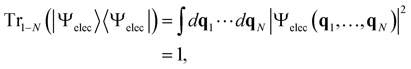 | (1) |
| Tr1−N(Ĥ(el)|Ψelec〉〈Ψelec|) = E, | (2) |
Then the charge density operator ![[small rho, Greek, circumflex]](https://www.rsc.org/images/entities/i_char_e0b7.gif) is defined as
is defined as
|
NTr2−N(|Ψelec〉〈Ψelec|) = ,
| (3) |
|
Tr1 = N.
| (4) |
Löwdin13 (see also ref. 14) defined the natural orbitals (NO) |λk〉 as eigenfunctions of such that
|
|λk〉 = nk|λk〉,
| (5) |
2.2 Intrinsic energetic structure of electronic states
We seek for the information content about the electronic energy. A straightforward extension of the charge density to the energy domain is defined as| Tr2−N(Ĥ(el)|Ψelec〉〈Ψelec|) = Ĥ(1), | (6) |
| Tr1Ĥ(1) = Tr(Ĥ(el)|Ψelec〉〈Ψelec|) = E. | (7) |
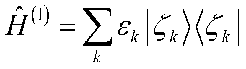
Since 〈r|Ĥ(1)|r〉 is an energy density distribution at point r, Ĥ(1) is appropriately called the energy density operator. It is also natural to extract the eigenfunctions and eigenvalues from Ĥ(1) such that
| Ĥ(1)|ζk〉 = εk|ζk〉. | (8) |
We call |ζk〉 the Energy Natural Orbitals (ENOs),2 and they are ortho-normalized to unity, satisfying
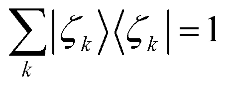 | (9) |
| 〈ζl|ζk〉 = δlk. | (10) |
By definition, the sum of all the eigenvalues is equal to the total energy as
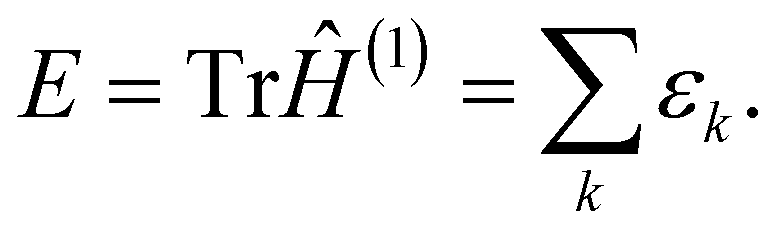 | (11) |
We define the population of each ENO, say ξk, as
|
ξk = 〈ζk||ζk〉.
| (12) |
Thus the set of energy and population of the ENOs gives an invariant internal structure of the total electronic energy E. Furthermore,
 | (13) |
Since the electronic Hamiltonian operator Ĥel can be decomposed into the electronic kinetic energy, the nuclear-electronic attraction, and the electron–electron repulsion terms, so can the one-electron operator Ĥ(1). Through such a decomposition, the energy components of the total correlated electronic wavefunction can also be determined.
2.3 Transformation to the sound
To make it possible for ENOs to be audible, a given ENO energy range [ε1, ε2] is linearly mapped to a frequency range [f1, f2],
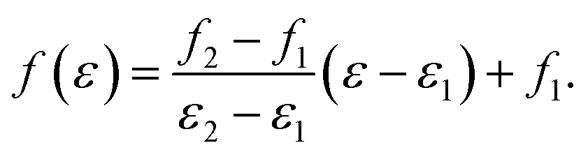 | (14) |
Then the amplitude of sound may be given as
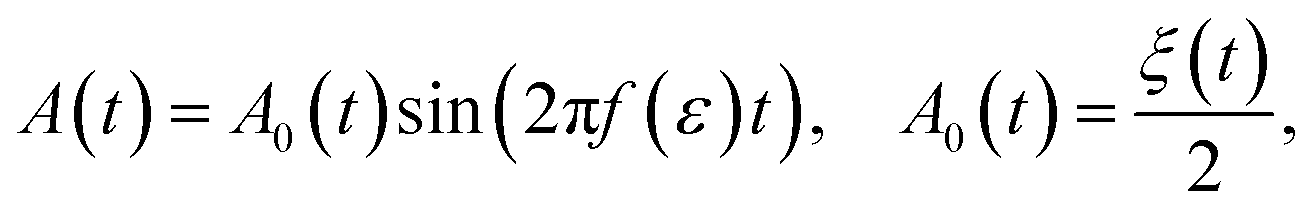 | (15) |
Because the energy is time-dependent, a straightforward implementation of eqn (15) would result in unwanted chirp. The frequency may be kept constant for a short interval, such as a single cycle, so that the sound intuitively corresponds to the energy it is supposed to represent. The human ear has different responsiveness to different frequency ranges. Some frequency-dependent adjustments to the volume may be necessary for best reception.
Since the energy range depends on interest and can vary greatly, there is no single mapping to frequency that meets all needs. In the examples below, some suggestions are made, such as assigning notes to atomic energy for dissociation, or including only the most significantly interacting ENO energies in a convenient frequency range.
We herein present several examples of molecular sound in multimedia files given as ESI.† The files include the following clips, which are explained in detail in the following sections.
(1) H2 11Σ+g bond formation, in the ENO representation (ESI† file: clip1.mp4).
(2) H2 21Σ+g bond formation, in the ENO representation (ESI† file: clip2.mp4).
(3) LiF singlet ground state dissociation (ESI† file: clip3.mp4).
(4) LiF singlet first excited state dissociation (ESI† file: clip4.mp4).
(5) B12 highly excited state adiabatic dynamics with a dissociating atom (ESI† file: clip5.mp4).
The multimedia presentations prepared for this paper linearly scale down the amplitude of higher frequencies. The measures actually taken for the ESI† multimedia presentations to adjust to the human ear are outlined in the Appendix.
3 Formation of a hydrogen molecule
We begin the sonic representation with the bond formation of a hydrogen molecule from two H atoms in the ground state.43.1 Computational level
The three lowest singlet states of H2 were computed in a previous work,4 employing full configuration interaction with the aug-cc-pVQZ basis set (92 molecular orbitals with 674 and 628 configurations for 1Σ+g and 1Σ+u, respectively). All quantum chemistry calculations in this paper are done with the GAMESS quantum chemistry package.15The resulting potential energy curves are shown in Fig. 1 with further description given in the following subsections.
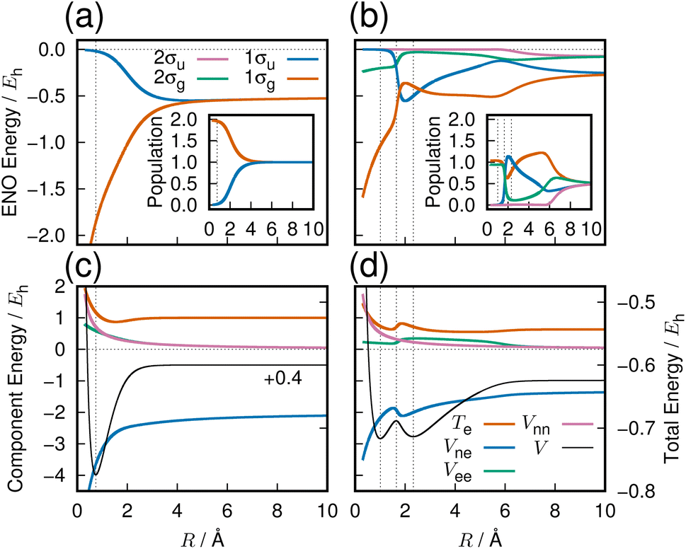 | ||
| Fig. 1 Ground and first excited singlet gerade states of H2. Panels (a) and (b): the ENO energy curves for the states 11Σ+g and 21Σ+g, respectively. The inset in each shows the ENO population curves. ENOs with essentially zero population everywhere are omitted from the figure. The color key to the curves is given in panel (a). Panels (c) and (d): the total electronic potential energy curves (V, black, scales to the right) for the states corresponding to the panels in the top row, and its components (scales to the left), electronic kinetic energy (Te, orange), nuclear-electronic attraction energy (Vne, blue), electron–electron repulsion energy (Vee, green), and nuclear–nuclear repulsion energy (Vnn, pink). The color key to the curves in (c) and (d) are shown in panel (d). The 11Σg potential energy curve is vertically raised by +0.4Eh to place it in the same range as the excited state curve. Dotted vertical lines indicate potential minima and maxima. | ||
3.2 Sound of formation of a hydrogen molecule in the ground state
To map the energy into the audible frequency range, we take the range −0.5Eh through 0Eh as the frequency of the notes A4 through C5# (where A and C represent the note and the following number gives the octave, in the scientific pitch notation) (see Table 1). The choice places the lower note C3 at an energy of −1.852Eh, so that the energy range represented in Fig. 1(a) and (b) is conveniently within auditory range. The volume of the sound is given proportional to the population of each ENO.
| Energy (Eh) | Frequency (Hz) | Note |
|---|---|---|
| 0.000 | 1108.7 | C5# |
| −0.136 | 1046.5 | C5 |
| −0.500 | 880.0 | A4 |
| −1.280 | 523.3 | C4 |
| −1.462 | 440.0 | A3 |
| −1.852 | 261.6 | C3 |
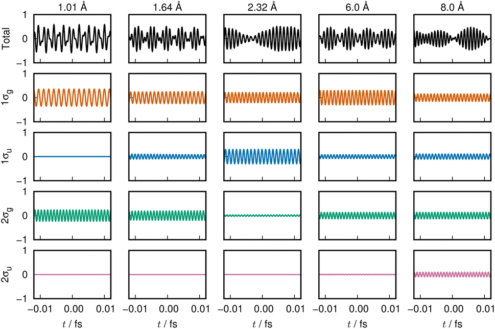
The variation of the 1σg ENO and 1σu ENO with respect to the internuclear distance R are audible, respectively, in Clip 1a and Clip 1b in the ESI† multimedia file clip1.mp4, and the combined sound is heard in Clip 1c in the same file. The smooth transition is reflected in the sounds. In Fig. 2, the sound (voiceprint) at the internuclear distances R = 0.74, 3.0, and 6.0 Å are shown as waveforms.
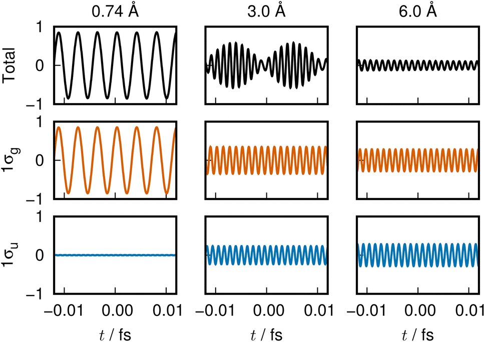 | ||
| Fig. 2 Voiceprint of the 11Σ+g state. From left to right, the sounds at R = 0.74, 3.0, and 6.0 Å, respectively, are shown as waveforms. The total signal and the sounds from the 1σg ENO (orange) and 1σu ENO (blue) are shown from the top to bottom. | ||
Both the 1σg ENO and the 1σu ENO at large R correlate to the same H-atom energy with a population of one, but the 1σu population transfers to the 1σg ENO as R approaches Re, with the 1σu ENO energy going to zero. Thus we see a smooth transition from the valence-bond-like (atomistic) to the molecular-orbital-like (molecular) state naturally represented with ENOs. At a long distance (6.0 Å), the two ENOs are degenerate in energy, giving out the same sound. Coming closer to a distance of 3.0 Å, the 1σg ENO heads toward lower energy, with its population increasing at the same time, while the 1σu ENO heads toward higher energy with decreasing population. The slightly differing frequencies from the two result in an audible beating pattern. When R approaches Re, the sound from 1σu, with its zero population, is no longer heard, whereas the sound from 1σg is now of a low frequency, signifying low electronic energy. Together with the nuclear–nuclear repulsion energy (not heard), the minimum at Re is made.
The sound from the 1σg ENO keeps lowering, reflecting the fact that its energy gets monotonically lowered. The volume of its sound becomes larger at R shorter than about 4.0 Å due to the increase of the population from 1.0 to 2.0 at the end. On the other hand, the sound from the 1σu ENO rises as R becomes shorter. The most striking impression from its sound is that the volume diminishes to zero as it nears the minimum at Re. The complicated sound from the total state (combined 1σg ENO and 1σu ENO) therefore gets simpler, heard only from the 1σg ENO.
Our observation based on ENO analysis is as follows (see also Fig. 1(a) and (c)). As R becomes shorter, the bond formation proceeds as follows:4
(1) The entire feature of the electronic energy is dominated by two major ENOs only: 1σg and 1σu (Fig. 1(a)).
(2) At very large values of R, the sounds of 1σg and 1σu are mutually the same and set to that of the 1s orbital of the hydrogen atom.
(3) The significant interaction between the two H atoms begins from about 6 Å, where the beat between the sounds of 1σg and 1σu begins to be heard.
(4) Vee and Vnn keep increasing monotonically, while Vne comes downslope monotonically and more extensively.
(5) As seen in Fig. 1(c), which has been based on a very accurate electronic wavefunction as a function of R, Te begins to decrease at about 3 Å, hitting the bottom at 1.5 Å, and rises through the equilibrium R distance (Re). The rise at Re is required by the virial theorem for the potential curve to make the bottom.
(6) As confirmed in Fig. 1(c), it is only Vne that can lower the electronic energy significantly enough for bond formation. The constant lowering of Vne is realized practically only by the 1σg ENO (Clip 1a of the ESI† multimedia file clip1.mp4). It is natural, therefore, to conclude that the lowering of Vne is the predominant origin of the bond formation. Note that the lowering of Vne has come as a consequence of electronic-state reorganization from the atomic to covalent states, and therefore it is not a result of classic electrostatic interactions alone.
Our ENO analysis is simpler and invariant in that any chemists applying any accurate electronic wavefunctions should reach the same and unique conclusion. But it seems not precise enough to support the Ruedenberg theory. Yet there are two comments: the kinetic energy lowering seen in Fig. 1(c) is simply due to the dramatic decreasing of the population of the 1σu ENO, which has a high kinetic energy (accompanying that, the 1σu ENO energy approaches zero as R nears the Re (the reader is referred to Clip 1b in the ESI† multimedia file clip1.mp4). On the other hand, near Re, Te rises as R becomes shorter, which is consistent with the virial theorem.4 The numerical analysis reveals that Te of the 1σg ENO keeps increasing all the way through R with no stage of lowering, as R becomes shorter. It turns out, therefore, that the electronic kinetic energy of bonding for the 1σg ENO does not experience lowering. We therefore may rather say that the electrons come to be confined in the bonding area due to covalency, contrary to the assertion by Hellmann. We are interested in the possible sound from the Ruedenberg's contraction of the atomic orbital.16 However, we need additional ideas to make it possible to be audible as a simulation of a physical process.
3.3 Sounds from the 21Σ+g state of a hydrogen molecule
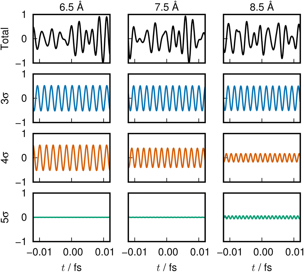
We next sample from the bond formation of the 21Σ+g state of a H2 molecule. Although more complicated than the 11Σ+g state, only 4 ENOs are found to essentially dominate the state. Their energy variations along R are displayed in Fig. 1(b), with the inset showing the associated populations. Fig. 1(d) shows the potential energy curve V (black curve), Te, Vne, Vee, and Vnn. There exists a double minima in this state at RL = 1.007 Å and RR = 2.323 Å, and a single peak in between at RS = 1.642 Å, as seen in Fig. 1(d), which demonstrates that the 21Σ+g state appears to be a class of the forbidden reaction in contrast to the 1Σ+g state. The condition for the potential basin and summit (barrier) to be formed was clarified in terms of the adiabatic virial theorem.4 Vne decreases monotonically up to a point near the right minimum as R becomes shorter, then rises in the vicinity of the position of the summit and decreases further to the left of the summit and beyond. Te is seen to make a shallow and wide basin towards the right of RR, thereby giving a peak, which comes down to another basin as R becomes shorter. Vee produces a plateau in the range of 2.0 < R < 7.0 Å.It turns out that at the longer distance local minimum RR = 2.323, the energy density is composed mainly of the 1σg ENO and the 1σu ENO, while the minimum at RL = 1.007 Å is given by the 1σg ENO and the 2σg ENO (note that both 1σg and 1σu of the 21Σ+g state are different from those of the 11Σ+g). The roles of 1σu and 2σg interchange drastically around the summit of the potential barrier in between. 2σu loses its role in the very early stage (at long R). Incidentally, the appearance of the 1σu ENO in the 1Σ+g comes from the configuration of double occupation in the 1σu ENO, and this is why we refer to this bond formation as a prototype of the forbidden reaction. One can dynamically experience the interchange between the roles of 1σu and 2σg ENOs by hearing the sound of them: 1σu in Clip 2b and 2σg in Clip 2c in the ESI† multimedia file clip2.mp4. In contrast, by hearing the sound of 1σg (Clip 2a), we vividly understand that the 1σg ENO constantly supports the chemical bond throughout R, although the variation in its sound is not monotonic in contrast to the 1σg of the 11Σ+g state. The combined sound of all these components can be heard in Clip 2d,† which demonstrates how a complicated two-electron process is involved in the formation of this chemical bond. The voiceprints of this system are sketched in Fig. 3.
 | ||
| Fig. 3 Voiceprint of the 21Σ+g state, drawn in the same manner as in Fig. 2. | ||
4 The avoided crossing: LiF
4.1 Computational level
To demonstrate the potential of sonification in nonadiabatic chemistry, we take the well-known avoided crossing between the lowest two adiabatic 1Σ+ states of the LiF molecule, which we call states S1 and S2. Accurate potential curves obtained by state-averaged CASSCF orbital determination followed by multireference configuration-interaction, employing basis sets up to the complete basis-set limit have been reported in the literature.22,23 For a demonstration of the voiceprint in the study of the avoided crossing between S1 and S2 only, a much simpler description computed in a previous study,2 of 2-states averaged, 8 electrons in 7 orbitals CASSCF followed by a single reference singles and doubles configuration interaction (lowest three orbitals frozen) with the small cc-pVDZ basis set,24,25 is adequate. Here again the GAMESS program has been utilized.15 The basis set includes 3 sets of s functions, 2 sets of p functions, and a set of d functions on each atom, resulting in 12 σ orbitals, 12 π orbitals, and 4 δ orbitals.4.2 Global energetic feature of the lowest avoided crossing of LiF
Fig. 4(a) exhibits the global feature of the electronic energies of the adiabatic ground state S1 and the first excited state S2. The inset expands the avoided crossing region between the two potential energy curves. We will focus on giving an auditory representation of the avoided crossing within the range of internuclear distances 6–9 Å. | ||
| Fig. 4 (a) Lowest singlet LiF potential curves V1 and V2 for the states S1 and S2, respectively. The inset shows the avoided crossing enlarged. (b) The ENO energy for the S1 state, and (c) for the S2 state. The lowest non-core σ orbitals and a π orbital are shown. (d) The ENO population for the S1 state and (e) for the S2 state. ENOs 2σ and 1π have population of 2.0 and are not shown in the lower panels. | ||
4.3 Sonic description of the avoided crossing
The energy of the dominant ENOs around the avoided crossing are shown in Fig. 4(b) and (c), for the states S1 and S2, respectively. Plotted are the lowest five σ ENOs except for the core 1σ ENO (2σ through 6σ), and also the first π ENO. All the other ENOs have an energy and population close to zero and are omitted in the figure. ENO populations of the three orbitals 3σ, 4σ, and 5σ, which vary significantly around the avoided crossing, are shown in Fig. 4(d) and (e) for the states S1 and S2, respectively. The population of the 1σ, 2σ, and 1π ENOs is 2.0 in the same region.A fuller description in terms of ENO was given previously,2 and we here repeat the most significant findings to illustrate the utility of their sonic representation. The present nonadiabatic electron transfer seems overwhelmingly dominated by the three ENOs 3σ, 4σ and 5σ, as demonstrated in Fig. 4. Note that the interaction between them reflects the electron transfer within the molecule. For the S1 state, the “covalent” configuration with two electrons in the 4σ ENO for shorter internuclear distance becomes the “ionic” configuration at longer internuclear distance with one electron each in the 4σ and 5σ ENOs. The S2 state configuration is nearly a mirror image of the S1 state.
A huge energy change is noted for some ENOs in Fig. 4(b) and (c); for instance, ENO 4σ in S1 (panel (b)) drops (becomes more stable) more than 2 hartrees (Eh) by the transition from the distance R = 8 to 7 Å, and the steep rise of ENO 4σ is seen in panel (c) for the S2 state. This drastic variation in energy happens because the ENOs are population dependent.
Table 2 shows the chosen mapping of the energy range to the audible frequency. The mapping is so that the 2σ energy is represented with a C3 sound, the 3σ and 4σ are roughly an octave higher, and 5σ is roughly another octave higher.
| Energy (Eh) | Frequency (Hz) | Note |
|---|---|---|
| 0.000 | 924.0 | |
| −0.779 | 880.0 | A4 |
| −7.097 | 523.3 | C4 |
| −8.572 | 440.0 | A3 |
| −11.731 | 261.6 | C3 |
In the graphs of the population variation, Fig. 4(d) and (e), the 5σ ENO seems to play a major role in the change of electronic character across the avoided crossing, both in the S1 and S2 states. Meanwhile the variation of the 3σ ENO seems small both in energy and population. However, it turns out that the 3σ and 4σ ones are the dominant players in the present avoided crossing. Listen to the sounds:
For the S1 state, 3σ ENO in Clip 3a in the ESI† multimedia file clip3.mp4; 4σ in Clip 3b; and the combination of three ENOs, 3σ, 4σ, and 5σ, in Clip 3c.
For the S2 state, 3σ in Clip 4a of the file clip4.mp4; 4σ in Clip 4b; and the combined one in Clip 4c.
The sounds of 3σ and 4σ along with the variation of their spatial distributions (and 5σ as well) in the S1 and S2 states highlight the very clear symmetric exchange of their roles across the avoided crossing. The voiceprints are also presented graphically in Fig. 5 for the S1 state and Fig. 6 for the S2 state. A large variation in the 4σ ENOs in S1 and S2 before and after the avoided crossing are noted. It turns out that the 5σ ENO plays an auxiliary role to the interchange of the roles of the 3σ and 4σ ENOs.
 | ||
| Fig. 5 LiF S1 state voiceprint, shown in the same manner as in Fig. 2. Significant change in the 4σ and 5σ sound is heard across the avoided crossing. | ||
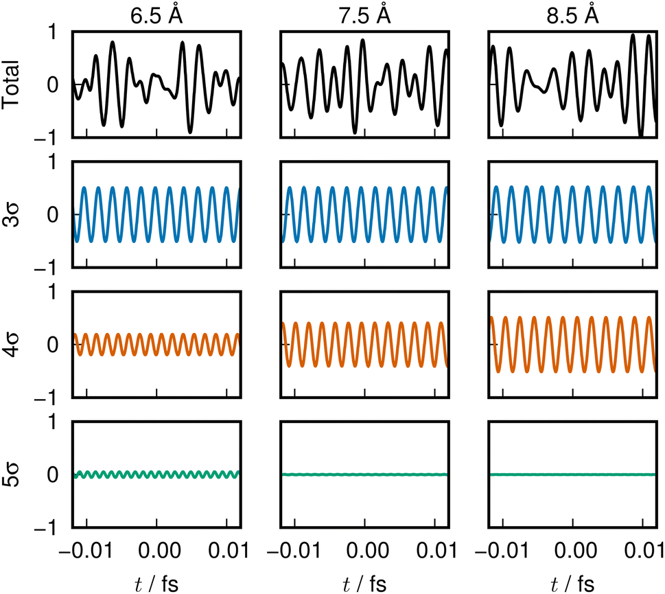 | ||
| Fig. 6 LiF S2 state voiceprint, shown in the same manner as in Fig. 2. It is nearly a mirror image of the S1 voiceprint for the range near the avoided crossing. | ||
5 Cluster dynamics in a highly excited electronic state: B12
The last example is taken from an ab initio MD dynamics simulation of molecular dissociation in the densely quasi-degenerate electronic state manifold of B12 clusters.26,27 The many vacancies in the 2p orbital valence space of the boron atoms give rise to the highly quasi-degenerate manifold of excited states, and for balance between their rough representation and computation-intensive dynamics, we choose to use the STO-3G minimum basis set for molecular orbital determination and configuration interaction singles and doubles from the highest occupied molecular orbital (HOMO) and HOMO−1 (MO 29 and 30) to all virtual orbitals for the excited states description. The number of configuration state functions included in the calculation is 1891.The excited states in such highly degenerate manifolds are generally of very long lifetime as discussed in a previous paper, due to what we call the intramolecular nonadiabatic electronic-energy redistribution (INER).27 Therefore, in order to study the dissociation dynamics for B12 → B11 + B, we need to find or intentionally prepare a moment right before a dissociation. Fig. 7 shows the time-variation of 60 ENOs on the occasion of such a dissociation, which starts at about 30 fs in the graph. Despite a very wild diffusive electronic wavepacket state in the Hilbert space,27 we find a very clear layer structure composed of 4 bands to exist before dissociation: the core layer (panel(c) in Fig. 7) composed of ENOs 1 through 12 of the lowest energy; the valence layer in panel (b) from ENOs 13 to 28; the half-occupied layer of ENOs 29 and 30 (panel (a), the lower part); and the flowing layer from ENOs 31 to 60 (panel (a), the upper band).
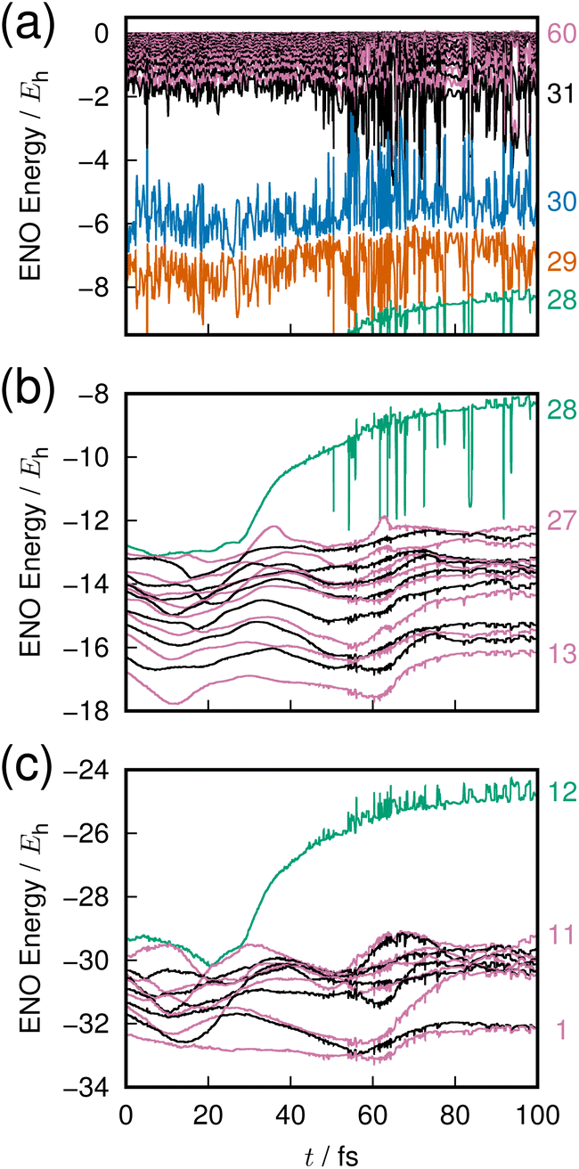 | ||
| Fig. 7 Adiabatic dissociation dynamics in an excited state B12 cluster, shown as time-evolution of the ENO energies. (a) Flowing and half-occupied layer ENOs. (b) Valence-layer ENOs. (c) Core-layer ENOs. Numbers on the far right label the selected ENOs. The highest ENO from the valence layer (#28) represents the dissociating atom. | ||
On the occasion of the dissociation, we find two irregular behaviors by one ENO of the core (ENO 12, panel (c), green) and by another of the valence layer (ENO 28, panel (b), green). The other ENOs seem rather stable, but we see that violent large-amplitude oscillatory behavior follows the two precursors' quick rise of the two ENOs. Let us hear the sound of these two ENOs.
The chosen mapping of energy to sound in the present paper for the B12 cluster is given in Table 3. Because of the many ENOs involved, a simple superposition of the sounds of all the ENOs results in apparent noise. It is more rewarding to focus on a subfeature.
| Energy (Eh) | Frequency (Hz) | Note |
|---|---|---|
| 0.094 | 1046.5 | C5 |
| −6.993 | 880.0 | A4 |
| −22.178 | 523.3 | C4 |
| −25.721 | 440.0 | A3 |
| −33.314 | 261.6 | C3 |
In Clip 5a of the ESI† multimedia file clip5.mp4, we pick out the sound of ENO 12 only. A very quick rise of the pitch is heard, which was made possible by singling out the ENO. Indeed, it is not well distinguished in the combined sounds over the core layer, Clip 5b. A similar procedure is undertaken for ENO 28 (Clip 5c) and the valence layer (Clip 5d). In the combined sound in the half-occupied (Clip 5e) and flowing layers (Clip 5f), we notice a larger fluctuation in the sound after time t = 50 fs, around which the violent oscillation begins to be seen. In Clip 5g, sounds from all the combined ENOs are present, which sound like a noise. Yet, we can notice the moment that one boron atom departs from the mother cluster. The voiceprints for the relevant ENOs at selected times are recorded in Fig. 8.
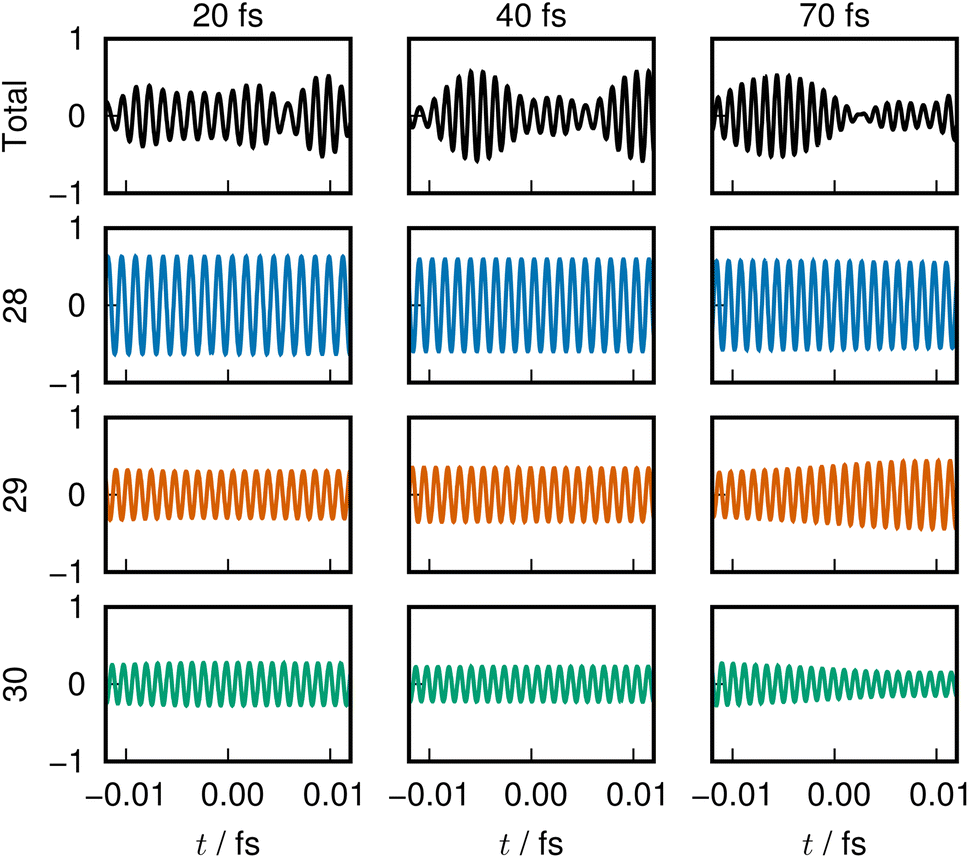 | ||
| Fig. 8 Sound from adiabatic dissociation from a B12 cluster, presented in a similar manner as in Fig. 2. The dissociation is associated with rising energy of the 28th ENO, which is reflected in its sound. | ||
Obviously, the present sound analysis is not sufficient to identify the mechanical roles of these specific ENOs in the dissociation dynamics, and further analysis is needed.
6 Concluding remarks
We have shown that the energy natural orbital analysis has made sonification of the molecular electronic energy density possible. Since the total electronic energy E(R) at a given nuclear configuration (R) is represented as an exact sum of the ENO energies such that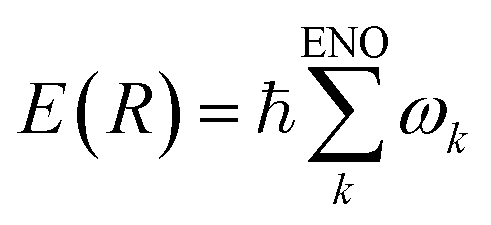 , {ωk} values are linearly transformed into the audible frequency range {fk}. The amplitude of each frequency is modulated by the population of the relevant ENO, and thereby the pitch and volume pair due to each ENO give rise to an audible sound. The sum over all of them, a polyphonic sound, brings about a total voiceprint, characterizing the rich energetic structure forming the molecule. It should be stressed that the relevant sonification can be applied not only to the ground state but to the excited and wavepacket ones. The procedure is valid at any molecular configuration and therefore sonification of the electronic dynamical process of chemical reactions can also be achieved.
As the first example of the molecular electronic energy sound, we have shown rather simple and straightforward applications to chemical bonding of a hydrogen molecule, the avoided crossing in LiF, and quantum electron wavepacket dynamics in the highly excited state of a boron cluster.
In the formation of a hydrogen molecule in the 11Σ+g state, the beat arising from the combined sounds of the 1σg ENO and the 1σu ENO was highlighted as an early interaction of two hydrogen atoms. Moreover, it has been stressed that the decreasing population of the 1σu ENO toward the bond formation is heard as the diminishing (fainting) of its sound. The strange behavior of the total electronic kinetic energy in the course of bond formation, the interpretation of which had been a cause of controversy in the past, turns out to be due to this diminishing.
A hydrogen molecule in the 21Σ+g state represents a typical situation, so to speak, of the forbidden reaction, and has two local minima separated by a potential barrier. It turns out that the potential basin at the longer nuclear distance is formed by the pair of the 1σg ENO and the 1σu ENO, while that of the shorter distance is due to the set of the 1σg ENO and the 2σg ENO. Therefore, the sound of 1σu disappears before the potential barrier and the sound of the 2σg ENO begins to be appreciated after the barrier.
Likewise, the passage across the avoided crossing in LiF can be clearly distinguished with just the three tones coming from the 3σ, 4σ, (and 5σ) ENOs. Also in the dissociation event in the B12 cluster, the sound from only a couple of ENOs are heard to surge quickly.
The sounds mentioned above are all simple and rather primitive in that only direct “sound” of the single ENO and the total sum thereof are heard. The method of sonification need not be as simple nor unique, and methods other than those presented in this paper are possible. For instance, we could have artificially overlaid overtones in specific ways to the sound of each ENO, with which we can mimic the sound of musical instruments like the violin, oboe, and so on. Such an articulation should facilitate distinguishing the individual tones in the total mixture.
The sonification of molecular states is a matter of representation or presentation, and is in the secondary stage of the progress in quantum chemistry, viewing from the zeroth-order efforts for solving and/or integrating the Schrödinger equation. We believe though that the advent of Natural Orbitals (NOs) followed by the development of ENOs have succeeded in bringing out the exact one-electron pictures of the electron density and electronic-energy density, respectively, from the very complicated many-body electronic wavefunctions. Understanding in the one-electron picture should be indispensable in the deeper understanding and prediction of chemical phenomena. The sound information is hence a subsidiary, yet necessary, outcome from the ENO studies.
Just as with visualization technology for molecular electronic states, the sonification of electronic energy structures could be a useful tool that is vividly appealing to another dimension of our sense perception. In particular, the hearing experience offers the immersive feeling of dynamics in terms of the time variation of high-and-low pitch, dynamical range (variation of the sound volume), beat (interference) among the adjacent frequencies, and so on. These should add an additional excitement in chemical research. Now that a direct route of access to the sound of electronic energy has been opened, the progress of the general sonification technology1,12 by its own virtue, such as sophisticated methodology with artificial intelligence (AI), should enhance our (sensory and/or intuitive) understanding of molecular electronic energy states and chemical reactions. Among other subjects, we are interested in the sound representation of the dynamics of:
(1) spin-current dynamics in open-shell systems described by the energy natural spin orbitals (ENSO), in which different spins are supposed to make different sounds;28,29
(2) electronic energy current from the nonadiabatic electron wavepacket dynamics in the highly excited state manifold, and other electronic energy flows in the real-time dynamics of the Förster fluorescence resonance energy transfer;30
(3) electronic state avalanche after making a hole in the core (like the 1s state) of a molecule; the avalanche of which is supposed to lead to autoionization;31
(4) distinction of allowed (cooperative) and forbidden reactions in the excited-state chemistry, and so on.
To conclude, we emphasize again that the sound representation of the molecular electronic energy density is an outcome of the representation in Energy Natural Orbitals, since its energy and population can be qualitatively expressed at a time. Each ENO can be regarded as a string (actually many-dimensional) of a musical instrument such as a harp. Yet, one of the inherent characteristics of this instrument is that the sound pitch (energy) and the volume (population) of each string (ENO) can dynamically vary according to the change in the molecular states and geometry, which is particularly useful in the study of chemical reactions and electronic excited states. In addition, recall that ENOs are exact if the mother electronic wavefunction is exact and there is no room for subjective articulation to take part. Therefore, ENO and its sonification can be utilized as promising tools in molecular electronic state theory.
Appendix
A Adjustments in transforming molecular frequency to audible frequency
As outlined in Section 2.3, the linear mapping from molecular frequency to audible frequency was further adjusted for the human ear in the ESI† multimedia presentations.Because human hearing is much more sensitive at higher frequencies than lower ones within the range 100–1000 Hz, we linearly adjust the maximum amplitude A0 in eqn (15) determined by the ENO population (or taken to be constant for energy-component-based voiceprints) as
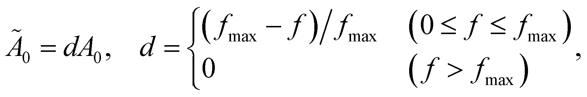 | (16) |
A straightforward implementation of eqn (15) results in unintuitive chirping because the frequency of sound is time dependent. We keep the frequency within a cycle constant in the following manner, to avoid such unwanted effects, so we may rewrite the amplitude of sound as a sequence of cycles:
|
A(t) = Ã0sin(2π(t − t0)f) = Ã0sin(2π(τ + h)),
| (17) |
| τ = ⌊(t − t0)f⌋, 0 ≤ h < 1, | (18) |
| sin(2π(t − ta)f(ta)) = 0, τa = ⌊(t − t0)f(ta)⌋, | (19) |
Conflicts of interest
There are no conflicts to declare.Acknowledgements
This work is dedicated to two quantum chemists who are visually impaired. The work has been supported by JSPS KAKENHI, Grant No. JP20H00373.Notes and references
- T. Hermann, A. Hunt, J. G. Neuhoff, et al., The Sonification Handbook, Logos Verlag Berlin, 2011, vol. 1 Search PubMed.
- K. Takatsuka and Y. Arasaki, J. Chem. Phys., 2021, 154, 094103 CrossRef CAS PubMed.
- K. Takatsuka and Y. Arasaki, J. Chem. Phys., 2021, 155, 064104 CrossRef CAS PubMed.
- Y. Arasaki and K. Takatsuka, J. Chem. Phys., 2022, 156, 234102 CrossRef CAS PubMed.
- T. Fujimoto and Y. Takahashi, The 17th Annual Conference of the Japanese Society for Artificial Intelligence (in Japanese), 2003 Search PubMed.
- R. Miura, Y. Ando, Y. Hotta, Y. Nagatani and A. Tsuda, ChemPlusChem, 2014, 79, 516–523 CrossRef CAS PubMed.
- B. Mahjour, J. Bench, R. Zhang, J. Frazier and T. Cernak, Digital Discovery, 2023, 2, 520–530 RSC.
- S. Nakamura, Chem. Today, 2012, 494, 39 CAS.
- P. G. Szalay, T. Müller, G. Gidofalvi, H. Lischka and R. Shepard, Chem. Rev., 2012, 112, 108–181 CrossRef CAS PubMed.
- T. Helgaker, S. Coriani, P. Jørgensen, K. Kristensen, J. Olsen and K. Ruud, Chem. Rev., 2012, 112, 543–631 CrossRef CAS PubMed.
- H. Lischka, D. Nachtigallová, A. J. A. Aquino, P. G. Szalay, F. Plasser, F. B. C. Machado and M. Barbatti, Chem. Rev., 2018, 118, 7293–7361 CrossRef CAS PubMed.
- G. Kramer, B. Walker, T. Bonebright, P. Cook, J. H. Flowers, N. Miner and J. Neuhoff, Sonification Report: Status of the Field and Research Agenda, Department of Psychology, University of Nebraska technical report, 2010 Search PubMed.
- P.-O. Löwdin, Phys. Rev., 1955, 97, 1474–1489 CrossRef.
- E. R. Davidson, Rev. Mod. Phys., 1972, 44, 451–464 CrossRef CAS.
- M. W. Schmidt, K. K. Baldridge, J. A. Boatz, S. T. Elbert, M. S. Gordon, J. H. Jensen, S. Koseki, N. Matsunaga, K. A. Nguyen, S. Su, T. L. Windus, M. Dupuis and J. A. Montgomery Jr, J. Comput. Chem., 1993, 14, 1347–1363 CrossRef CAS.
- K. Ruedenberg, Rev. Mod. Phys., 1962, 34, 326–376 CrossRef CAS.
- M. S. Gordon and J. H. Jensen, Theor. Chem. Acc.: New Century Issue, 2001, pp. 248–251 Search PubMed.
- R. F. Bader, J. Phys. Chem. A, 2011, 115, 12667–12676 CrossRef CAS PubMed.
- G. B. Bacskay and S. Nordholm, J. Phys. Chem. A, 2017, 121, 9330–9345 CrossRef CAS PubMed.
- D. S. Levine and M. Head-Gordon, Nat. Commun., 2020, 11, 4893 CrossRef CAS PubMed.
- H. Hellmann, Z. Phys., 1933, 85, 180–190 CrossRef CAS.
- T. J. Giese and D. M. York, J. Chem. Phys., 2004, 120, 7939–7948 CrossRef CAS PubMed.
- A. J. C. Varandas, J. Chem. Phys., 2009, 131, 124128 CrossRef CAS.
- T. H. Dunning Jr, J. Chem. Phys., 1989, 90, 1007–1023 CrossRef.
- B. P. Prascher, D. E. Woon, K. A. Peterson, T. H. Dunning and A. K. Wilson, Theor. Chem. Acc., 2011, 128, 69–82 Search PubMed.
- Y. Arasaki and K. Takatsuka, J. Chem. Phys., 2023, 158, 114102 CrossRef CAS.
- K. Takatsuka and Y. Arasaki, J. Chem. Phys., 2023, 159, 074110 CrossRef CAS.
- K. Hanasaki and K. Takatsuka, Chem. Phys. Lett., 2022, 793, 139462 CrossRef CAS.
- K. Hanasaki and K. Takatsuka, J. Chem. Phys., 2023, 159, 144111 CrossRef CAS PubMed.
- K. Takatsuka and Y. Arasaki, J. Chem. Phys., 2022, 157, 244108 CrossRef CAS.
- T. Matsuoka and K. Takatsuka, J. Chem. Phys., 2018, 148, 014106 CrossRef.
Footnotes |
| † Electronic supplementary information (ESI) available. See DOI: https://doi.org/10.1039/d4ra00999a |
| ‡ Herman1 stated that “Sonification conveys information by using non-speech sounds. To listen to data as sound and noise can be a surprising new experience with diverse applications ranging from novel interfaces for visually impaired people to data analysis problems in many scientific fields”. |
| This journal is © The Royal Society of Chemistry 2024 |