
 Open Access Article
 This Open Access Article is licensed under a Creative Commons Attribution-Non Commercial 3.0 Unported Licence
Spectraformer: deep learning model for grain spectral qualitative analysis based on transformer structure
Zhuo Chenab,
Rigui Zhou *ab and
Pengju Renab
*ab and
Pengju Renab
aSchool of Information Engineering, Shanghai Maritime University, Shanghai, 201306, China. E-mail: rgzhou@shmtu.edu.cn
bResearch Center of Intelligent Information Processing and Quantum Intelligent Computing, Shanghai, 201306, China
First published on 7th March 2024
Abstract
This study delves into the use of compact near-infrared spectroscopy instruments for distinguishing between different varieties of barley, chickpeas, and sorghum, addressing a vital need in agriculture for precise crop variety identification. This identification is crucial for optimizing crop performance in diverse environmental conditions and enhancing food security and agricultural productivity. We also explore the potential application of transformer models in near-infrared spectroscopy and conduct an in-depth evaluation of the impact of data preprocessing and machine learning algorithms on variety classification. In our proposed spectraformer multi-classification model, we successfully differentiated 24 barley varieties, 19 chickpea varieties, and ten sorghum varieties, with the highest accuracy rates reaching 85%, 95%, and 86%, respectively. These results demonstrate that small near-infrared spectroscopy instruments are cost-effective and efficient tools with the potential to advance research in various identification methods, but also underscore the value of transformer models in near-infrared spectroscopy classification. Furthermore, we delve into the discussion of the influence of data preprocessing on the performance of deep learning models compared to traditional machine learning models, providing valuable insights for future research in this field.
1 Introduction
Grains, a fundamental source of human sustenance, are pivotal in agriculture and food security. This study explores advanced techniques in grain classification and quality assessment, which are crucial for enhancing agricultural productivity and ensuring food quality. While various grain types differ in morphology, chemical composition, and application, precise classification and assessment are key for optimizing production and supply chain efficiency. However, conventional methods are often time-consuming and complex, highlighting the need for improved approaches.We focus on three grains: barley, sorghum, and chickpeas. Each presents unique challenges in classification due to their visual similarities and diverse applications.
Barley, used in food, animal feed, and beer production, requires precise identification methods due to its visual similarity among varieties. While rich in starch, protein, and dietary fiber, its classification remains a time-intensive process, dependent on expert evaluation.
Chickpeas, high in protein and beneficial for soil health, face increasing challenges in variety differentiation due to growing seed similarities.1
Sorghum, versatile in food and biofuel production, necessitates accurate variety identification, particularly in livestock farming.2
Existing grain classification methods exhibit certain drawbacks. Firstly, many grain varieties bear an uncanny resemblance, confounding visual differentiation and thus fostering ambiguity and classification errors.
Secondly, prevailing classification methods often hinge on visual appraisal, rendering results susceptible to the evaluator's subjective judgment and experiential bias. Such subjectivity can engender disparate classification outcomes, diminishing the classification process's reliability and precision.
Moreover, the unique attributes of certain varieties may only become apparent in high-resolution images or under substantial magnification, amplifying the complexity and duration of the classification endeavor. These deficiencies underscore the difficulties inherent in current grain classification methodologies when confronted with varietal diversity and the imperative for precise identification. Consequently, the quest for more accurate and objective classification technologies becomes crucial to enhance efficiency and accuracy.
Near-infrared (NIR) spectroscopy3 is a non-destructive and rapid method for analyzing sample components, offering a simpler alternative to traditional chemical analysis by eliminating complex preparation like extraction or dilution. The NIR spectral region, typically spanning 780 to 2526 nm, aligns with the absorption of hydrogen-containing groups (O–H, N–H, C–H) in organic molecules. By scanning this region, NIR spectroscopy gathers characteristic information about these organic molecules.
A near-infrared spectrometer projects NIR light onto a sample, with different molecules absorbing light variably. NIR spectroscopy is non-destructive, efficient, and eco-friendly, offering speed, accuracy, and cost-effectiveness without chemical reagents. Traditional spectrometers, bulky and limited to labs, restricted NIR use in agriculture,4 food safety,5 and environmental monitoring,6 particularly for real-time analysis.7,8 Portable spectrometers, a notable advancement, allow for on-site, real-time NIR analysis but have a narrower spectral range, necessitating new methods for specific applications. Concurrently, advancements in computing and the internet have led to data abundance, fueling deep learning's expansion into various fields, including image and speech processing and natural language understanding.
As computer technology and computational capabilities have rapidly advanced and with the widespread adoption of the internet and other information technologies, large volumes of data have become easily accessible and storable. This data abundance has provided ample training samples for deep learning, which has found extensive applications across various domains, including image processing, speech recognition, and natural language processing.
In contrast to traditional machine learning approaches, deep learning algorithms can learn features directly from raw data through multi-layer automatic neural networks, eliminating the need for manual feature engineering. This simplifies the complexity associated with feature engineering and enables these models to capture intricate nonlinear relationships and patterns within the data.
In agriculture, the application of deep learning, particularly Convolutional Neural Networks (CNNs),9 in NIR spectroscopy has been demonstrated in recent studies. For instance, Yang et al.10 introduced the “TeaNet” method for classifying 50 black and green tea brands using NIR spectroscopy data. Their approach involved preprocessing the NIR spectroscopy data, transforming it into pseudo-images, and feeding it into a four-layer convolutional neural network, achieving an impressive classification accuracy of 99.2%. Similarly, Rong et al.11 proposed a seven-layer convolutional neural network model for categorizing five types of peaches based on VIS-NIR spectroscopy. Their model achieved a validation dataset accuracy of 100% and a test dataset accuracy of 91.7%. These examples highlight the increasing prevalence and success of CNNs in NIR applications in recent years.12–15
In the context of spectroscopic data, it is essential to recognize its inherent sequential nature, which significantly influences the predictive accuracy of models. Spectroscopic data often exhibits the repetition of spectral features at various positions, carrying similar information. However, in the feature extraction stage, CNNs typically excel at capturing local features.16 Still, they may need to pay more attention to global positional information, potentially leading to a failure in fully capturing the correlations between wavelengths. Consequently, despite identical spectral features at different positions, traditional CNNs struggle to establish connections among them, resulting in information loss.
To address this challenge, introducing the transformer architecture has proven to be a highly effective strategy.17 The transformer's attention18,19 mechanism assigns varying weights to features at different positions, enabling the model to prioritize crucial wavelength positions effectively. By learning and incorporating correlations between positions, the attention mechanism facilitates capturing sequential features inherent in spectroscopic data.20–22 This significantly enhances the model's grasp of the data's sequential nature, improving predictive accuracy.
Furthermore, the adaptive nature of the attention mechanism allows it to adjust weights dynamically, enabling the model to accommodate varying levels of information at different positions. This adaptability proves particularly advantageous when dealing with noise or variations in spectroscopic data, as it enhances the model's robustness and reduces the impact of noise on predictive performance.
We aim to unlock the potential of this fast and non-invasive method for rapid and precise classification and identification of these grain varieties. In the case of barley, we employed data from 24 different varieties, encompassing ten distinct sorghum varieties, and referenced data from 19 chickpea varieties from existing research.23 It's crucial to underscore that each grain type possesses its distinct spectral characteristics, with these traits subject to variation based on differences in varieties, growth conditions, and chemical compositions.
The primary objective of this study is to utilize a portable near-infrared spectrometer to identify barley, chickpea, and sorghum varieties in Ethiopia. Our secondary aim centers on exploring the potential of constructing a high-performance grain species recognition model by integrating near-infrared spectroscopy with transformer-based deep learning techniques. The third objective involves a comprehensive examination of the role of attention mechanisms in handling near-infrared spectroscopy data. Lastly, we undertake a comparative evaluation of different preprocessing techniques to identify the most suitable algorithm.
2 Materials and methods
2.1 Sample preparation
The collection and preparation of grain samples were conducted in Ethiopia by the Ethiopian Institute of Agricultural Research (EIAR) in June 2017.23 We utilized datasets for barley, chickpeas, and sorghum.† A total of 50 samples were collected for each variety, resulting in 24 barley varieties with a total of 1200 barley samples, 19 chickpea varieties with a total of 950 chickpea samples, and 10 sorghum varieties with a total of 500 sorghum samples. All these grains were produced in the same year to eliminate the influence of seed age.2.2 Portable near infrared spectrometer
The dataset was obtained using the SCIO Consumer Edition, a spectrometer designed by Consumer Physics for everyday use. It functions through a smartphone application and requires an internet connection to upload spectral data to a remote server. This device effectively covers a wavelength range from 740 to 1070 nanometers, including 331 unique variables.2.3 Spectral data preprocessing and data analysis method
Spectral data preprocessing is an essential step in spectral analysis, focusing on data quality enhancement through a series of sophisticated methods.24–26 This process commences with the optimization of the data's initial state, involving noise reduction and baseline adjustment. Subsequently, standardization is employed to ensure the data's uniformity and comparability, which is critical for the accuracy of further analyses and model development. In our methodology, we employed a diverse array of preprocessing techniques to refine raw spectral data.We employed the Savitzky–Golay smoothing technique (S) to effectively reduce random noise and achieve smoother spectral curves. Additionally, the AirPLS baseline correction method (A) was applied, which significantly minimized the influence of non-specific signals and improved the baseline quality of our data. To effectively counteract and eradicate any negative values found in our dataset, we deployed a targeted technique specifically designed for the removal of negative values (0). We standardized the data using the min–max normalization method (M), ensuring uniformity across a common scale and overcoming the challenges associated with varying units or ranges.
These preprocessing techniques were applied in various combinations, leading to a suite of methods: Savitzky–Golay smoothing (S), Min–Max normalization (M), Savitzky–Golay + AirPLS (SA), Savitzky–Golay + negativity removal (S0), negativity removal + Min-Max Normalization (0M), Savitzky–Golay + Min–Max normalization (SM), Savitzky–Golay + AirPLS + negativity removal (SA0), Savitzky–Golay + negativity removal + Min–Max normalization (S0M), Savitzky–Golay + AirPLS + Min–Max normalization (SAM), and Savitzky–Golay + AirPLS + negativity removal + Min–Max normalization (SA0M).
Post-implementation of these methods, we conducted a comparative performance analysis of five models, including the model proposed in this study, to develop a predictive model capable of identifying various grain classes. The evaluated models comprised a Support Vector Machine with a linear kernel (SVM (linear)),27 a Support Vector Machine with an RBF kernel (SVM (RBF)), a Random Forest algorithm (RF),28 a CNN, and our newly proposed spectraformer model. These models were assessed for their efficacy in analyzing preprocessed spectral data.
To develop a model boasting superior generalization capabilities, we implemented a 7![[thin space (1/6-em)]](https://www.rsc.org/images/entities/char_2009.gif) :3 ratio for training-to-testing data. Moreover, we incorporated a 5-fold cross-validation technique to enhance the model's robustness for more rigorous verification. This study leveraged a spectrum of machine learning algorithms, encompassing deep learning techniques, to delve into the relationship between spectral data and barley classifications. Fig. 1 meticulously delineates the data analysis workflow adopted in our research.
:3 ratio for training-to-testing data. Moreover, we incorporated a 5-fold cross-validation technique to enhance the model's robustness for more rigorous verification. This study leveraged a spectrum of machine learning algorithms, encompassing deep learning techniques, to delve into the relationship between spectral data and barley classifications. Fig. 1 meticulously delineates the data analysis workflow adopted in our research.
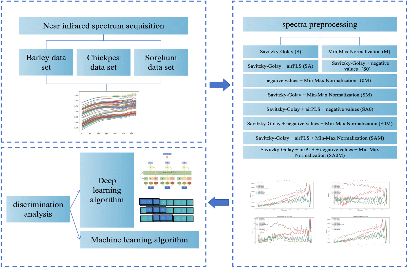 | ||
| Fig. 1 Flow chart of the data processing used. | ||
The challenge lies in precisely analyzing these short yet densely informative data sequences in spectroscopy. While CNNs excel in feature extraction and smoothing for one-dimensional data, they may face limitations when dealing with longer data sequences or the need to consider long-range dependencies. This limitation motivates the introduction of the transformer model.
Transformer models have already found wide-ranging applications in image processing and natural language processing domains.18,29–31 Therefore, this paper endeavors to introduce transformer modules into the field of spectroscopy. This effort seeks to leverage the powerful capabilities of transformers to enhance the efficiency of spectral data analysis and processing. By incorporating this advanced deep learning technology into spectroscopy research, the aim is to provide scientists with more accurate and efficient tools, ultimately fostering further development and innovation within the spectroscopy field. Fig. 2 visually illustrates the schematic structure of the transformer model, emphasizing its attention mechanism when processing sequential data.
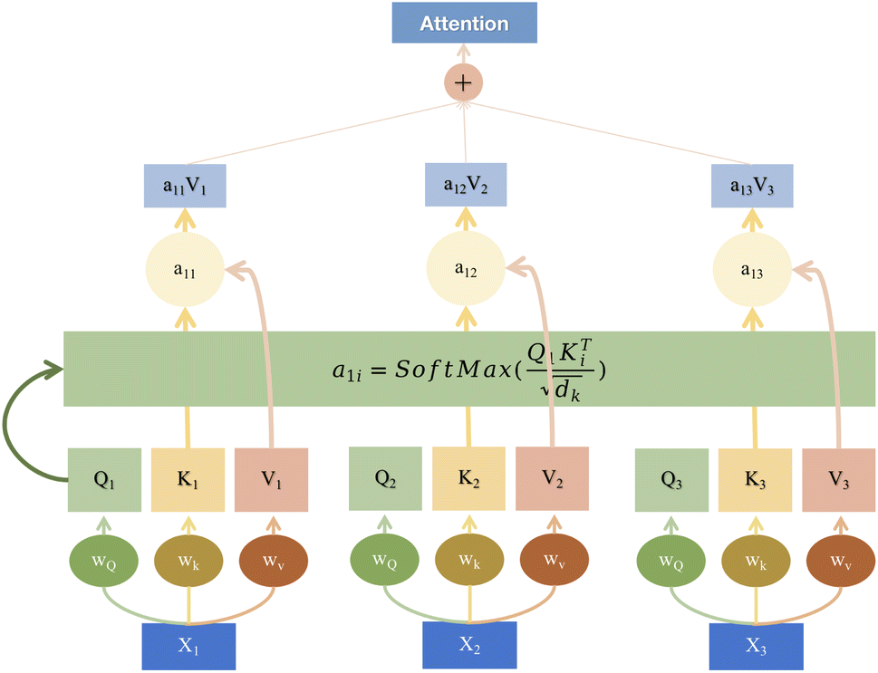 | ||
| Fig. 2 The architecture of attention. | ||
Unlike traditional convolution operations that rely on fixed-size kernels, transformer models are based on the core concept of using attention mechanisms to process sequential data. This fundamental difference makes transformers highly effective in capturing long-range dependencies and easily adaptable to sequences of varying lengths.
Fig. 2 presents a transformer model's attention mechanism, a sophisticated approach within the field of deep learning designed to dynamically weigh the significance of different parts of input data. At the base of the diagram, we see the input embeddings (X1, X2, X3), which could represent segments of a spectroscopic signal. These inputs are then transformed by learnable weights (Wx) into the query (Q), key (K), and value (V) vectors, essential components of the attention mechanism. The query vectors are tasked with identifying relevant parts of the data, the key vectors match these parts, and the value vectors carry the actual content to be focused upon.
Attention scores (a11) are computed through a scaled dot-product of the Q and K vectors, followed by a softmax normalization to ascertain the focus level for different input segments. These scores are pivotal as they dictate the weighting of the value vectors, culminating in a weighted sum output. This output, depicted at the top of the diagram as a combination of weighted values (a11V1, a12V2, a13V3), is the refined result of the attention process.
By combining the strengths of both CNN and transformer, we can achieve a powerful synergy: CNN for local feature extraction and signal smoothing and transformer for global information capture and modeling of long-range dependencies. This combination can significantly enhance the efficiency of processing spectral data and improve the accuracy of analysis, providing scientists in the field of spectroscopy with more robust tools to drive innovation and progress. Therefore, this paper introduces the spectraformer model, which leverages the complementary capabilities of both architectures to address the specific challenges involved in analyzing and processing spectroscopic data.
The strengths of traditional machine learning methods in near-infrared spectroscopy analysis are readily apparent. SVM, for instance, is well-suited for classifying and regressing high-dimensional data, making it a valuable asset in handling the intricacies of spectral data. On the other hand, random forests excel in dealing with complex spectral datasets, allowing for effective analysis. However, it's worth noting that these methods encounter certain challenges, particularly in feature extraction and intricate pattern recognition.
The SVM is a powerful algorithm based on the maximum margin principle, aiming to establish an optimal relationship between observed values. Within the SVM framework, the key components are the support vectors, which play a critical role in determining the model's weights and defining the decision boundary.
To construct a maximum margin model and identify the optimal hyperplane, SVM utilizes a kernel function to gauge the similarity of data points. During the training process, observed values are categorized into three groups: those lying outside the margin, those violating the margin, and those residing directly on the margin. The position and orientation of the separating hyperplane are determined by the data points that rest on the margin, and these points are referred to as “support vectors”.
In cases where the data is not linearly separable in the original feature space, SVM employs a technique known as kernel trick. This involves mapping the data to a higher-dimensional feature space that becomes linearly separable. In this scenario, the margin assumption may be relaxed, allowing some observed values to violate the margin condition.
It's crucial to emphasize that the choice of the kernel function substantially impacts the SVM model's performance. Different kernel functions can transform the data in various ways, and selecting the appropriate kernel function is a critical parameter in SVM model tuning.
RF is a machine learning method that leverages an ensemble of decision trees generated from a set of induction rules. Decision trees are formed from random subsets of variables and observed values. At each node (or decision rule), the attribute that minimizes the average class entropy is chosen, considering the weighted number of observations entering each branch. Each tree's leaf node (or terminal node) represents a rule with conditions formed by concatenating all edge labels along the decision path. A significant characteristic of decision trees is their ability to simultaneously optimize the example distribution for all successor nodes within a node.
In an RF model, each tree is constructed based on bootstrapped samples from the dataset. The final classification result is determined through majority voting among the generated trees. This implies that each tree provides a classification prediction for the observed outcome, and the ultimate classification result is determined by the majority vote. This approach effectively mitigates the risk of overfitting while enhancing the model's stability and accuracy.
3 Results and discussion
We employed NIR spectroscopy data as our study's primary input, utilizing various grain identification models. Our investigation evaluated the impact of the transformer module's placement within these models on their performance. Furthermore, we delved into the role of the spectraformer and the transformer module in the context of near-infrared spectroscopy.In addition to model architecture considerations, we applied various data preprocessing techniques and explored different combinations of these methods. To assess the efficacy of our proposed approach, we conducted a comparative analysis involving five distinct models. Our primary objective was to ascertain whether the model introduced in this paper outperformed other existing models.
We implemented a hyperparameter search algorithm to determine the essential hyperparameters for the SVM (linear), SVM (RBF), and RF algorithms precisely. This methodology revealed that the optimal configuration involves setting the hyperparameter C to 0.1 for SVM (linear) and to 1 for SVM (RBF) to attain the most favorable outcomes. For the RF algorithm, setting n_estimators to 200 emerged as the most efficient configuration.
3.1 Parameter setting and adjustment
The progress made in near-infrared spectroscopy classification necessitates a deeper understanding of how the components and choices in model construction impact classification performance. A series of experiments were conducted to investigate the effectiveness of the components used in the model presented in this paper.The model architecture employed in this study, as illustrated in Fig. 3, comprises critical components tailored for near-infrared spectroscopy classification tasks. These components include a transformer module, four layers of three-kernel convolution, four single-kernel convolution, and two fully connected layers. Each convolutional block consists of one three-kernel convolution and one single-kernel convolution, followed by Batch Normalization and ReLU activation, regardless of whether it is a three-kernel or single-kernel convolution. A transformer block is introduced after the initial convolutional block, primarily composed of attention mechanisms and multi-layer perceptrons.
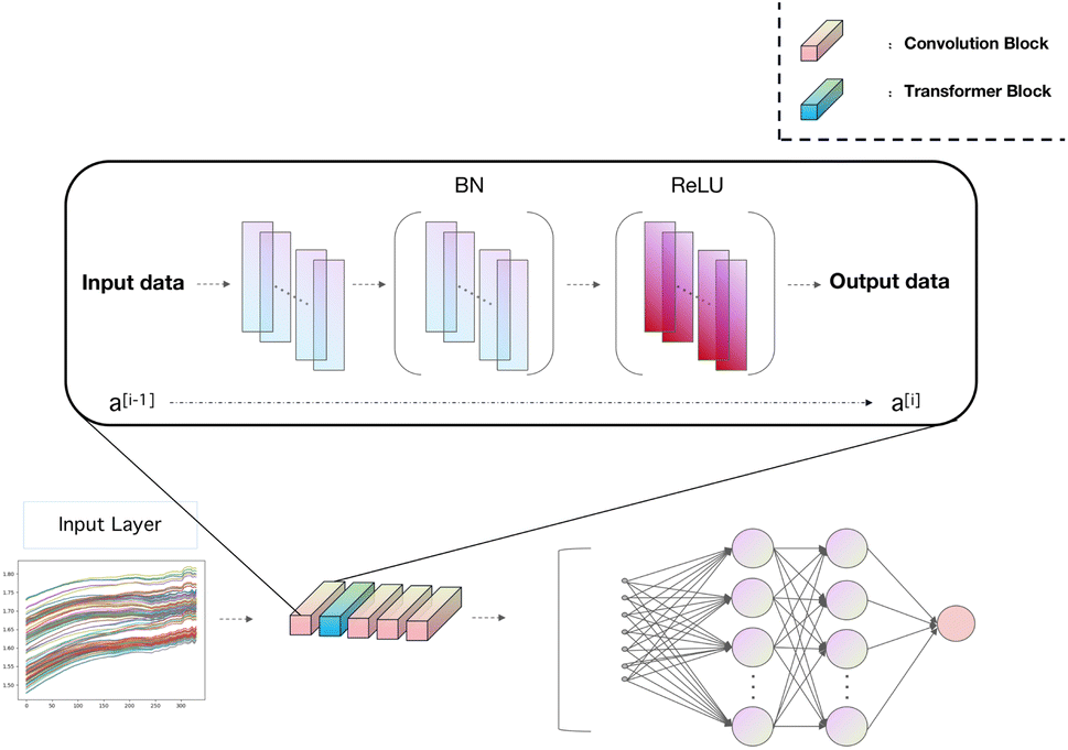 | ||
| Fig. 3 Diagram showing the structure of the spectraformer. | ||
In our model, the initial convolutional layer is configured with 16 channels, and each subsequent layer progressively doubles the channel count from its predecessor. We have standardized the stride across all convolutional layers at 2 while setting the padding value to 1 to facilitate optimal data processing. For the self-attention layer, we tested various attention heads and ultimately adopted a dual-head attention mechanism. This specific design choice aims to improve the model's ability to process and interpret complex information, thereby significantly enhancing the overall model efficacy.
After completing all feature extraction and fusion processes, all convolutional features are flattened and processed through two fully connected layers to yield classification results. The cross-entropy loss function was chosen as the primary loss function for the model to ensure superior classification results. Additionally, stochastic gradient descent (SGD) with a learning rate 0.0001 was employed to guide the gradient descent process, owing to its ease of implementation and computational efficiency. To guarantee thorough training of the model while safeguarding against overfitting, we established a training termination criterion at 200 epochs. Consequently, the training regimen will involve 200 complete cycles through the training dataset, with the process halting at this point regardless of potential performance gains. This protocol ensures uniformity and comparability in the training of the model and judiciously manages the expenditure of computational resources.
The experimental design for this study involved systematically adding or removing different components to evaluate their contributions to the model's performance and their relevance to various tasks.
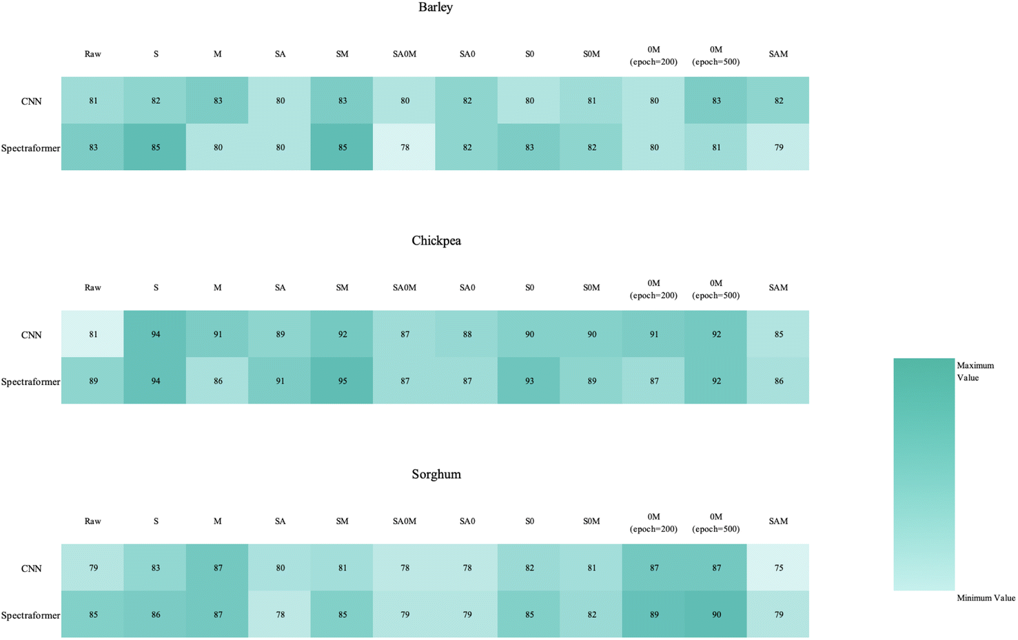 | ||
| Fig. 4 Heatmap of the overall classification accuracy for cereal variety identification using CNN and spectraformer, with different preprocessing methods (in columns) and models (in rows). | ||
In our exploration of the convolutional neural network relative to the spectraformer model, we endeavored to offset the reduction in model complexity caused by excluding the transformer module. This was attempted by integrating an extra CNN module, aiming to achieve a balance in the model's architectural intricacy.
The transformer module is instrumental in classifying near-infrared spectroscopy data and is adept at handling the spectral data's blend of global and local features.36,37 Its attention mechanism excels not only in capturing global features across the entire spectrum but also in assessing the significance of each wavelength within this global context. This dual capability allows the model to integrate a comprehensive understanding of the spectral range, enhancing classification performance significantly.
Additionally, we treat near-infrared spectroscopy data as a continuous sequence, akin to processing sentences in natural language. This approach enables our model to leverage the sequential nature of the data effectively.
Critically, the transformer's self-attention mechanism dynamically weighs each wavelength channel, recognizing varying degrees of importance across the spectrum. This process doesn't isolate channels; rather, it evaluates them within the overall spectral context, emphasizing relevant features while de-emphasizing lesser ones. This nuanced approach not only preserves the integrity of global feature comprehension but also refines it by giving weight to the most informative parts of the spectrum, thereby bolstering the model's ability to differentiate between various categories with heightened sensitivity and precision.
Furthermore, features in spectral data may exhibit long-range dependencies, such as interactions between certain wavelengths. Traditional convolutional neural networks might encounter limitations in capturing these long-range dependencies. In contrast, the transformer's self-attention mechanism excels at capturing relationships between distant features, thus elevating the modeling capability of the classification model when dealing with complex data.
As summarized in Table 1, our experimental findings confirm that placing the transformer module after the first convolutional layer yields the most favorable results. We posit several reasons behind this choice. Firstly, this configuration helps the model swiftly identify and emphasize critical features in the input data at an early stage, thereby enhancing the model's representative capacity. Secondly, it plays a pivotal role in alleviating gradient vanishing or exploding issues, thereby expediting the training convergence process.
| Model | After 1 | After 2 | After 3 |
|---|---|---|---|
| Our | 0.86 | 0.78 | 0.80 |
Moreover, spectral data often exhibit temporal and contextual dependencies. The introduction of the attention module immediately after the initial convolutional layer enables the model to incorporate contextual information earlier. This augmentation assists the model in capturing temporal and contextual relationships within the data more effectively.
Nevertheless, it is imperative to acknowledge that the optimal architecture and placement of the attention module may vary depending on the specific task and data type. Achieving the best configuration often necessitates experimentation. Additionally, different types of attention mechanisms can be explored to adapt to diverse data and tasks effectively.
Including four stacked convolutional layers, each equipped with a kernel size of 3, enables the model to extract features at various scales. Shallow layers tend to capture local details, while deeper layers are adept at encompassing more extensive contextual information. This multi-scale feature extraction enhances the model's capacity to differentiate between different categories, enriching the representation of spectral data.
Convolutional operations involve convolving input data with convolutional kernels and applying non-linear activation functions. This non-linear transformation empowers the convolutional layers to acquire abstract feature representations within spectral data, consequently elevating the model's classification performance. The progressive non-linear transformations across different layers gradually extract higher-level features.
The Rectified Linear Unit (ReLU) is widely applied in deep learning models as an effective activation function. Compared to traditional S-shaped activation functions like sigmoid or tanh, the main advantage of ReLU lies in its simplicity and mitigation of the vanishing gradient problem. The working principle of ReLU is straightforward: it passes any positive input directly and outputs zero for any negative input. This mechanism not only reduces computational complexity but also, due to its constant gradient in the positive region, helps accelerate the training process of neural networks. Additionally, ReLU introduces non-linearity, allowing the model to learn more complex representations of data. In the context of near-infrared (NIR) spectroscopy classification models, ReLU is particularly beneficial due to its ability to handle the high-dimensional and complex chemical information present in NIR data effectively. Its non-linear processing helps in capturing intricate patterns in the spectral data, which is crucial for accurate classification. Moreover, ReLU's characteristic of mitigating the gradient vanishing problem is vital in deep learning models dealing with NIR spectroscopy, where layers of the network need to learn from vast and intricate datasets.
Batch Normalization (BN) is a key technique designed to address the issue of internal covariate shifts in deep learning networks. In deep neural networks, the input distribution of intermediate layers might change due to continuous updates of layer parameters, a phenomenon known as internal covariate shift. Batch normalization addresses this issue by applying normalization processing at each layer, i.e., adjusting the mean and variance of each mini-batch of data to maintain the stability of the input distribution. This normalization process not only speeds up the training of the network but also increases the model's tolerance to initial weight settings, making the training more robust. In the case of NIR spectroscopy classification models, BN is particularly advantageous. It ensures consistent training conditions across different layers of the network, which is crucial for dealing with the variability in NIR spectral data. By stabilizing the learning process, BN allows for the use of higher learning rates, which is essential for quickly processing and analyzing the large volumes of data typical in NIR spectroscopy. This makes BN an essential component in the development of robust and efficient NIR spectroscopy classification models.
An additional advantage of convolutional operations is their ability to reduce the dimensionality of feature maps. This reduction serves a dual purpose by mitigating the number of model parameters, reducing computational costs, and addressing overfitting concerns while enhancing the model's generalization performance.
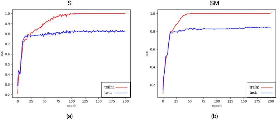
The model systematically constructs more robust feature representations by applying four layers of one-dimensional convolution with a kernel size of 3. These features can capture intricate details, patterns, and correlations within spectral data, enabling the model to classify accurately. The four layers of one-dimensional convolution with a kernel size of 3 serve as versatile components in near-infrared spectral classification. They fulfill multiple roles, encompassing local and global feature capture, multi-scale feature extraction, feature enhancement via non-linear transformations, and dimensionality reduction. These convolutional layers are indispensable for preprocessing and feature extraction in near-infrared spectral data, enriching the input information available to the classification model and enhancing classification performance (Fig. 5).
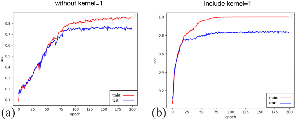 | ||
| Fig. 5 The testing accuracy curve for spectraformer with a kernel = 1 convolutional layer is (a) and the testing accuracy curve for spectraformer without a kernel = 1 convolutional layer is (b). The spectral data used is from barley, and the preprocessing method employed is the SM method. | ||
Including one-kernel convolution layers after each layer of three-kernel convolution layers allows for gradually extracting more abstract features from the original spectral data. Each convolutional layer captures information at different scales, ranging from local intricacies to global patterns. The subsequent one-kernel convolution layers further consolidate these features, enabling the model to understand better the structural nuances and relationships inherent in the spectral data.
The one-kernel convolution layers, characterized by a kernel size of 1, excel at fusing features from different channels. This fusion fosters inter-channel information interactions, enriching the holistic feature representation and elevating classifier performance.
The synergy between four layers of one-dimensional convolution with a kernel size of 3 and the subsequent one-kernel convolution layers extracts comprehensive insights from diverse perspectives within spectral data. This enables the model to comprehend spectral data's diversity and complexity better, ultimately leading to more precise classification outcomes.
In summary, combining four layers of one-dimensional convolution with a kernel size of 3, followed by one-kernel convolution layers, plays a pivotal role in feature extraction, information integration, and dimension control within near-infrared spectral classification. This amalgamation significantly enhances the model's capacity to abstractly represent spectral data, improving classification accuracy and bolstering generalization performance.
Our research offers valuable insights into spectral data analysis, thereby serving as a valuable guide for the practical application of near-infrared spectroscopy classification challenges.
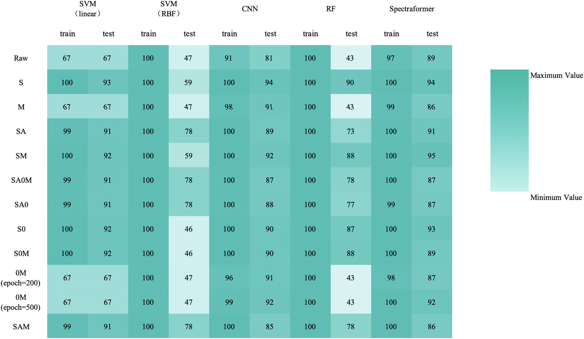
3.2 Grain species identification
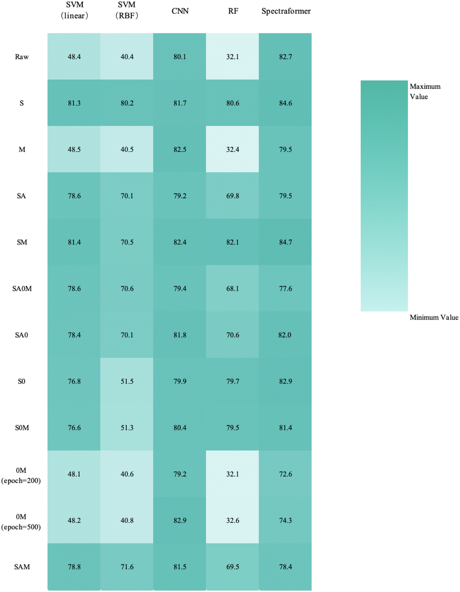
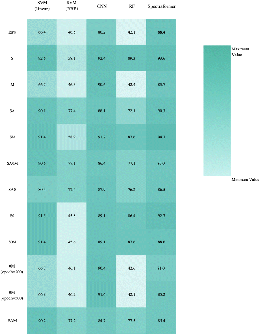
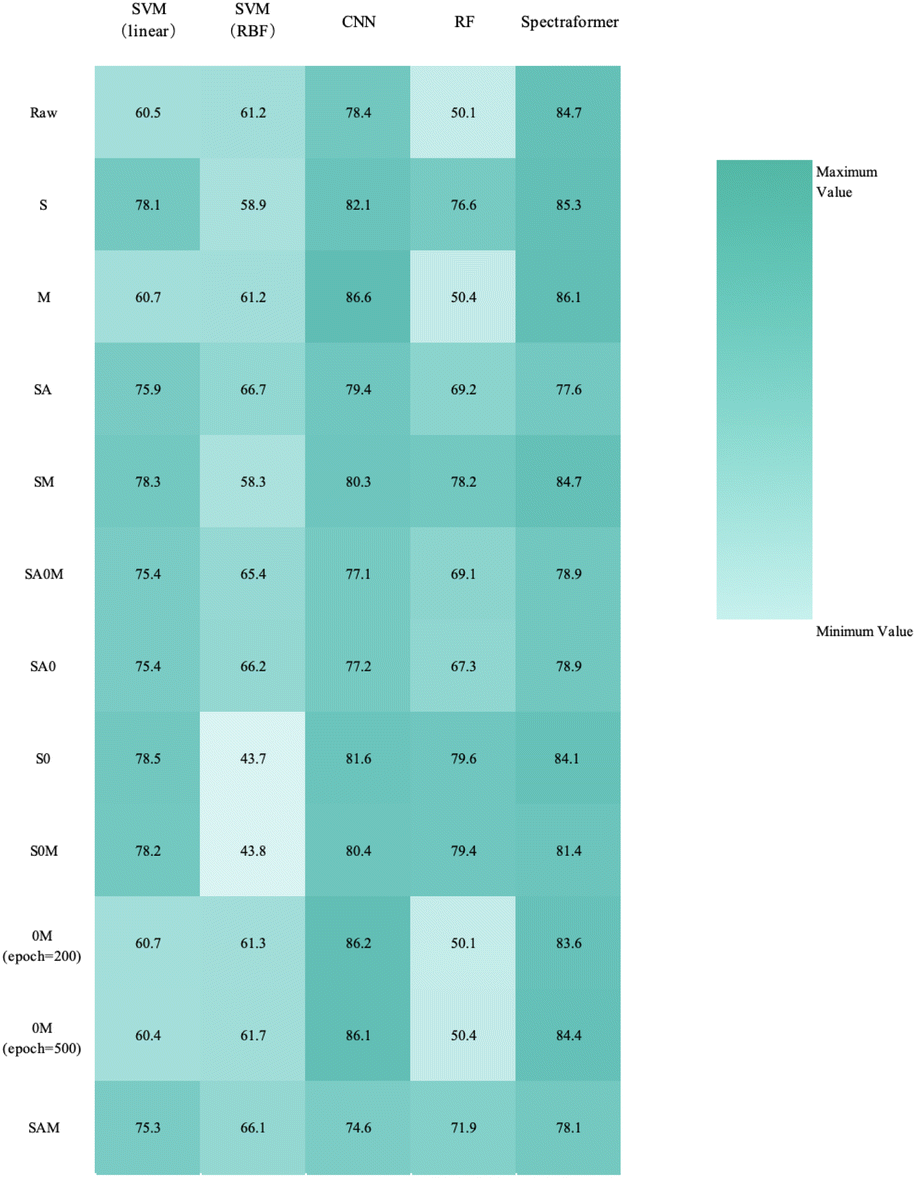
We conducted training and validation procedures involving five different algorithms on the original spectra, coupled with 10 distinct preprocessing techniques to validate these algorithms. This comprehensive evaluation involved 330 trials, with each crop type undergoing 110 assessments.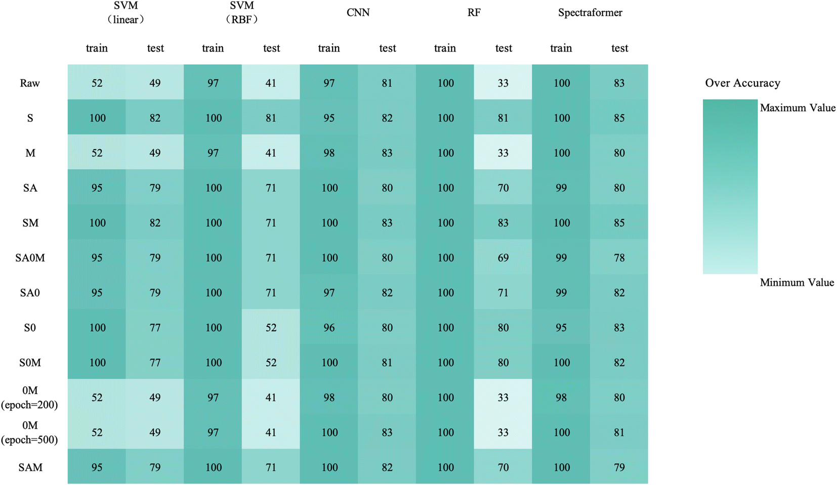 | ||
| Fig. 6 Overall classification accuracy heatmap of barley cultivar identification (N = 24 varieties and n = 1200 samples) using a combination of preprocessing methods (in rows) and models (in columns). | ||
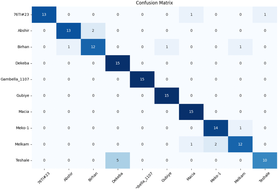
The confusion matrix in Fig. 7 displays the classification results achieved by applying data preprocessed with SM to the spectraformer model. Impressively, nine barley varieties achieved 100% correct classification, while eight varieties achieved classification accuracy surpassing the 85% mark. However, seven varieties fell short of the 80% accuracy threshold.
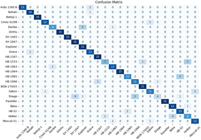 | ||
| Fig. 7 Confusion matrix of barley cultivar from the spectraformer model that achieved the best score (SM). Overall classification accuracy is 84.7%. | ||
Notably, the Deribe and Holker varieties exhibited lower classification accuracy, standing at only 60%. Deribe had a 1/3 probability of being misclassified as the Explorer variety, and Holker was nearly 1/3 likely to be classified as the Beka variety. The Shege variety experienced severe classification errors, with Shege being incorrectly classified as either the EH 1493 variety or the HB-1966 variety.
 | ||
| Fig. 8 Overall classification accuracy heatmap for chickpea cultivar identification (N = 19 varieties and n = 950 samples), using a combination of preprocessing methods (in rows) and models (in columns). | ||
Fig. 9 provides a comprehensive view through the confusion matrix for the spectraformer model applied to SM preprocessed data for classification. Notably, only one variety displayed a classification accuracy lower than 80%, with the Ejere variety potentially being misclassified as either the Habru or Shasho variety. Impressively, twelve varieties achieved perfect accuracy in classification.
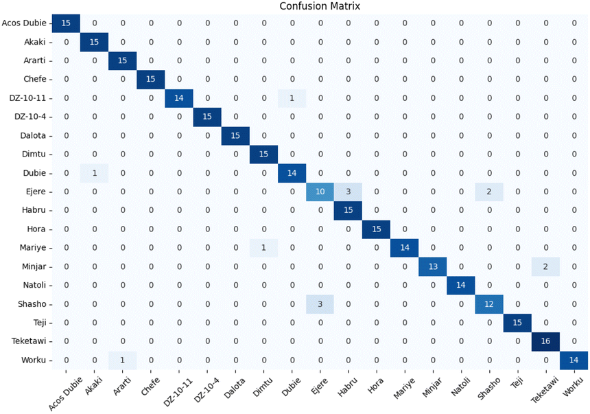 | ||
| Fig. 9 Confusion matrix of chickpea cultivar from the spectraformer model that achieved the best score (SM). Overall classification accuracy is 95.4%. | ||
 | ||
| Fig. 10 Overall classification accuracy heatmap for sorghum cultivar identification (N = 10 varieties and n = 500 samples), using a combination of preprocessing methods (in rows) and models (in columns). | ||
 | ||
| Fig. 11 The testing accuracy curve obtained with raw data is represented as (a), the testing accuracy curve obtained with preprocessed data using method M is represented as (b), the testing accuracy curve with preprocessed data using method 0M and epoch = 200 is represented as (c), and the testing accuracy curve with preprocessed data using method 0M and epoch = 500 is represented as (d). | ||
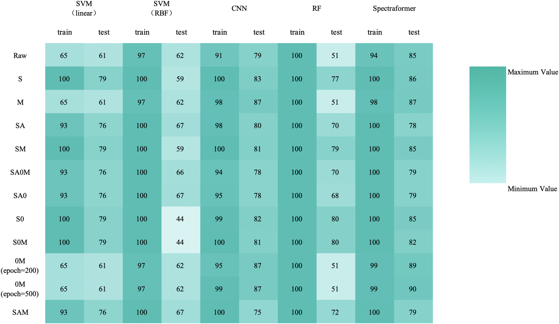
While data preprocessed with the 0M and M methods, as well as raw data input into the spectraformer model, exhibited the highest testing accuracy, their testing accuracy curves were observed to be less stable, as depicted in Fig. 11(a)–(c). Conversely, data preprocessed with the S and SM methods, although slightly lower by 1–2 percentage points, displayed stable accuracy curves, as evidenced in Fig. 13(a) and (b). It's worth noting that while fluctuating curves may yield better results in specific cases, predicting such scenarios can be challenging. Smooth curves are generally more interpretable and comprehensible, signifying stable model training less susceptible to randomness. This enhances the model's reliability and ensures more consistent performance across diverse datasets and experimental conditions.
Fig. 12 illustrates the confusion matrix for 0M (epoch = 200) preprocessing. Among the ten varieties, four achieved perfect classification accuracy, with only the Teshale variety falling below the 80% threshold, having a 1/3 probability of being misclassified as Dekeba.
 | ||
| Fig. 12 Confusion matrix of sorghum cultivar from the spectraformer model that achieved score (0M, epoch = 200). Overall classification accuracy is 89.3%. | ||
 | ||
| Fig. 13 The testing accuracy curve obtained with preprocessed data using method S is represented as (a), and the testing accuracy curve obtained with preprocessed data using method SM is represented as (b). | ||
In this study, a range of k-fold cross-validation methods, from 2-fold to 10-fold, were meticulously tested. It was conclusively determined that 5-fold cross-validation yielded the most optimal performance in this experimental context. This decision was informed by a holistic consideration of factors, including model stability, accuracy, and computational efficiency.
Upon reviewing Fig. 14, 15, and 16, it was observed that the spectraformer model consistently demonstrated high accuracy across both 5-fold cross-validation and the conventional 7:3 data split when employing both S and SM preprocessing methods. Delving into specifics, the SM preprocessing method exhibited superior performance in the barley dataset during 5-fold cross-validation, achieving an impressive average accuracy rate of 84.7%. Similarly, this method attained the highest average accuracy of 94.7% with the chickpea dataset. In the case of the sorghum dataset, the SM method again proved to be the most effective, reaching an average accuracy rate of 84.7%. These findings underscore the adaptability and efficiency of the SM preprocessing method across diverse datasets.
 | ||
| Fig. 14 Overall classification 5-fold cross-validation accuracy heatmap for barley cultivar identification (N = 24 varieties and n = 1200 samples), using a combination of preprocessing methods (in rows) and models (in columns). | ||
 | ||
| Fig. 15 Overall classification 5-fold cross-validation accuracy heatmap for barley cultivar identification (N = 24 varieties and n = 1200 samples), using a combination of preprocessing methods (in rows) and models (in columns). | ||
 | ||
| Fig. 16 Overall classification 5-fold cross-validation accuracy heatmap for barley cultivar identification (N = 24 varieties and n = 1200 samples), using a combination of preprocessing methods (in rows) and models (in columns). | ||
By comparing the outcomes of the 5-fold cross-validation with the results from splitting the dataset into a validation set using a 7:3 ratio, we can observe a notable reduction in accuracy when employing the 5-fold cross-validation in conjunction with the 0M preprocessing condition. This suggests that the 0M preprocessing method might compromise the spectraformer model's performance stability, thereby rendering it less suitable as a universal preprocessing approach.
The collective correct classification accuracy for the 24 barley varieties, 19 chickpea varieties, and 10 sorghum varieties reached 85%, 95%, and 86%, respectively. It is worth noting that prior research has similarly indicated that while not all categories may achieve perfect classification, near-infrared spectra retain the potential for robust variety identification.
The extensive experiments conducted with barley, chickpea, and sorghum data show that deep learning models consistently exhibit superior robustness compared to traditional machine learning approaches. Deep learning models consistently achieve accuracies of nearly 80% or even higher across various preprocessing methods, underscoring their adaptability and capacity to capture complex patterns.
It is noteworthy that traditional machine learning models rely more on the relationships within the data. Models employing SVM (linear) and Random Forest generally outperform those using SVM (RBF), implying a clear linear correlation within the spectral data. The relatively high accuracy of the SVM (linear) model suggests that the spectral data exhibits linear separability within the feature space, enabling linear classifiers to distinguish spectral data from different categories effectively. In contrast, SVM (RBF) may be more prone to overfitting when mapping the data to a higher-dimensional feature space, potentially leading to reduced model performance.
Conversely, the high accuracy achieved by the Random Forest model may indicate the presence of intricate yet linearly separable patterns in the spectral data. Random Forest, an ensemble learning method, excels at capturing non-linear data relationships by combining the outcomes of multiple decision trees while benefiting from the data's underlying linear structure.
It's essential to note that while the accuracy of traditional machine learning models remains consistent when classifying the three types of data (original, preprocessed with M, and preprocessed with 0M), this does not imply that M and 0M preprocessing had no impact on the data. In the realm of deep learning, training on the original data yields test accuracy curves with more fluctuations compared to training on data preprocessed with M or 0M, as evidenced in Fig. 11(a)–(c). This phenomenon could be attributed to the potential loss or amplification of information in specific features resulting from the M and 0M preprocessing, as deep learning models are sensitive to the scale and distribution of data. Such sensitivity can lead to increased fluctuations in test accuracy curves.
In contrast, traditional machine learning models, particularly linear and tree-based models, tend to be less sensitive to the absolute scale of features. These models emphasize relative relationships and patterns between features, exhibiting minimal concern for the absolute numerical values of features. Consequently, in traditional machine learning, the loss or amplification of information induced by normalization has a relatively insignificant impact on model performance.
Indeed, deep learning models have demonstrated remarkable adaptability, rendering the nature of data relationships less limiting. Deep learning exhibits the capability to learn suitable feature representations for data, irrespective of whether the data exhibits linear or non-linear relationships, resulting in exceptional accuracy. The strength of deep learning models lies in their multi-layered neural network architectures, which inherently possess the capacity to automatically unearth and express intricate patterns and correlations within the data. Furthermore, deep learning models excel in processing high-dimensional data, extracting valuable information from various input features. This attribute proves particularly advantageous for complex data types such as spectral data.
Deep learning models are typically trained using the backpropagation algorithm, which autonomously fine-tunes the model's weights and parameters to minimize the loss function, enhancing the model's alignment with the data. This adaptability empowers deep learning models to consistently achieve outstanding performance across diverse data relationship scenarios encompassing linear, non-linear, and highly intricate data patterns.
While non-linear discriminative models like SVM possess unique capabilities for handling small datasets and can harness spectral information to achieve accuracy levels approaching those of deep learning models, this underscores the importance of spectral information, particularly in the context of barley variety identification. However, it is essential to recognize that deep learning models also offer advantages in addressing non-linearity and handling large datasets, rendering them an ideal choice for barley variety identification. Consequently, the selection of the appropriate model algorithm should be guided by considerations such as dataset size and the inherent nature of the data.
4 Conclusions
In this comprehensive study, we harnessed the power of near-infrared hyperspectral imaging in conjunction with deep learning to effectively categorize various crops. Our dataset encompassed a substantial volume, featuring 1200 barley grains, 950 chickpeas, and 500 sorghum grains, facilitating a rigorous analysis.The results obtained in our research underscore the exceptional performance of the transformer module in the domain of near-infrared spectroscopy. While CNNs may occasionally achieve similar accuracy levels, it is vital to clarify that this does not inherently imply superiority over our proposed model. Transformers, particularly when operating on larger datasets, consistently exhibit superior performance, showcasing their robustness and formidable generalization capabilities.
Moreover, our multi-model comparative experiments unequivocally demonstrate that our proposed model consistently outperforms other models across various performance metrics, with accuracy being a prominent factor.
Furthermore, our experiments have unveiled the profound impact of different preprocessing methods on spectral data. These findings provide substantial empirical evidence supporting the utility of small-scale near-infrared spectrometers and machine-learning techniques for precisely identifying crop varieties.
In summary, this study not only leverages state-of-the-art technology and methodologies but also underscores the remarkable potential of combining near-infrared hyperspectral imaging with deep learning, offering valuable insights into the domain of crop variety identification.
Conflicts of interest
There are no conflicts to declare.Acknowledgements
This work is supported by the National Key R&D Plan under Grant No. 2021YFF0601200 and 2021YFF0601204.Notes and references
- M. B. Priyadarshi, A. Sharma, K. Chaturvedi, R. Bhardwaj, S. Lal, M. Farooqi, S. Kumar, D. Mishra and M. Singh, Legume Res., 2023, 46, 251–256 Search PubMed.
- I. Ejaz, S. He, W. Li, N. Hu, C. Tang, S. Li, M. Li, B. Diallo, G. Xie and K. Yu, Front. Plant Sci., 2021, 12, 720022 CrossRef PubMed.
- M. Blanco and I. Villarroya, TrAC, Trends Anal. Chem., 2002, 21, 240–250 CrossRef CAS.
- J. S. Shenk, J. J. Workman Jr and M. O. Westerhaus, Handbook of near-infrared analysis, CRC Press, 2007, pp. 365–404 Search PubMed.
- J. U. Porep, D. R. Kammerer and R. Carle, Trends Food Sci. Technol., 2015, 46, 211–230 CrossRef CAS.
- A. Munawar, Y. Yunus, D. Devianti and P. Satriyo, IOP Conf. Ser. Earth Environ. Sci., 2021, 012036 CrossRef.
- B. K. Wilson, H. Kaur, E. L. Allan, A. Lozama and D. Bell, Am. J. Trop. Med. Hyg., 2017, 96, 1117 CAS.
- R. Giovanni, Smartphone-Based Food Diagnostic Technologies: A Review, Sensors, 2017, 17(6), 1453 CrossRef PubMed.
- Y. LeCun, L. Bottou, Y. Bengio and P. Haffner, Proc. IEEE, 1998, 86, 2278–2324 CrossRef.
- J. Yang, J. Wang, G. Lu, S. Fei, T. Yan, C. Zhang, X. Lu, Z. Yu, W. Li and X. Tang, Comput. Electron. Agric., 2021, 190, 106431 CrossRef.
- D. Rong, H. Wang, Y. Ying, Z. Zhang and Y. Zhang, Comput. Electron. Agric., 2020, 175, 105553 CrossRef.
- J. Acquarelli, T. van Laarhoven, J. Gerretzen, T. N. Tran, L. M. Buydens and E. Marchiori, Anal. Chim. Acta, 2017, 954, 22–31 CrossRef CAS PubMed.
- X. Zhang, T. Lin, J. Xu, X. Luo and Y. Ying, Anal. Chim. Acta, 2019, 1058, 48–57 CrossRef CAS PubMed.
- L. Ling-qiao, P. Xi-peng, F. Yan-chun, Y. Li-hui, H. Chang-qin and Y. Hui-hua, Spectrosc. Spectral Anal., 2019, 39, 3606–3613 Search PubMed.
- X. Zhang, J. Yang, T. Lin and Y. Ying, Trends Food Sci. Technol., 2021, 112, 431–441 CrossRef CAS.
- C. Cui and T. Fearn, Chemom. Intell. Lab. Syst., 2018, 182, 9–20 CrossRef CAS.
- P. Fu, Y. Wen, Y. Zhang, L. Li, Y. Feng, L. Yin and H. Yang, J. Innovative Opt. Health Sci., 2022, 15, 2250021 CrossRef CAS.
- A. Vaswani, N. Shazeer, N. Parmar, J. Uszkoreit, L. Jones, A. N. Gomez, Ł. Kaiser and I. Polosukhin, Advances in neural information processing systems, 2017, vol. 30 Search PubMed.
- K. Ahmed, N. S. Keskar and R. Socher, arXiv, 2017, preprint, arXiv:1711.02132 Search PubMed.
- K. Xu, J. Ba, R. Kiros, K. Cho, A. Courville, R. Salakhudinov, R. Zemel and Y. Bengio, International conference on machine learning, 2015, pp. 2048–2057 Search PubMed.
- M.-T. Luong, H. Pham and C. D. Manning, arXiv, 2015, preprint, arXiv:1508.04025, DOI:10.48550/arXiv.1508.04025.
- D. Bahdanau, K. Cho and Y. Bengio, arXiv, 2014, preprint, arXiv:1409.0473, DOI:10.48550/arXiv.1409.0473.
- F. Kosmowski and T. Worku, PloS One, 2018, 13, e0193620 CrossRef PubMed.
- L. Hao-xiang, Z. Jing, L. Ling-qiao, L. Zhen-bing, Y. Hui-hua, F. Yan-chun and Y. Li-hui, Spectrosc. Spectral Anal., 2021, 41, 1782–1788 Search PubMed.
- X. Miao, Y. Miao, H. Gong, S. Tao, Z. Chen, J. Wang, Y. Chen and Y. Chen, Spectrochim. Acta, Part A, 2021, 257, 119700 CrossRef CAS PubMed.
- P. Mishra, J. M. Roger, F. Marini, A. Biancolillo and D. N. Rutledge, Chemom. Intell. Lab. Syst., 2021, 212, 104190 CrossRef CAS.
- C. Cortes and V. Vapnik, Mach. Learn., 1995, 20, 273–297 Search PubMed.
- L. Breiman, Mach. Learn., 2001, 45, 5–32 CrossRef.
- S. Khan, M. Naseer, M. Hayat, S. W. Zamir, F. S. Khan and M. Shah, ACM Comput. Surv., 2022, 54, 1–41 CrossRef.
- J. Wang, C.-Y. Hsieh, M. Wang, X. Wang, Z. Wu, D. Jiang, B. Liao, X. Zhang, B. Yang and Q. He, et al., Nat. Mach. Intell., 2021, 3, 914–922 CrossRef.
- V. Venkatasubramanian and V. Mann, Curr. Opin. Chem. Eng., 2022, 36, 100749 CrossRef.
- O. Devos, C. Ruckebusch, A. Durand, L. Duponchel and J.-P. Huvenne, Chemom. Intell. Lab. Syst., 2009, 96, 27–33 CrossRef CAS.
- V. G. K. Cardoso and R. J. Poppi, Microchem. J., 2021, 164, 106052 CrossRef CAS.
- M. Li, F. Chen, M. Lei and C. Li, Guangpuxue Yu Guangpu Fenxi, 2016, 36, 2793–2797 CAS.
- H. Qiao, X. Shi, H. Chen, J. Lyu and S. Hong, Soil Tillage Res., 2022, 215, 105223 CrossRef.
- S. d'Ascoli, H. Touvron, M. L. Leavitt, A. S. Morcos, G. Biroli and L. Sagun, International Conference on Machine Learning, 2021, pp. 2286–2296 Search PubMed.
- Z. Dai, H. Liu, Q. V. Le and M. Tan, Advances in neural information processing systems, 2021, vol. 34, pp. 3965–3977 Search PubMed.
Footnote |
| † https://github.com/zzd119/cz-data |
| This journal is © The Royal Society of Chemistry 2024 |