
 Open Access Article
 This Open Access Article is licensed under a Creative Commons Attribution-Non Commercial 3.0 Unported Licence
Carbon Kagome nanotubes—quasi-one-dimensional nanostructures with flat bands†
Husan Ming Yu‡
 a,
Shivam Sharma‡b,
Shivang Agarwalc,
Olivia Liebmana and
Amartya S. Banerjee*a
a,
Shivam Sharma‡b,
Shivang Agarwalc,
Olivia Liebmana and
Amartya S. Banerjee*a
aDepartment of Materials Science and Engineering, University of California, Los Angeles, CA 90095, USA. E-mail: asbanerjee@ucla.edu; Tel: +1-763-656-7830
bDepartment of Aerospace Engineering and Mechanics, University of Minnesota, Minneapolis, MN 55455, USA
cDepartment of Electrical and Computer Engineering, University of California, Los Angeles, CA 90095, USA
First published on 5th January 2024
Abstract
In recent years, a number of bulk materials and heterostructures have been explored due their connections with exotic materials phenomena emanating from flat band physics and strong electronic correlation. The possibility of realizing such fascinating material properties in simple realistic nanostructures is particularly exciting, especially as the investigation of exotic states of electronic matter in wire-like geometries is relatively unexplored in the literature. Motivated by these considerations, we introduce in this work carbon Kagome nanotubes (CKNTs)—a new allotrope of carbon formed by rolling up Kagome graphene, and investigate this material using specialized first principles calculations. We identify two principal varieties of CKNTs—armchair and zigzag, and find both varieties to be stable at room temperature, based on ab initio molecular dynamics simulations. CKNTs are metallic and feature dispersionless states (i.e., flat bands) near the Fermi level throughout their Brillouin zone, along with an associated singular peak in the electronic density of states. We calculate the mechanical and electronic response of CKNTs to torsional and axial strains, and show that CKNTs appear to be more mechanically compliant than conventional carbon nanotubes (CNTs). Additionally, we find that the electronic properties of CKNTs undergo significant electronic transitions—with emergent partial flat bands and tilted Dirac points—when twisted. We develop a relatively simple tight-binding model that can explain many of these electronic features. We also discuss possible routes for the synthesis of CKNTs. Overall, CKNTs appear to be unique and striking examples of realistic elemental quasi-one-dimensional materials that may display fascinating material properties due to strong electronic correlation. Distorted CKNTs may provide an interesting nanomaterial platform where flat band physics and chirality induced anomalous transport effects may be studied together.
1 Introduction
Over the past two decades, the design, discovery and characterization of nanomaterials and nanostructures with special features in their electronic band structure has gained prominence. Exemplified famously by the case of linear dispersive relations in graphene (associated with massless Dirac fermions1,2), such features often point to the existence of exotic electronic states, and the possibility of realizing unconventional electromagnetic, transport and optical properties in real systems. In recent years, materials and structures featuring dispersionless electronic states or flat bands have been heavily investigated due to the fact that electrons associated with such states have quenched kinetic energies§ (are spatially localized), and interact in the strong correlation regime.3–6 This manner of interaction leads to a variety of fascinating materials phenomena, including superconductivity,3,7 ferromagnetism,8 Wigner crystallization,9,10 and the fractional quantum Hall effect.11–14Along these lines, moiré superlattices in twisted bilayers8,15–19 and materials with tailored atomic lattices20–23 have received much attention since they feature flat bands and rich electron physics. In order to observe and maintain desirable electronic properties, such systems usually involve some degree of engineering, and more often, a fine control over important system parameters (e.g. bilayer twists at specific magic angles,24 or a critical magnetic field strength in quasi-two-dimensional (2D) network structures25,26). Therefore, a strand of recent investigations has focused on the synthesis and characterization of materials which feature electronic flat bands due to their natural atomic arrangements.27–35 Exotic electronic states hosted by such materials can be stable with respect to perturbations such as changes in temperature or applied strains, and they can often display such states without external fields—features which make them suitable for device applications. Alongside these experimental studies, computational investigations have also probed elemental versions of such materials, i.e., stable bulk or 2D nanomaterials made of a single species of atom that can feature unusual electronic states by virtue of their atomic arrangements alone.36–41 The present study extends this particular line of work to the important case of quasi-one-dimensional (1D) nanomaterials featuring flat bands, which have generally received far less attention in the literature.¶
The possibility of realizing flat band physics and exotic states of electronic matter in wire-like geometries is particularly exciting. While well known theoretical considerations45,46 appear to preclude the existence of long range order in low dimensional systems (necessary, e.g. in realizing superconducting states), such restrictions do not necessarily apply to the quasi-one-dimensional structures considered here.47 In fact, there are reasons to expect that the screw transformation symmetries and quantum confinement effects often associated with such systems can actually result in enhancement of collective or correlated electronic properties,48–50 and that such properties are likely to be manifested in manners that are quite different from bulk phase materials. In particular, materials such as the ones considered in this work can be chiral—due to intrinsic or applied twists—and therefore, feature anomalous transport (the Chiral Induced Spin Selectivity, or CISS effect51,52). The exploration of simultaneous manifestations of such effects along with correlated electron physics has begun fairly recently.53–56 We posit that the carbon nanostructures explored here are likely to emerge as a possible material platform for such studies in the future.
Due to its unique allotrope forming features and versatility,57–59 carbon is particularly attractive as a building block of novel materials. A large number of computational studies have recently been devoted to 2D and bulk allotropes of carbon displaying Dirac cones, flat bands and non-trivial topological states.37,60–67 On the other hand, although several 1D allotropes of carbon are well known,68–79 none of these systems are usually associated with flat band physics. As far as we can tell, there have been only a few earlier attempts at producing and investigating flat bands in realistic 1D nanomaterials of carbon: partially flat bands in zigzag graphene nanoribbons,80 spin polarized flat bands in hydrogenated carbon nanotubes,81 and moiré type flat bands in chiral carbon nanotubes with collapsed structures82,83 or incommensurate double wall geometries.84 Our contribution aims to address this particular gap in the literature by studying a family of realistic 1D carbon nanostructures that naturally feature flat bands throughout their Brillouin zone. The flat bands in the structures presented here arise out of geometric and orbital frustration and without the aid of dopant or major structural instability effects, as employed in the aforementioned studies. Moreover, as we demonstrate, these dispersionless electronic states show fascinating transitions as the structures are subjected to strains, while also proving to be robust and retaining many desirable characteristics in some respects.
To obtain a 1D carbon nanostructure with flat bands, our starting point is a planar sheet of Kagome graphene. We then “roll up” this 2D material along different directions to obtain Carbon Kagome Nanotubes (CKNTs). Kagome graphene and related bulk structures have recently received much attention in the materials literature,36,38–41,85,86 and also in the physics literature, where the material is often identified as a “decorated honeycomb” or “star lattice” structure.23,87–92 Although Kagome graphene remains to be experimentally synthesized, successful synthesis of a variant of this material, i.e., nitrogen-doped graphene on a silver substrate—a 2D material with a Kagome pattern, has been carried out recently.93,94 Moreover, synthesis of novel complex nanotube structures in general (see e.g. ref. 95) and through the roll-up of 2D sheets in particular, is fairly common (see e.g. ref. 96), thus suggesting that CKNTs can be synthesized in the near future.
In this work, we introduce CKNTs, and carry out a thorough and systematic first principles characterization of this material in terms of its structural, mechanical and electromechanical properties. Wherever relevant, we provide comparisons of the properties of CKNTs against those of conventional carbon nanotubes (CNTs). All CKNTs studied here are metallic and feature flat bands (throughout their Brillouin zone) near the Fermi level, along with an associated singular peak in the electronic density of states. We show in particular that CKNTs appear to be more mechanically compliant when compared against CNTs, and that their electronic properties undergo significant electronic transitions—with emergent partial flat bands and Dirac points—when subjected to torsional strains. Our studies are made possible largely due to a suite of recently developed symmetry adapted electronic structure calculation techniques,97–103 that allow ab initio calculations of 1D materials and their deformed states to be carried out accurately and efficiently. We also develop a π-electron based tight binding model that includes up to next–nearest–neighbor interactions, which is able to capture many of the electronic properties of CKNTs, as revealed via first principles data.
The rest of the paper is organized as follows: Section 2 describes the geometry of the materials under study (subsection 2.1), as well as various aspects of the specialized first principles computational techniques used in this work (subsection 2.2). Section 3 presents results, touching on structural (subsection 3.1), mechanical (subsection 3.2), electronic (subsection 3.3.1) and electromechanical (subsection 3.3.2) aspects. We discuss possible routes to the synthesis of CKNTs in subection 3.4 and conclude in Section 4. Details of the tight binding model for CKNTs are presented in Appendix A.
2 Material and methods
In this section, we introduce the geometry of carbon Kagome nanotubes (CKNTs) and their construction from Kagome graphene through the “roll up” procedure commonly employed in other similar types of nanomaterials.104,105 We also provide an outline of the various computational and theoretical methods used in our study.2.1 From Kagome graphene to carbon Kagome nanotubes
Several recent studies have explored the structure of Kagome graphene sheets and related bulk structures.23,36,38,39,41,85 As a starting point, we first consider the geometry of Kagome graphene. The hexagonal unit cell of this 2D material consists of 6 carbon atoms that form a pair of equilateral triangles, as shown in Fig. 1. We used the planewave code ABINIT106–108 to optimize the geometry of this structure. Our calculations employed norm conserving Troullier–Martins pseudopotentials,109 an energy cutoff of 50 Ha, 21 × 21 × 1 k-point sampling and Fermi–Dirac smearing of 0.001 Ha. These parameters were sufficient to produce accurate energies, forces and cell stresses for the pseudopotentials chosen.99 We employed both Perdew–Wang110 local density approximation (LDA) and Perdew–Burke–Ernzerhof (PBE)111 generalized gradient approximation (GGA) exchange correlation functionals. At the end of the relaxation procedure, the atomic forces were typically of the order of 10−5 Ha bohr−1, while the cell stresses were of the order of 10−8 Ha bohr−3.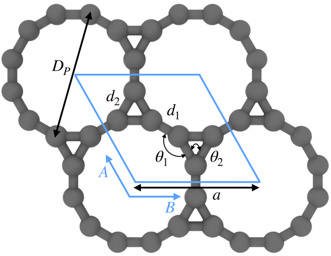 | ||
| Fig. 1 Unit cell of Kagome graphene with various structural parameters indicated. The angle θ1 is 150°, while θ2 is 60°. The other parameters can be found in Table 1. | ||
Table 1 shows that the optimized structural parameters obtained by us are in very good agreement with the literature. As expected,112 the LDA bond lengths are somewhat shorter than those obtained through functionals involving gradient corrections, although the variations observed are quite minor overall. Notably, the intertriangle C–C bond length was found to be slightly smaller than the bond length corresponding to the triangle sides. Additionally, the calculated bond angles were found to be 60° (in-triangle) and 150° (inter-triangle) almost perfectly, consistent with the literature. Next, following the construction of carbon nanotubes from graphene,104,113,114 we rolled up the optimized flat Kagome graphene structures into seamless cylinders and arrived at carbon Kagome nanotubes (see Fig. 2). Depending on the direction of rolling, the tubes maybe armchair, zigzag or chiral, with non-negative integers (n, m) denoting the chirality indices. In this work, we focus exclusively on armchair (i.e., (n, n)) and zigzag (i.e., (n, 0)) nanotubes (illustrated in Fig. 3). The index n for such achiral tubes indicates the degree of cyclic symmetry about the tube axis. An investigation of chiral CKNTs is the scope of future work. Notably, the replacement of hexagons in conventional CNTs, by dodecagonal rings in CKNTs, results in a structure with more porous sidewalls, and suggests the use of this material in filtration,115 desalination116 and electrochemical storage applications.117–119
| Parameters | Current work | Literature |
|---|---|---|
| a (Å) | 5.1370a(5.1662)b | 5.2085c, 5.2087d, 4.46e |
| d1 (Å) | 1.3402a(1.3400)b | 1.3559c, 1.3567d, 1.50e |
| d2 (Å) | 1.4078a(1.4206)b | 1.4305c, 1.4299d, 1.53e |
| Dp (Å) | 5.3090a(5.3331)b | 5.3817c, 5.3829d |
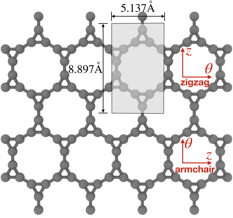 | ||
| Fig. 2 Roll-up construction of CKNTs, starting from a sheet of Kagome graphene. θ denotes the direction of roll up, while z denotes the tube axis direction. The 12 atoms shown in the shaded region are the representative atoms in the fundamental domain used for Helical DFT98,99 calculations. The domain size parameters illustrated above correspond to calculations based on LDA exchange-correlation. | ||
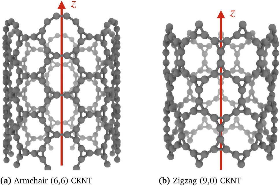 | ||
| Fig. 3 Two varieties of CKNTs investigated in this work: (a) Armchair (n, n) and (b) zigzag (n, 0) tubes. The tube radii are 0.85 nm and 0.74 nm, respectively for the above examples. n is the cyclic symmetry group order about the tube axis. | ||
2.2 Computational methods
We outline the computational methods employed in this work to study CKNTs. These include specialized, real-space symmetry adapted first principles simulations (using the Helical DFT code98,99) and periodic plane-wave calculations (based on the ABINIT,106–108 Quantum Espresso120–122 and PWDFT123–126 codes), to augment the Helical DFT results. A tight-binding model which is able to replicate many of the electronic properties revealed by the above first principles calculations is detailed separately in A. In what follows, the atomic unit system with is used throughout, unless mentioned otherwise. We will denote the standard orthonormal basis of with eX, eY, eZ. Lowercase boldface letters will denote vectors in three dimensions, while uppercase boldface will denote matrices.
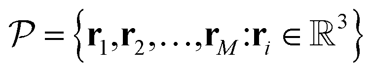 are the coordinates of the representative atoms in the simulation cell (or fundamental domain), then the collection of coordinates of the entire structure can be expressed as:
 | (1) |
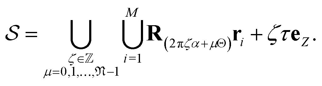
Thus, the symmetry group of the nanotube consists of the collection of isometries (i.e., rotations and translations):
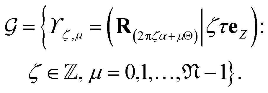 | (2) |
 is a natural number that captures cyclic symmetries in the nanotube, with the angle
 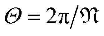 (i.e.,
  is the same as n in armchair (n, n) and zigzag (n, 0) nanotubes). The scalar α is related to the applied or intrinsic twist in the structure, with the amount of twist per unit length measured as β = 2πα/τ. The parameter τ is related to the pitch of screw transformation symmetries in the nanotube, and variations in this quantity enable extensions and compressions about the tube axis to be captured.
For the CKNTs considered in this work, we have employed an orthogonal unit cell with 12 representative atoms, as shown in Fig. 2. The parameter α takes values between 0 and 1, with α = 0 representing untwisted structures. The value of τ as suggested by the roll-up construction105,129 is 5.137 Å and 8.897 Å for undeformed armchair and zigzag CKNTs, respectively.
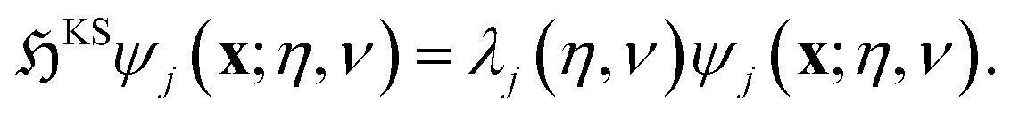
Helical DFT uses a higher order finite difference discretization scheme in helical coordinates97,98 to solve the following symmetry adapted equations of Kohn–Sham DFT over the fundamental domain:
 | (3) |
The Kohn–Sham Hamiltonian operator:
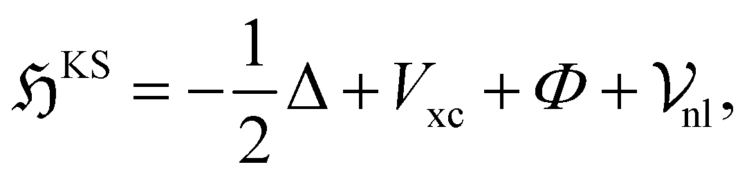 | (4) |
consists of kinetic energy, exchange correlation, electrostatic contribution (i.e., both electron–electron and electron–nucleus interactions) and non-local psudopotential130 terms. The symmetry-adapted quantum numbers  , and serve to label the eigenstates and electronic occupation numbers of the system (analogous to ‘k-points’ in periodic calculations of solids), along helical and cyclic symmetry directions, respectively. At the end of self-consistent solution of the above equations, the system's ground state electronic free energy per unit fundamental domain may be calculated. We will denote this quantity as
  to signify its explicit dependence on the positions of the representative atoms within the fundamental domain
  , the fundamental domain itself
  , and the symmetry group of the structure under consideration
  . By introducing variations in
  and by minimizing
  with respect to the coordinates of the representative atoms, Helical DFT can be employed for ab initio exploration of the deformation response of a nanomaterial under torsional or axial loads.99
In order to facilitate the large number of ground state electronic structure calculations of various CKNTs as well as their electromechanical response under applied deformations, Helical DFT simulations were carried out in three stages. First, for a given nanotube and applied strain parameters, ab initio structural relaxation calculations were carried out using a mesh spacing of h = 0.3 bohr, and by sampling 15 reciprocal space points in the η direction. These discretization choices are sufficient to produce chemically accurate forces and ground state energies for the norm conserving pseudopotential130,131 used to model the carbon atoms in this work.99 Atomic relaxation was carried using the Fast Inertial Relaxation Engine132 and calculations were continued until each atomic force component on every atom in the simulation cell reached 0.001 Ha bohr−1 or lower. Next, for each relaxed structure, we redid a self-consistent calculation using the finest discretization parameters that could be reliably employed within computational resource constraints. This corresponds to a mesh spacing of h = 0.25 bohr and 21 reciprocal space points in the η direction. This calculation step enables accurate calculations of energetics and stiffness parameters to be carried out.99 Finally, using the self consistent densities and potentials obtained through the above step, we performed a single Hamiltonian diagonalization step using 45 reciprocal space points in the η direction. The eigenstates so obtained were used for band diagram and electronic density of states calculations that are presented in Section 3.
For all Helical DFT calculations, we used the Perdew–Wang parametrization133 of the LDA.127 We did not observe any major qualitative differences in the electronic properties between the LDA results presented here and those produced using gradient corrected functionals.111 We also employed 12th order finite differences,98,100,134–139 vacuum padding of 10 bohr in the radial direction and 1 milli-Hartree of smearing using the Fermi–Dirac distribution. The pseudopotential employed was generated using the Troullier–Martins scheme,109,131 and is identical to the one used for the flat sheet calculations presented earlier (Section 2.1).
2.3 Plane-wave DFT calculations
We used plane-wave DFT140,141 for carrying out a few additional first principles calculations of CKNTs. Specifically, we investigated the dynamic stability of undistorted CKNTs by performing ab inito molecular dynamics (AIMD) simulations. The highly scalable PWDFT code123–126 was used for this purpose. We investigated two generic CKNTs—one each of the zigzag and armchair varieties—with radii of 0.75 and 0.85 nm for our simulations. In order to capture long range deformation modes, we considered atoms beyond the minimal periodic unit cell and chose multiple layers of the tubular structures along the axial direction. This resulted in supercells containing 144 and 216 atoms for the armchair and zigzag variety tubes respectively. Periodic boundary conditions were enforced along the axial direction and a large amount of vacuum padding (∼35 bohr) was included in the other two directions to prevent interactions between periodic images. Optimized Norm Conserving (ONCV) pseudopotentials,142,143 and LDA exchange correlation were employed. An energy cutoff of 40 Ha was employed and only the gamma point of the Brillouin zone was sampled. The structures were first relaxed using the Broyden–Fletcher–Goldfarb–Shanno (BFGS) algorithm144 following which AIMD simulations were performed at temperatures of 315.77 K, 631.55 K and 947.31 K using the Nosé–Hoover thermostat.145,146 Time steps of 1.0 fs were employed for integration and 5.0–7.0 ps of trajectory data were collected for analysis.Finally, we used the Quantum Espresso code120–122 for computing the projected density of states (PDOS) of undistorted armchair and zigzag CKNTs. Pseudopotentials from the Standard Solid State Pseudopotentials (SSSP) library,147,148 along with an energy cutoff of 40 Ha, LDA exchange correlation and Gaussian smearing (corresponding to an electronic temperature of 315.77 K) were employed. Keeping in mind the geometry of the nanotube, the PDOS were calculated in the local atomic coordinate frame, i.e., the projections were taken on atomic orbitals that had been rotated to a basis in which the occupation matrix appears diagonal.
3 Results and discussion
In this section, we discuss the structural, mechanical and electronic properties of CKNTs as revealed by our simulations.3.1 Structural properties: cohesive energy, sheet bending modulus and dynamic stability
Fig. 4 shows the cohesive energy of armchair and zigzag CKNTs as the tube radius varies in the range 1 to 3 nm (approximately). Owing to the contribution from the elastic sheet bending energy, the cohesive energy of both types of tubes decrease monotonically as the tube radius increases, i.e., the tubes are energetically more favorable with decreasing sheet curvature. In our calculations, the energy of an atom in Kagome graphene, as calculated in terms of the large radius limit of the energies of CKNTs, agrees with direct calculations of the sheet to better than 1 milli-eV, thus ensuring overall consistency of the results. For a given radius, the zigzag and armchair CKNTs appear nearly identical energetically, similar to the behavior of conventional CNTs, also shown in Fig. 4. Assuming a quadratic dependence of the bending energy on curvature, i.e., Euler–Bernoulli behavior, we evaluated the area-normalized sheet bending modulus of Kagome graphene to be 0.506 eV and 0.502 eV in the armchair and zigzag directions, respectively (also see Fig. 2). This is about a third of the sheet bending modulus of conventional graphene, estimated to be about 1.5 eV through similar first principles calculations.100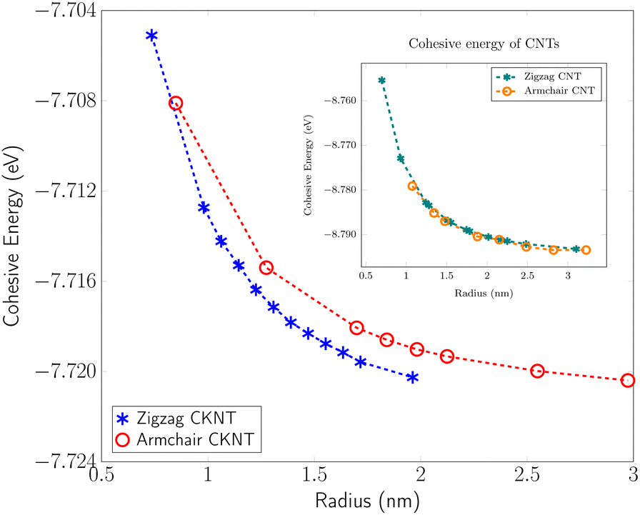 | ||
| Fig. 4 Cohesive energy of zigzag and armchair CKNTs. Inset: Cohesive energy of conventional zigzag and armchair carbon nanotubes (CNTs) presented for comparison. | ||
From Fig. 4, it is also evident that for a similar value of the radius, CNTs are energetically more favorable compared to CKNTs (i.e., CNTs have larger cohesive energies). We remark however that this observation in of itself does not preclude the synthesis of CKNTs. Indeed, fullerenes can be readily produced, although they have long been known to have cohesive energies that are somewhat lower than other common allotropes of carbon.104,149–151 More recently γ-graphyne, which has a significantly lower cohesive energy compared to graphene152 has also been chemically synthesized.153–155 Notably, there has also been success in synthesis of other unusual quasi-one-dimensional allotropes of carbon starting from conventional carbon nanotubes,73 which may be adopted for producing CKNTs.
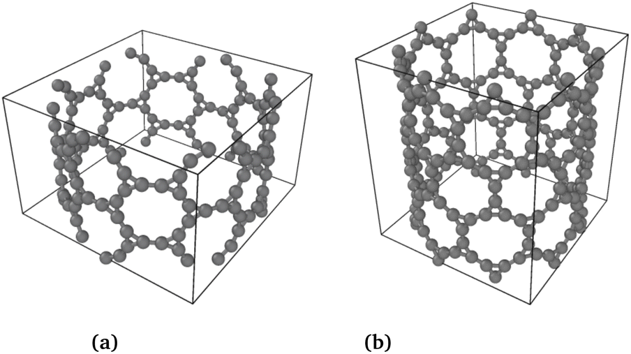
The phonon stability of Kagome graphene sheets has been investigated earlier.41 Based on band-folding considerations,156–158 such calculations are also likely to be indicative of the stability of CKNTs at zero temperature. To investigate the finite temperature structural stability of CKNTs, we carried out AIMD simulations at three different temperatures—315.77 K, 631.54 K and 947.31 K. The system energy is observed to be stable throughout each of these simulations (Fig. 7). We conclude that CKNTs are able to maintain their overall structural integrity at room temperature, and beyond, thus making them physically realistic nanostructures. Notably, during the course of the simulations, the structures appear to undergo dynamic distortions similar to conventional CNTs,105,159,160 and show a propensity for developing transitory ellipsoidal cross sections, especially at elevated temperature (Fig. 6a). Nevertheless, the dodecagonal rings which make up CKNTs and which are crucially related to their fascinating electronic properties (discussed in Section 3.3), continue to be maintained (Fig. 6b). Given the relatively low sheet bending stiffness of Kagome graphene (as compared to conventional graphene, e.g.), it is quite possible that large diameter CKNTs, like their CNT counterparts161–163 have a tendency to collapse. From this perspective, the distorted cross sections described above are possible indicators of this kind of structural transition, and warrant further investigation in the future. Snapshots of the AIMD simulations is provided in Fig. 5, 6, and the entire simulation trajectories at 315.77 K are available as ESI.†
 | ||
| Fig. 5 Snapshot of AIMD simulations at 315.77 K for both types of CKNTs. | ||
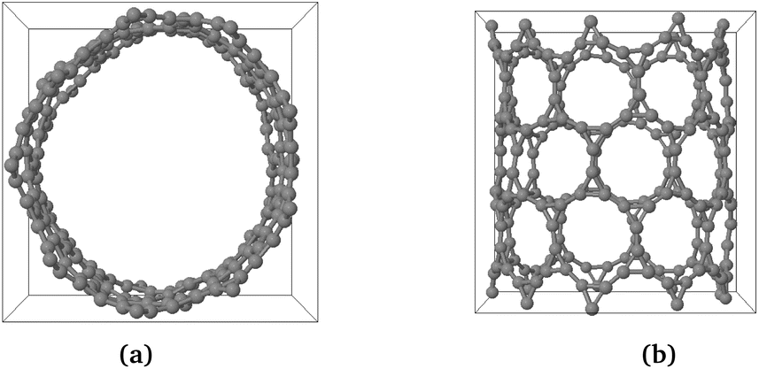 | ||
| Fig. 6 Snapshot of AIMD simulations of a zigzag CKNT at an elevated temperature of 631.554 K. The cross-section shows a propensity for developing transitory distortions (left image). However, the overall structural integrity and the 12-fold rings continue to be maintained (right image). | ||
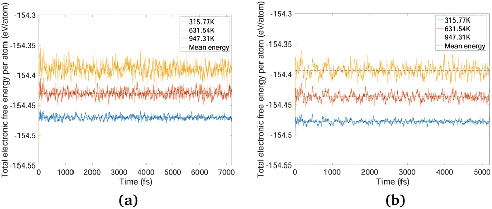 | ||
| Fig. 7 System energy variation over ab initio molecular dynamics (AIMD) trajectories at three different temperatures for (a) an Armchair CKNT and (b) a zigzag CKNT. The AIMD simulations reveal that the nanotubes maintains their overall structural integrity far above room temperature. | ||
3.2 Mechanical properties: torsional and extensional stiffness
We focus on mechanical properties of CKNTs, namely their torsional and extensional responses in the linear elastic regime. As described earlier, Helical DFT allow such calculations to be carried out by introducing changes in the nanotube symmetry group parameters. We consider (12,12) armchair (radius 1.7 nm) and (12,0) zigzag (radius 0.98 nm) CKNTs as representative examples. For both these tubes, we start from the undistorted, relaxed configurations.For simulations involving torsion, we increment the parameter α in regular intervals, imposing up to about β = 4.5° of twist per nanometer, the limit of linear response for conventional CNTs.105 For each twisted configuration, we relax the atomic forces and compute the twisting energy per unit length of the nanotubes as the difference in the ground state free energy (per fundamental domain) of the twisted and untwisted structures, i.e.:
 | (5) |
In the equation above,  and
and  denote the symmetry groups associated with the twisted and untwisted structures, respectively and (as before)
  denotes the cyclic group order. Additionally,
  and
and  denote the collections of relaxed positions of the atoms in the fundamental domain in each case. Thereafter, the torsional stiffness is computed as:
 | (6) |
We observed that for the range of torsional deformations considered here, the behavior of Utwist(β) is almost perfectly quadratic with respect to β, consistent with linear elastic response (see Fig. 8). Moreover, the value of ktwist is estimated to be 3156.1 eV/nm and 979.51 eV/nm for the armchair and zigzag tubes, respectively. In the linear elastic regime, the torsional behavior of nanotubes is well approximated by continuum models which suggest that ktwist should vary with the tube radius in a cubic manner.99,105,164 By use of this scaling law, we were able to estimate that conventional CNTs with radii comparable to the CKNTs considered above are expected to be significantly more rigid with respect to twisting (with ktwist values equal 2.8977 × 10⁴ eV/nm and 5525.0 eV/nm for 1.7 nm and 0.98 nm radius conventional CNTs, respectively).
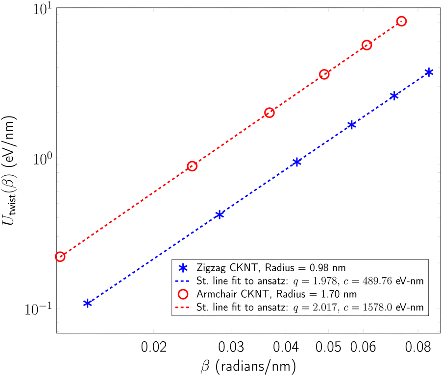 | ||
| Fig. 8 Twist energy per unit length as a function of angle of twist per unit length for two representative nanotubes (both axes logarithmic). Dotted lines indicate straight line fits of the data to an ansatz of the form Utwist(β) = c × βq. The exponent q is nearly 2 in both cases, suggesting linear elastic behavior. | ||
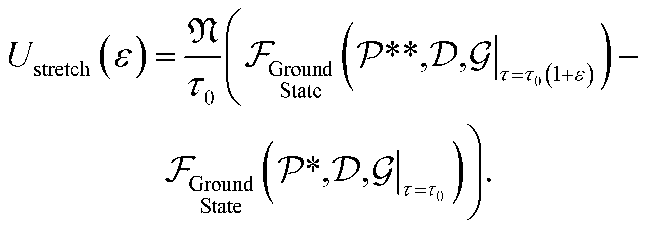
Next, for simulations involving axial stretch and compression, we proceed in a manner similar to the torsion simulations. For a given value of axial strain ε, we modify the pitch of the helical symmetry group as τ = τ0(1 + ε), with τ0 denoting the equilibrium, undistorted values. Subsequent to this kinematic prescription, we relax the atomic forces, and compute the extensional energy per unit length of the nanotubes as the difference in the ground state free energy per fundamental domain, between stretched and unstretched structures, i.e.:
 | (7) |
In the equation above,  and
and  denote the symmetry groups associated with the stretched and unstretched structures, respectively. Additionally,
  and
and  denote the collections of relaxed positions of the atoms in the fundamental domain in each case. The stretching stiffness of the nanotubes may be then calculated as:
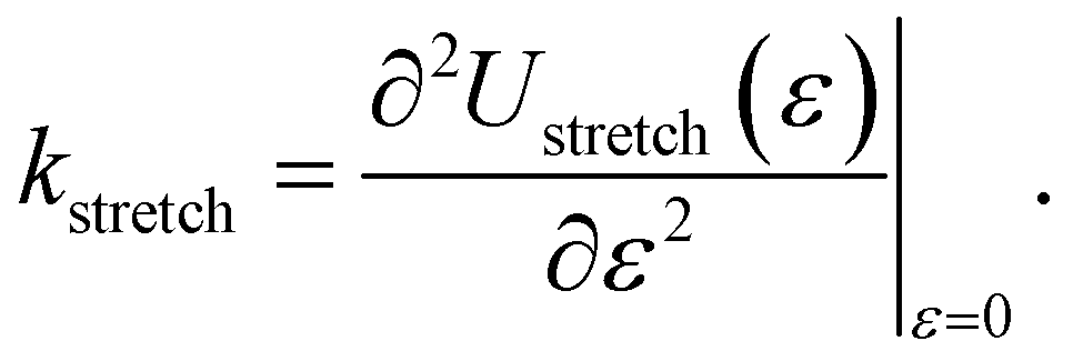 | (8) |
In our simulations, we restricted ε to be between +3.6% and −3.6%. In this range, Ustretched(ε) is found to depend in a quadratic manner on ε, consistent with linear elastic behavior (see Fig. 9). We also observed a small Poisson effect, which we have ignored in subsequent analyses. For armchair (12,12) and zigzag (12,0) CKNTs, we estimated kstretch to be 5220.9 eV/nm and 2093.4 eV/nm respectively. Based on scaling laws arising from continuum theory,164 we also estimated that conventional armchair CNTs with the same radii as the CKNTs considered above would be noticeably stiffer to axial deformations (kstretch values equal to 1.2213 × 10⁴ eV/nm and 7048.2 eV/nm for 1.7 nm and 0.98 nm radius conventional CNTs, respectively).
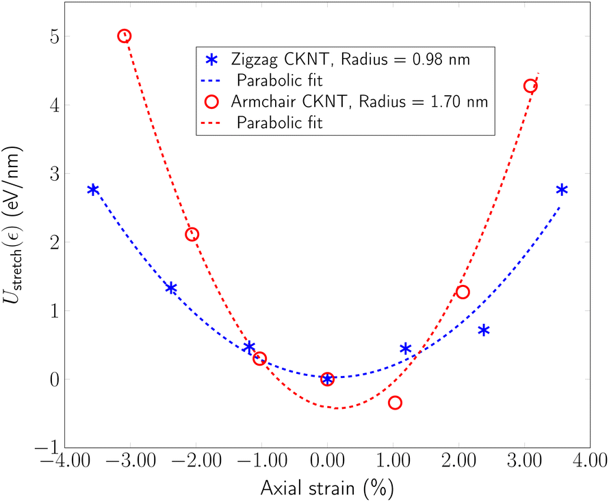 | ||
| Fig. 9 Extensional energy per unit length as a function of axial strain for two representative CKNTs. Dotted curves indicate parabolic fits of the data to an ansatz of the form Ustretch(ε) = c × ε2. | ||
Overall, these results suggest that CKNTs are significantly more pliable with respect to torsional and axial deformations, as compared to their conventional CNT counterparts. Coupled with the lower bending stiffness of Kagome graphene as compared to conventional graphene, they are indicative of the fact that Kagome graphene has a lower value of in-plane (thickness normalized) Young's modulus and shear modulus.
3.3 Electronic properties
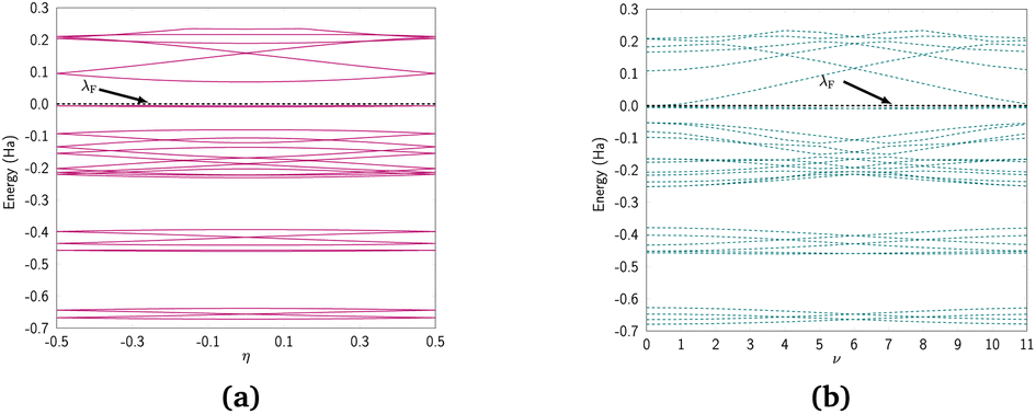
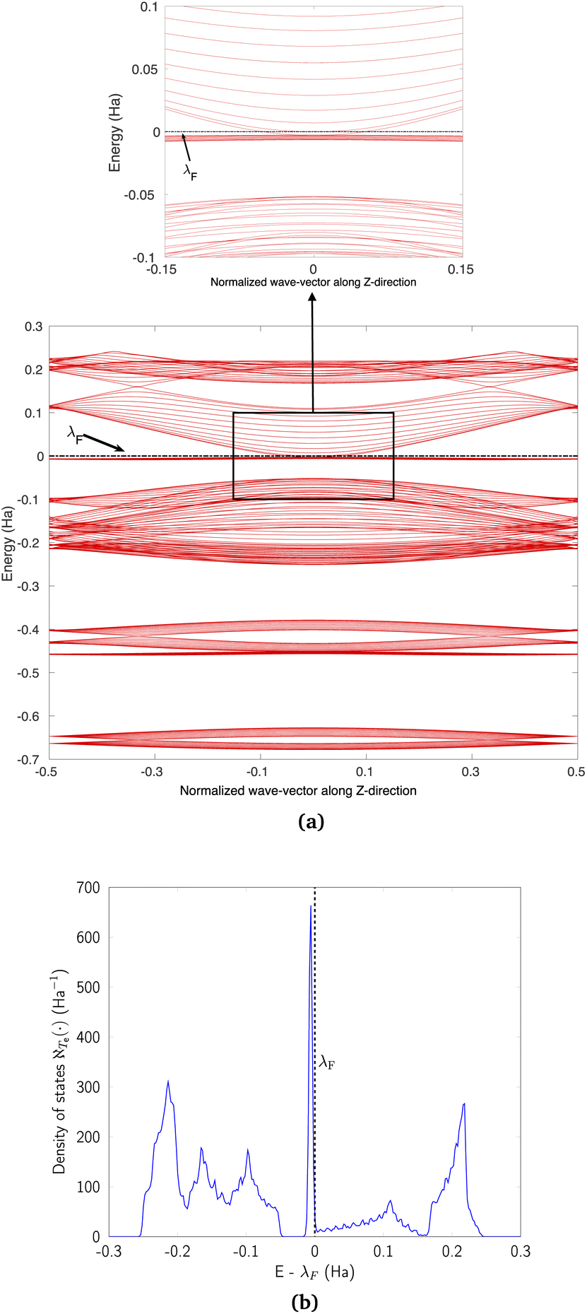
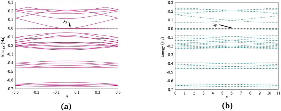
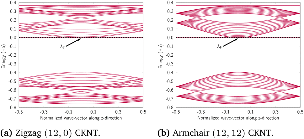
We discuss the electronic properties of CKNTs as revealed by first principles simulations. We start from a discussion of the properties of undistorted tubes, following which we discuss the electronic response of the tubes when subjected to torsional and axial strains. In A we describe a symmetry adapted tight-binding (TB) model that is able to explain these electronic properties. divisible by 3 are metallic), and the electronic band diagrams of these materials prominently feature Dirac points near the Fermi level.99,100,104,129,165 In contrast, our simulations reveal all CKNTs to be metallic, with their electronic band diagrams prominently featuring dispersionless electronic states, or flat bands, close to the Fermi level. Fig. 10a and 12a show complete band diagrams of undistorted CKNTs (i.e., all electronic states corresponding to allowable values of reciprocal space parameters η, ν are plotted), while Fig. 11 and 13 show symmetry adapted versions of these plots (i.e., band diagrams with chosen reciprocal space parameters along cyclic or helical directions). Notably, a CKNT of cyclic group order
  is found to feature
  nearly degenerate flat bands near the Fermi level. An associated singular peak in the electronic density of states (Fig. 10b and 12b) is also observed,|| and both zigzag and armchair tubes are found to feature quadratic band crossing (QBC) points at η = 0 (corresponding to the gamma point of the flat sheet). These features make CKNTs striking examples of realistic quasi-one-dimensional materials that are likely to exhibit strongly correlated electronic states. The detailed investigation of exotic materials phenomenon in CKNTs resulting from such strong electronic correlations—including e.g., Wigner crystallization, flat-band ferromagnetism and the emergence of superconducting, nematic or topological phases41,166,167—is the scope of future work. Considering that such phenomena have been studied primarily in bulk and two dimensional materials, the role that the quasi-one-dimensional morphology of CKNTs might play in them makes these investigations particularly interesting.
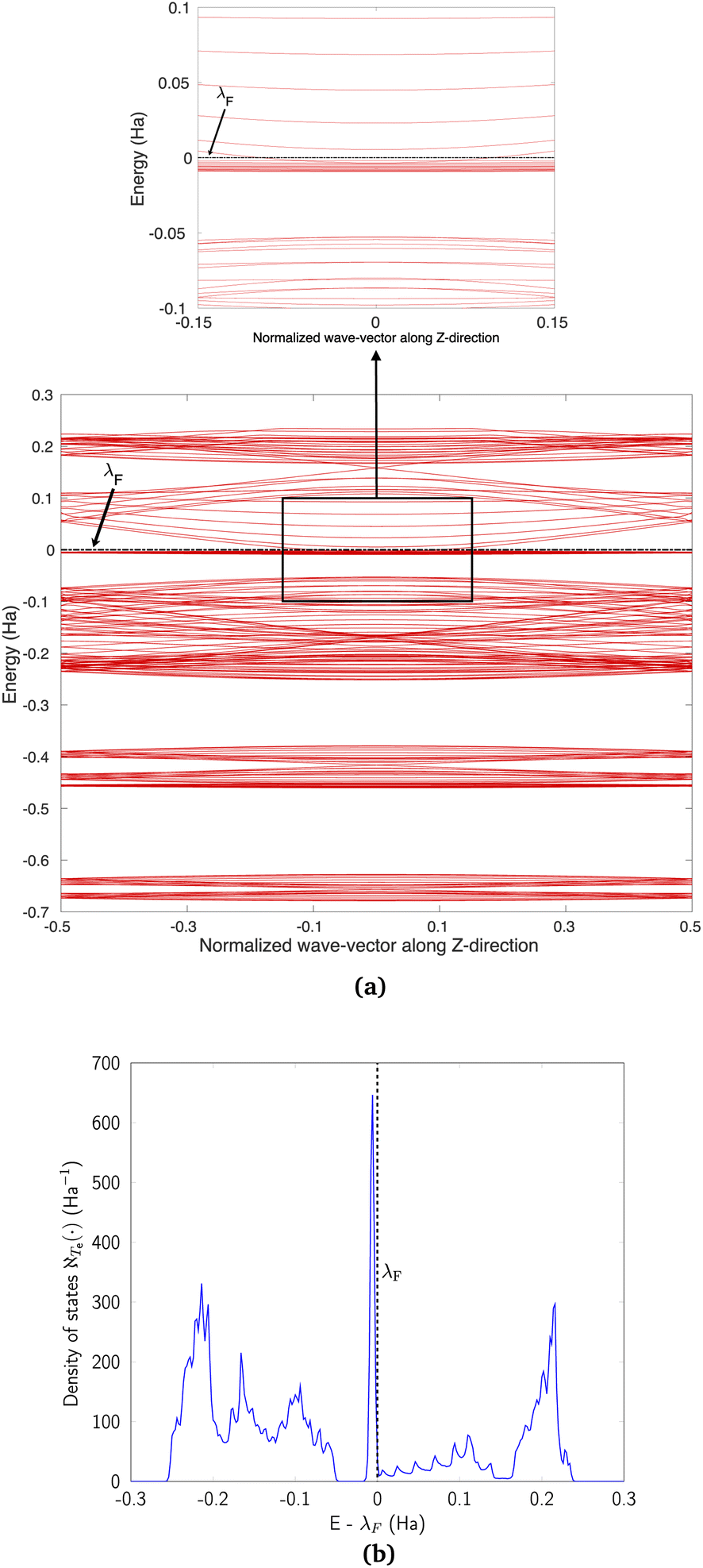 | ||
| Fig. 10 (a) Complete band diagram and (b) electronic density of states near the Fermi level of an undistorted zigzag CKNT (radius 0.98 nm). λF denotes the Fermi level. | ||
 | ||
| Fig. 11 Symmetry adapted band diagrams of an undistorted zigzag CKNT (radius 0.98 nm) obtained using Helical DFT.98,99 λF denotes the Fermi level. | ||
 | ||
| Fig. 12 (a) Complete band diagram and (b) electronic density of states near the Fermi level for the undistorted armchair CKNT (radius 1.70 nm). λF denotes the Fermi level. | ||
 | ||
| Fig. 13 Symmetry adapted band diagrams of an undistorted armchair CKNT (radius 1.70 nm) obtained using Helical DFT.98,99 λF denotes the Fermi level. | ||
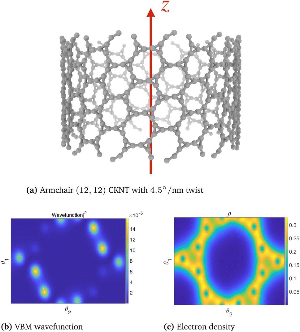
The dispersionless states in CKNTs are caused by destructive interference, resulting from geometric and orbital frustration, as has also been shown to occur in other Kagome lattice systems.168–170 The electron effective mass is arbitrarily large at the flat band and the diminished electronic kinetic energy allows the Coulombic interactions to dominate, resulting in strong electronic correlation. In turn, this causes electron localization** and the emergence of a sharp peak (i.e., van Hove singularity173) in the electronic density of states (DOS) near the Fermi level (as shown in Fig. 10b and 12b). The localized states corresponding to an undistorted armchair CKNT are shown in Fig. 14a. A plot of the electron density distribution for that system is also shown (Fig. 14b).
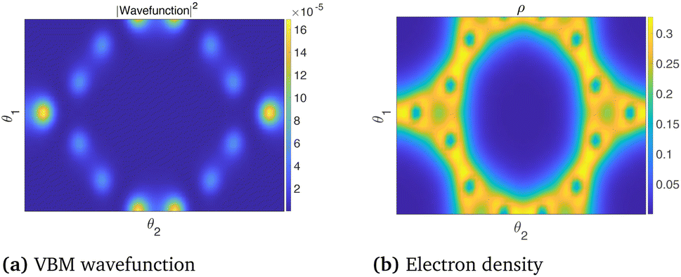 | ||
| Fig. 14 Valence Band Maximum (VBM) wavefunction and the electron density of an undeformed armchair (12,12) CKNT. A slice of the electronic fields at the average radial coordinate of the atoms in the computational domain (represented using helical coordinates98) is shown. | ||
At this point, it is worth mentioning some similarities of the electronic properties of CKNTs with their conventional counterparts. Like conventional CNTs, the fascinating electronic properties of CKNTs are largely connected to π electrons formed from radially oriented pz orbitals, while the px and py orbitals form in-plane σ bonds and are largely electronically inactive.41 This is supported by projected density of states (PDOS) calculations for CKNTs (Fig. 15), which show that the singular peak in the (total) electronic density of states near the Fermi level is largely attributable to the contributions of the individual (radially oriented) pz (l = 1, ml = 0) orbitals, while px and py orbital contributions lie well below the Fermi level. Moreover, the band diagrams of CKNTs have some similarities in appearance with those of conventional CNTS, e.g., the presence of Dirac points at η = 0 for zigzag tubes and at  for armchair ones (Fig. 10aand 12a). However, unlike conventional CNTs, these Dirac points do not appear at the Fermi level in undistorted CKNTs, but are prominently featured as a part of the excited states of the system.
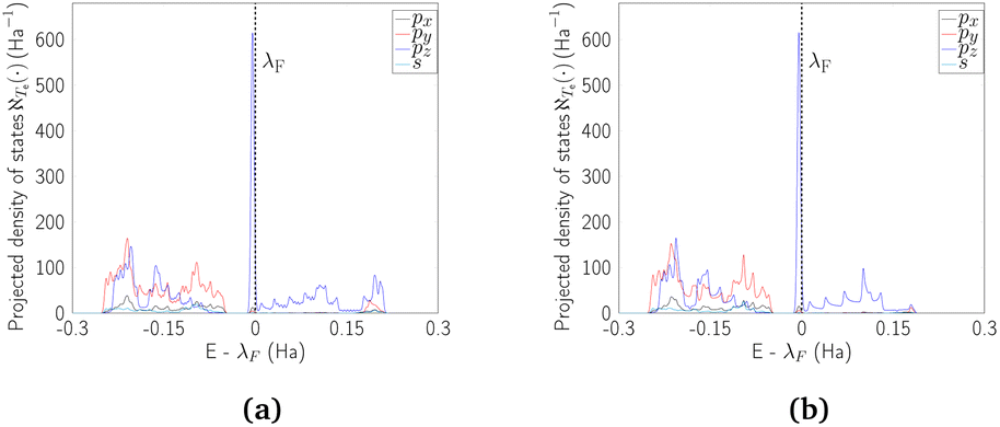 | ||
| Fig. 15 Projected density of states (PDOS) for undistorted armchair and zigzag CKNTs. The largest contribution to the sharp peak near the Fermi level is seen to arise from pz orbitals. | ||
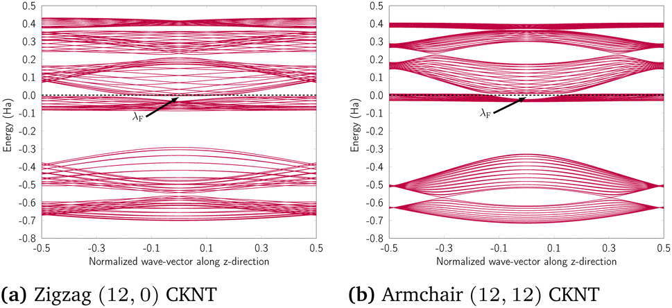
 flat bands at the Fermi level appear to be lifted, and a number of dispersionless states appear to give way to bands that are only partially flat. The change of completely flat bands to ones which have some dispersion near η = 0 is also evidenced by the electronic density of states plot in Fig. 17b, which shows that the sharp peak near the Fermi level decays as the rate of applied twist increases. Despite these twist induced changes, a number of dispersionless states survive (Fig. 16a) and spatially localized wavefunctions associated with such states continue to be hosted by the nanotube (Fig. 16b). Notably, the application of twist results in energy dispersion relations that feature rather dramatic changes in the electronic effective mass as the Brillouin zone is traversed—from infinitely massive carriers near η = 0, to massless ones as the Dirac points are reached, and then re-appearance of infinitely massive ones as the edge of the Brillouin zone is approached (i.e., closer to
  ). Overall, these observations suggest that torsional strains provide a way of controlling correlated electronic states in CKNTs. Moreover, twisted CKNTs, being chiral, are likely to show asymmetric transport properties.51,52 Therefore, they provide an interesting, realistic material platform where the combined manifestations of anomalous transport phenomena (the Chiral Induced Spin Selectivity effect178) and flat band physics may be realized and studied.
 | ||
| Fig. 16 Atomic configuration, Valence Band Maximum (VBM) wavefunction and the electron density of an armchair (12,12) CKNT with β = 4.5° nm applied twist. A slice of the electronic fields at the average radial coordinate of the atoms in the computational domain (represented using helical coordinates98) is shown. | ||
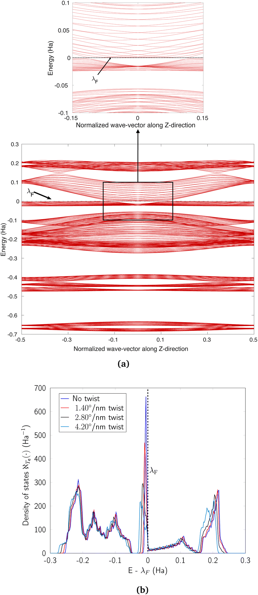 | ||
| Fig. 17 (a) Complete band diagram and (b) electronic density of states near the Fermi level for the twisted armchair CKNT (radius 1.70 nm). λF denotes the Fermi level. | ||
Next, we discuss the case of axial strains. In general, such deformations also tend to introduce some degree of dispersion into the flat bands of CKNTs near η = 0, while lifting their degeneracies near the Fermi level. However, their influence appears to be less dramatic than the case of torsional deformations described above. Nevertheless, the axial compression case deserves particular mention. Considering the zigzag (12,0) CKNT for example, we observe (see Fig. 18a) that the dispersion introduced in the flat bands near η = 0 results in curvature of these states in a manner that is opposite (i.e., convex vs. concave) of the situation encountered while twist is applied (i.e., Fig. 17a). Thus, a scenario akin to the touching of a pair of parabolic bands176,179 emerges. Upon subjecting the tube to larger values of compression, we observed that the parabolic bands near η = 0 give way to linear dispersion, i.e., the emergence of Dirac points. Commensurate with these changes, the sharp peak in electronic the density of states (Fig. 18b) also diminishes with increasing magnitude of axial strain, although the decrease appears to be less dramatic than the situation encountered with torsion (i.e., Fig. 17b).
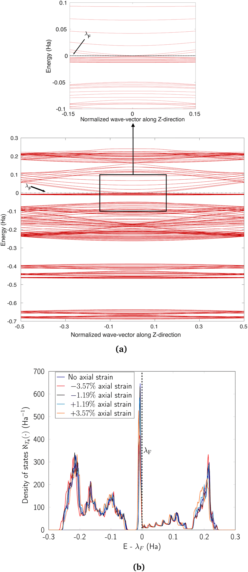 | ||
| Fig. 18 (a) Complete band diagram and (b) electronic density of states near the Fermi level for the stretched zigzag CKNT (radius 0.98 nm). λF denotes the Fermi level. | ||
Overall, the above observations are consistent with literature that suggests that quadratic band crossing points are unstable with respect to strains.180,181 It is also worthwhile at this point to contrast the electromechanical response of CKNTs to conventional CNTS. Zigzag CNTs with cyclic group order divisible by 3 and armchair CKNTs are both metallic,100 and they are known to be more sensitive to axial and torsional strains respectively. The effect of such deformations, at least for small strains, is to open up a gap at the Dirac points of these materials, resulting in metal–semiconductor transitions.99,165,182–185 As described above, CKNTs appear to show more dramatic electronic transitions when subjected to such strains. At the same time, the simulations above suggest that at least some dispersionless states in CKNTs are robust and continue to be available when the tube is subjected to small torsional and axial strains.
3.4 Possible routes to the synthesis of CKNTs
Our calculations suggest that CKNTs are kinetically stable, which is often taken to be a promising sign of the synthesizability of carbon allotropes.41,188 In the past, a wide variety of metastable carbon allotropes have been fabricated,189 often with significantly lower cohesive energies than other common stable counterparts. Examples of successful synthesis of such unusual carbon allotropes include γ-graphyne,152–155 T-carbon73,190 and nitrogen-doped Kagome graphene.93,94 In particular, various methods of synthesis of conventional carbon nanotubes, including laser ablation and chemical vapor deposition have been explored.191,192 Some of these techniques have also been successfully used in manufacturing other 1D carbon allotropes, e.g. T-carbon nanotubes, which can be created from conventional carbon nanotubes through a picosecond pulsed-laser irradiation induced first order phase transition. Such techniques provide additional routes for synthesizing CKNTs. Irrespective of the method, we anticipate that the analysis presented in this paper is likely to be instrumental in realizing CKNTs experimentally.Since a variety of routes have been exploited for synthesizing different allotropes of carbon, multiple avenues also possibly exists for realizing CKNTs. We suggest two possibilities here, both based on the organic synthesis of Kagome graphene and subsequent roll-up of this material to form CKNTs. One possibility is to use silver adatoms to transform tetrabromobocyclopropene to intermediate organometallic complex and to then form Kagome graphene on the surface of SiO2 substrate with etchant sensitive gold layer in between ,93 as represented in left panel of Fig. 19a. The second possibility is through the use of cyclopropane or bicyclopropane,41,188 wherein tailoring of ligand chemistry can be used to form self-assembled kagome graphene on the surface of gold (111), deposited on a SiO2 substrate (shown in right panel of Fig. 19a). This latter method is similar to recently demonstrated self-assembly procedures in metastable carbon nanowiggles.193,194 After the synthesis of Kagome graphene, targeted etching of the gold layer195 can result in the curling of the 2D material into CKNTs, as desired. The lower bending stiffness of kagome graphene in contrast to conventional graphene (Section 3.1) will likely assist in this step (Fig. 19b).
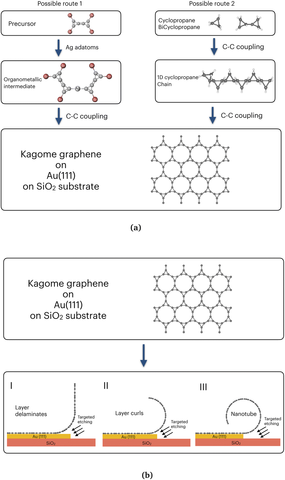 | ||
| Fig. 19 Possible routes of synthesis of CKNTs. (a) Two possible routes to synthesis Kagome graphene. (b) Rolling up of a layer of Kagome graphene by target itching to form CKNTs. | ||
4 Conclusion
In summary, we have introduced carbon Kagome nanotubes (CKNTs)—a new allotrope of carbon formed through a roll-up construction of Kagome graphene. These nanotubes are unique in the sense that contemporarily, they are perhaps the only known example of realistic, elemental, 1D nanostructures that can host dispersionless electronic states, or flat bands, in the entirety of their (one-dimensional) Brillouin zone. They also feature Dirac points in their band diagram, as well as a singular peak in their electronic density of states. Thus, they provide an attractive platform for studying and exploiting strongly correlated electronic phenomena in nanomaterials with wire-like geometries.To characterize CKNTs, we have carried out an extensive series of first principles simulations, including specialized calculations based on symmetry adaptation. We have investigated both zigzag and armchair varieties of CKNTs. Cohesive energy computations and ab initio molecular dynamics simulations suggest CKNTs should exist as stable structures at room temperature and beyond. Our simulations reveal that it is easier to roll Kagome graphene into CKNTs than it is to roll conventional graphene into CNTs. Moreover, CKNTs are found to be significantly more pliable with respect to torsional and extensional deformation as compared to CNTs of similar radii. Both zigzag and armchair varieties of CKNTs are found to be metallic, and are seen to feature multiple degenerate flat bands and a corresponding singular peak in the electronic density of states, near the Fermi level. We studied the response of electronic properties of CKNTs to applied torsional and axial strains and showed that such deformations are very effective in inducing large changes in the electronic states of this material. We also developed a tight binding model which is able to capture many of the electronic properties of CKNTs observed in first principles calculations, and also reproduces correctly, the effect of strains in the material.
Given the relative stability of CKNTs and the fact that there has been recent successes in experimentally synthesizing various novel carbon allotropes, it appears likely that CKNTs can be produced and studied under laboratory conditions in the near future. Such pursuits, as well as more detailed characterizations of electronic phenomena in CKNTs at a level beyond Density Functional Theory, and the exploration of anomalous transport phenomena in distorted CKNTs, are all attractive directions of future research.
A Appendix: tight binding model for CKNTs
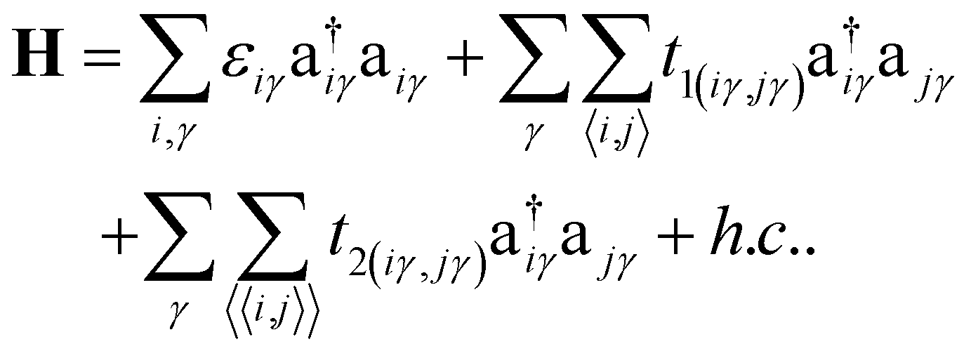
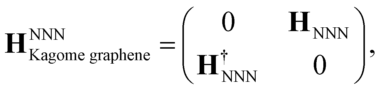
We have developed a pπ-orbital based tight-binding (TB) model for understanding the electronic structure of CKNTs. As described below, to correctly reproduce the findings of the ab initio calculations, especially the effects of strain, we found it necessary to include up to next–nearest–neighbor (NNN) interactions and to make the hopping amplitudes dependent on relative changes in bond lengths. The TB Hamiltonian in second quantization framework196,197 is written as:
 | (9) |
 , respectively. The onsite energy, εiγ, is considered zero for convenience. To calculate the TB band structure of CKNTs, we adopt the Dresselhaus method.104 This procedure involves development of a TB formulation for the flat sheet (i.e., Kagome graphene), and subsequent mapping of the atoms of the two-dimensional lattice to a cylinder, so as to invoke boundary conditions appropriate to the nanotube. Details of these steps are discussed below.
Results from our TB calculations are presented in Fig. 20 and 21. As can be seen, there is excellent qualitative agreement between these results and the first principles data presented earlier.
 | ||
| Fig. 20 Band diagram of undistorted CKNTs obtained from the tight binding model: (a) Armchair and (b) zigzag cases shown. λF denotes the Fermi level. | ||
 | ||
| Fig. 21 Band diagram of twisted CKNTs obtained from the tight binding method, with about 4.8° nm−1 of applied twist. λF denotes the Fermi level. | ||
A.1 Tight binding model for Kagome graphene
The hexagonal unit cell of Kagome graphene consist of two triangular sublattices A and B (Fig. 22), consisting of a total of six carbon atoms per unit cell. We consider only pz orbitals in the TB method which yield a 6 × 6 TB hamiltonian, written in momentum space for NN interactions as:41
 | (10) |
 | ||
| Fig. 22 Kagome graphene structure with two sublattices A and B consisting of total six carbon atoms in the unit cell. | ||
Axial or torsional strains in CKNTs can be mapped to appropriate deformations in Kagome graphene. For example, torsional strains in CKNTs have the effect of inducing a shear strain in the underlying Kagome graphene lattice. Generally, such distortions transform the sublattices in Kagome graphene from being perfect equilateral triangles to scalene triangles, so that the hopping matrix of sublattices B will no longer be the Hermitian conjugate of that of sublattices A. The NN hopping matrix HAA of the sublattice A can be written as (refer to Fig. 22):
 | (11) |
while the inter-triangular hopping matrix HAB can be written as:
 | (12) |
The matrices HBB and HBA can be written in the similar manner, and are not shown here for brevity. Consistent with the geometry of Kagome graphene and the mapping of strains from CKNTs to the Kagome graphene lattice, we choose a1 = [1, 0, 0], a2 = [cos(θ0 + 2πα), sin(θ0 + 2πα), 0] and a3 = a1 − a2 as the unit vectors in real space, and we further set 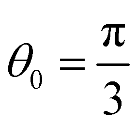 . We denote k = [kx, ky] as the unit vector in reciprocal space.
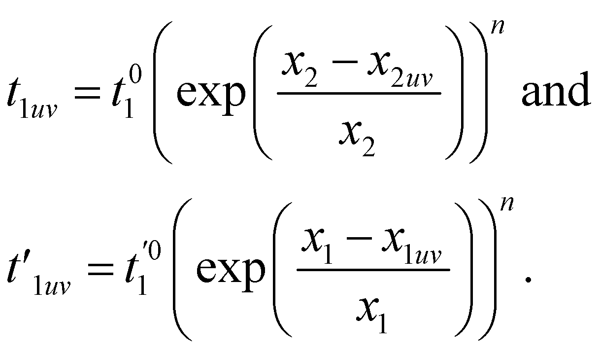
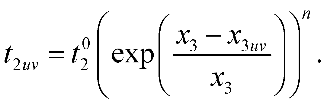
The hopping amplitudes depend on the structure of the lattice and the applied deformations, and can be written as the function of relative change in bond length:198
 | (13) |
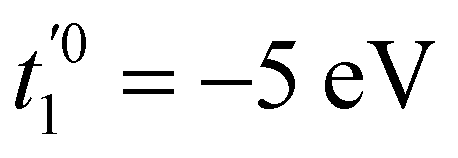 , t01 = −7 eV are the NN hopping parameters,199 and x1 and x2 are inter- and intra-triangular bond lengths in the undeformed structure (Fig. 1). The bond lengths x2uv and x1uv are in the deformed system, and u, v run over the NN atoms as shown in Fig. 22. The parameter n controls the magnitude of the hopping parameter upon deformation of the lattice and parameterizes the “flatness” of the dispersionless states. Here, α is the nanotube's applied twist parameter, as explained earlier in section 2.2.1. Following literature,198 we use n = 8 for getting both relatively flat bands and smooth evolution of band structure upon deformation.
The NNN interactions in our TB Hamiltonian take the following form:
 | (14) |
 | (15) |
A.2 (n, m) nanotube and boundary conditions
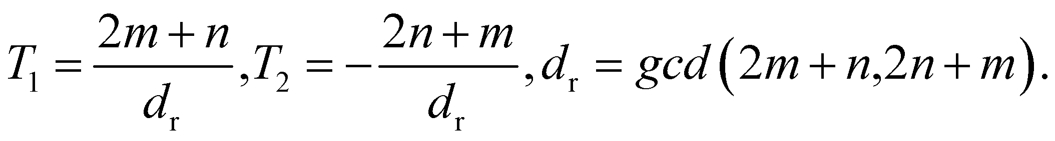
To adapt the TB model of Kagome graphene described above to CKNTs, we follow the method developed by Dresselhaus.104 The general procedure starts by considering a semi-infinite two-dimensional sheet, whereby the two opposite edge sides are glued together to form an infinite tube, with the axis of the tube chosen to be the eZ-direction. The periodicity along the circumferential direction naturally imposes periodic boundary conditions on the circumferential wave vector, denoted k⊥ below. In what follows, we briefly describe the procedure for imposing such periodic boundary conditions on a nanotube constructed from an arbitrary two-dimensional lattice. Axial and torsional deformations in the nanotube can be naturally incorporated by considering the effect of applied strains to the two-dimensional lattice.We first describe the construction of an (n, m) nanotube by rolling up a flat sheet along the direction of a chiral vector. The flat sheet is assumed to be generated using a 2D hexagonal lattice, with lattice vectors a1 and a2, each of length a0 (the lattice vectors for Kagome graphene are given in A.1 above). The chiral vector for a nanotube with chirality (n, m) is then Ch = na1 + ma2, where n, m are non-negative integers. The translation vector which is parallel to the axis of the nanotube is expressed as T = T1a1 + T2a2. Furthermore, gcd(T1, T2) = 1,  , and:
The translation vector determines the axial periodicity of the nanotube, such that in real space, the unit cell of the nanotube is described by a rectangle generated by Ch × T. The reciprocal lattice vectors corresponding to Ch and T are k⊥ and k‖, respectively. Since, Ch and Th are orthogonal vectors, this gives Ch·k⊥ = 2π, Ch·k‖ = 0, T·k⊥ = 0, and T·k‖ = 2π. By substituting k⊥ and k‖ into the orthogonality constraints, we get:
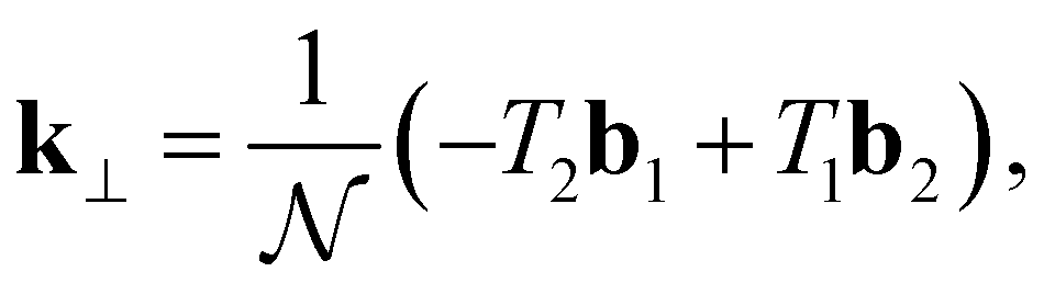 | (16) |
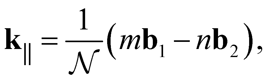 | (17) |
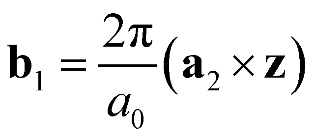 and
and 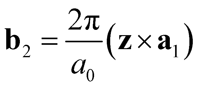 are the unit vectors of the reciprocal lattice of the two-dimensional lattice, a0 is the lattice parameter, and z is perpendicular to both a1 and a2. Furthermore,
  is the number of primitive unit cells per nanotube unit cell, and can be expressed as:
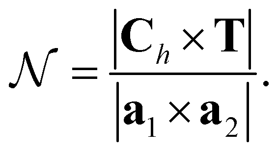 | (18) |
Note that, for the zigzag and armchair tubes considered here,  is related to the cyclic group order as
  .
.
The energy dispersion relations (i.e., electronic band diagrams) can be obtained104 by first writing the TB Hamiltonian of the flat sheet, and then applying the periodic boundary condition along the direction of chiral vector, Ch, i.e., ψ(x + Ch) = ψ(x). This leads to the condition exp(ik·Ch) = 1 and quantizes the wave vector k⊥, thus giving rise to  discrete wavevectors parallel to k⊥, in the direction of Ch. The wavevector k‖, which is parallel to the axis of the nanotube, remains continuous, however. Since the two-dimensional sheet is being rolled-up to form a quasi-one-dimensional nanotube, the Brillouin zone (BZ) is one-dimensional, and the condition T·k‖ = 2π implies that the length of the Brillouin zone is 2π/T. Thus, the
  one-dimensional energy dispersion relations for the nanotube can be parametrized as
  , with
  and
and 
Note that this construction immediately implies that a zigzag or armchair CKNT of cyclic group order  will feature
  flat bands, since the starting point is the Kagome graphene TB Hamiltonian (A.1) featuring a single flat band across its Brillouin zone. This is consistent with the observations made from first principles calculations (Section 3.3).
Author contributions
Hsuan Ming Yu: data curation, formal analysis, investigation, validation, visualization, writing – original draft. Shivam Sharma: data curation, formal analysis, investigation, validation, visualization, writing – original draft. Shivang Agarwal: data curation, investigation, writing – original draft. Olivia Liebman: investigation, writing – original draft. Amartya S. Banerjee: conceptualization, formal analysis, methodology, resources, software, supervision, validation, writing – review & editing.Conflicts of interest
There are no conflicts to declare.Acknowledgements
This work was supported by grant DE-SC0023432 funded by the U.S. Department of Energy, Office of Science. This research used resources of the National Energy Research Scientific Computing Center, a DOE Office of Science User Facility supported by the Office of Science of the U.S. Department of Energy under Contract No. DE-AC02-05CH11231, using NERSC awards BES-ERCAP0025205 and BES-ERCAP0025168. ASB acknowledges startup support from the Samueli School Of Engineering at UCLA, as well as funding from UCLA's Council on Research (COR) Faculty Research Grant. ASB also acknowledges support through a Faculty Career Development Award from UCLA's Office of Equity, Diversity and Inclusion. ASB would like to thank Felipe Jornada (Stanford Univ.), Giulia Galli (Univ. of Chicago), Garnet Chan (Caltech), Ellad Tadmor (Univ. of Minnesota), Lin Lin (Univ. of California, Berkeley), David J. Singh (Univ. of Missouri), Suneel Kodambaka (Virginina Tech.), Yves Rubin (UCLA) and Rahul Roy (UCLA) for insightful discussions and suggestions, and Neha Bairoliya (Univ. of Southern California) for providing encouragement and support, during the preparation of this manuscript. SS would like to thank Richard D. James (Univ. of Minnesota), and acknowledge financial support from MURI project grant (FA9550-18-1-0095). The authors would like to thank UCLA's Institute for Digital Research and Education (IDRE) and the Minnesota Supercomputing Institute (MSI) for making available some of the computing resources used in this work.References
- K. Novoselov, D. Jiang, F. Schedin, T. Booth, V. Khotkevich, S. Morozov and A. Geim, Proc. Natl. Acad. Sci. U. S. A., 2005, 102, 10451–10453 CrossRef CAS PubMed.
- K. Novoselov and A. Morozov, et al., Nature, 2005, 438, 197–200 CrossRef CAS PubMed.
- L. Balents, C. R. Dean, D. K. Efetov and A. F. Young, Nat. Phys., 2020, 16, 725–733 Search PubMed.
- J.-X. Yin, S. S. Zhang, G. Chang, Q. Wang, S. S. Tsirkin, Z. Guguchia, B. Lian, H. Zhou, K. Jiang and I. Belopolski, et al., Nat. Phys., 2019, 15, 443–448 Search PubMed.
- O. Derzhko, J. Richter and M. Maksymenko, Int. J. Mod. Phys. B, 2015, 29, 1530007 CrossRef.
- C. Elias, G. Fugallo, P. Valvin, C. L'Henoret, J. Li, J. Edgar, F. Sottile, M. Lazzeri, A. Ouerghi and B. Gil, et al., Phys. Rev. Lett., 2021, 127, 137401 CrossRef CAS PubMed.
- V. Iglovikov, F. Hébert, B. Grémaud, G. Batrouni and R. Scalettar, Phys. Rev. B: Condens. Matter Mater. Phys., 2014, 90, 094506 CrossRef CAS.
- R. Pons, A. Mielke and T. Stauber, Phys. Rev. B, 2020, 102, 235101 CrossRef CAS.
- C. Wu, D. Bergman, L. Balents and S. D. Sarma, Phys. Rev. Lett., 2007, 99, 070401 CrossRef PubMed.
- M. Shayegan, Nat. Rev. Phys., 2022, 4, 212–213 CrossRef.
- Y.-F. Wang, H. Yao, C.-D. Gong and D. Sheng, Phys. Rev. B: Condens. Matter Mater. Phys., 2012, 86, 201101 CrossRef.
- E. Tang, J.-W. Mei and X.-G. Wen, Phys. Rev. Lett., 2011, 106, 236802 CrossRef PubMed.
- K. Sun, Z. Gu, H. Katsura and S. D. Sarma, Phys. Rev. Lett., 2011, 106, 236803 CrossRef PubMed.
- T. Neupert, L. Santos, C. Chamon and C. Mudry, Phys. Rev. Lett., 2011, 106, 236804 CrossRef PubMed.
- E. Y. Andrei, D. K. Efetov, P. Jarillo-Herrero, A. H. MacDonald, K. F. Mak, T. Senthil, E. Tutuc, A. Yazdani and A. F. Young, Nat. Rev. Mater., 2021, 6, 201–206 CrossRef CAS.
- L. Wang, E.-M. Shih, A. Ghiotto, L. Xian, D. A. Rhodes, C. Tan, M. Claassen, D. M. Kennes, Y. Bai and B. Kim, et al., Nat. Mater., 2020, 19, 861–866 CrossRef CAS PubMed.
- Y. Cao, V. Fatemi, S. Fang, K. Watanabe, T. Taniguchi, E. Kaxiras and P. Jarillo-Herrero, Nature, 2018, 556, 43–50 CrossRef CAS PubMed.
- Y. Choi, H. Kim, Y. Peng, A. Thomson, C. Lewandowski, R. Polski, Y. Zhang, H. S. Arora, K. Watanabe and T. Taniguchi, et al., Nature, 2021, 589, 536–541 CrossRef CAS PubMed.
- Y. Cao, V. Fatemi, A. Demir, S. Fang, S. L. Tomarken, J. Y. Luo, J. D. Sanchez-Yamagishi, K. Watanabe, T. Taniguchi and E. Kaxiras, et al., Nature, 2018, 556, 80–84 CrossRef CAS PubMed.
- D. Leykam, A. Andreanov and S. Flach, Adv. Phys.: X, 2018, 3, 1473052 Search PubMed.
- M. N. Huda, S. Kezilebieke and P. Liljeroth, Phys. Rev. Res., 2020, 2, 043426 CrossRef CAS.
- X. Li, Q. Li, T. Ji, R. Yan, W. Fan, B. Miao, L. Sun, G. Chen, W. Zhang and H. Ding, Chin. Phys. Lett., 2022, 39, 057301 CrossRef.
- C. Barreteau, F. Ducastelle and T. Mallah, J. Phys.: Condens. Matter, 2017, 29, 465302 CrossRef CAS.
- G. Tarnopolsky, A. J. Kruchkov and A. Vishwanath, Phys. Rev. Lett., 2019, 122, 106405 CrossRef CAS PubMed.
- C. Naud, G. Faini and D. Mailly, Phys. Rev. Lett., 2001, 86, 5104 CrossRef CAS PubMed.
- J. Vidal, R. Mosseri and B. Douçot, Phys. Rev. Lett., 1998, 81, 5888 CrossRef CAS.
- B. R. Ortiz, L. C. Gomes, J. R. Morey, M. Winiarski, M. Bordelon, J. S. Mangum, I. W. Oswald, J. A. Rodriguez-Rivera, J. R. Neilson and S. D. Wilson, et al., Phys. Rev. Mater., 2019, 3, 094407 CrossRef CAS.
- M. Li, Q. Wang, G. Wang, Z. Yuan, W. Song, R. Lou, Z. Liu, Y. Huang, Z. Liu and H. Lei, et al., Nat. Commun., 2021, 12, 1–8 CrossRef.
- M. Kang, L. Ye, S. Fang, J.-S. You, A. Levitan, M. Han, J. I. Facio, C. Jozwiak, A. Bostwick and E. Rotenberg, et al., Nat. Mater., 2020, 19, 163–169 CrossRef CAS PubMed.
- E. Liu, Y. Sun, N. Kumar, L. Muechler, A. Sun, L. Jiao, S.-Y. Yang, D. Liu, A. Liang and Q. Xu, et al., Nat. Phys., 2018, 14, 1125–1131 Search PubMed.
- D. Liu, A. Liang, E. Liu, Q. Xu, Y. Li, C. Chen, D. Pei, W. Shi, S. Mo and P. Dudin, et al., Science, 2019, 365, 1282–1285 CrossRef CAS.
- T. Neupert, M. M. Denner, J.-X. Yin, R. Thomale and M. Z. Hasan, Nat. Phys., 2022, 18, 137–143 Search PubMed.
- Y.-X. Jiang, J.-X. Yin, M. M. Denner, N. Shumiya, B. R. Ortiz, G. Xu, Z. Guguchia, J. He, M. S. Hossain and X. Liu, et al., Nat. Mater., 2021, 20, 1353–1357 CrossRef CAS PubMed.
- T.-H. Han, M. Norman, J.-J. Wen, J. A. Rodriguez-Rivera, J. S. Helton, C. Broholm and Y. S. Lee, Phys. Rev. B, 2016, 94, 060409 CrossRef.
- H. Liu, S. Meng and F. Liu, Phys. Rev. Mater., 2021, 5, 084203 CrossRef CAS.
- C. Zhong, Y. Xie, Y. Chen and S. Zhang, Carbon, 2016, 99, 65–70 CrossRef CAS.
- C. Zhong, Y. Xie, Y. Chen and S. Zhang, Carbon, 2016, 99, 65–70 CrossRef CAS.
- O. Leenaerts, B. Schoeters and B. Partoens, Phys. Rev. B: Condens. Matter Mater. Phys., 2015, 91, 115202 CrossRef.
- B. Sarikavak-Lisesivdin, S. B. Lisesivdin, E. Ozbay and F. Jelezko, Chem. Phys. Lett., 2020, 760, 138006 CrossRef CAS PubMed.
- Y. Chen, Y. Y. Sun, H. Wang, D. West, Y. Xie, J. Zhong, V. Meunier, M. L. Cohen and S. B. Zhang, Phys. Rev. Lett., 2014, 113, 085501 CrossRef CAS PubMed.
- Y. Chen, S. Xu, Y. Xie, C. Zhong, C. Wu and S. B. Zhang, Phys. Rev. B, 2018, 98, 035135 CrossRef CAS.
- D. M. Kennes, L. Xian, M. Claassen and A. Rubio, Nat. Commun., 2020, 11, 1–8 CrossRef PubMed.
- Y. Li, Q. Yuan, D. Guo, C. Lou, X. Cui, G. Mei, H. Petek, L. Cao, W. Ji and M. Feng, Adv. Mater., 2023, 2300572 CrossRef CAS PubMed.
- G. R. Schleder, M. Pizzochero and E. Kaxiras, J. Phys. Chem. Lett., 2023, 14(39), 8853–8858 CrossRef CAS PubMed.
- P. C. Hohenberg, Phys. Rev., 1967, 158, 383–386 CrossRef CAS.
- N. D. Mermin and H. Wagner, Phys. Rev. Lett., 1966, 17, 1133 CrossRef CAS.
- K. Arutyunov, D. Golubev and A. Zaikin, Phys. Rep., 2008, 464, 1–70 CrossRef.
- R. Martin, L. Reining and D. Ceperly, Interacting Electrons: Theory and Computational Approaches, Cambridge University Press, 2016 Search PubMed.
- R. D. James, J. Mech. Phys. Solids, 2006, 54, 2354–2390 CrossRef.
- J. M. Kim, M. F. Haque, E. Y. Hsieh, S. M. Nahid, I. Zarin, K.-Y. Jeong, J.-P. So, H.-G. Park and S. Nam, Adv. Mater., 2022, 2107362 Search PubMed.
- C. D. Aiello, M. Abbas, J. Abendroth, A. S. Banerjee, D. Beratan, J. Belling, B. Berche, A. Botana, J. R. Caram, L. Celardo, et al., arXiv, 2020, preprint, arXiv:2009.00136, 4989–5035 Search PubMed.
- R. Naaman and D. H. Waldeck, Annu. Rev. Phys. Chem., 2015, 66, 263–281 CrossRef CAS PubMed.
- R. Nakajima, D. Hirobe, G. Kawaguchi, Y. Nabei, T. Sato, T. Narushima, H. Okamoto and H. Yamamoto, Nature, 2023, 613, 479–484 CrossRef CAS PubMed.
- J. Linder and J. W. Robinson, Nat. Phys., 2015, 11, 307–315 Search PubMed.
- A. Sidorenko, Superconducting Spintronics, Springer International Publishing, Cham, Switzerland, 2018 Search PubMed.
- F. Qin, W. Shi, T. Ideue, M. Yoshida, A. Zak, R. Tenne, T. Kikitsu, D. Inoue, D. Hashizume and Y. Iwasa, Nat. Commun., 2017, 8, 1–6 Search PubMed.
- A. Hirsch, Nat. Mater., 2010, 9, 868–871 CrossRef CAS PubMed.
- R.-S. Zhang and J.-W. Jiang, Frontiers, 2019, 14, 1–17 CAS.
- R. Hoffmann, A. A. Kabanov, A. A. Golov and D. M. Proserpio, Angew. Chem., Int. Ed., 2016, 55, 10962–10976 CrossRef CAS PubMed.
- Z. Li, Y. Xie and Y. Chen, Comput. Mater. Sci., 2020, 173, 109406 CrossRef CAS.
- Z. Wang, X.-F. Zhou, X. Zhang, Q. Zhu, H. Dong, M. Zhao and A. R. Oganov, Nano Lett., 2015, 15, 6182–6186 CrossRef CAS PubMed.
- Y. Chen, Y. Xie, X. Yan, M. L. Cohen and S. Zhang, Phys. Rep., 2020, 868, 1–32 CrossRef CAS.
- P. Yan, T. Ouyang, C. He, J. Li, C. Zhang, C. Tang and J. Zhong, Nanoscale, 2021, 13, 3564–3571 RSC.
- J.-Y. You, B. Gu and G. Su, Sci. Rep., 2019, 9, 1–7 CrossRef PubMed.
- X. Shi, S. Li, J. Li, T. Ouyang, C. Zhang, C. Tang, C. He and J. Zhong, J. Phys. Chem. Lett., 2021, 12, 11511–11519 CrossRef CAS PubMed.
- M. Zhou, Z. Liu, W. Ming, Z. Wang and F. Liu, Phys. Rev. Lett., 2014, 113, 236802 CrossRef PubMed.
- M. Maruyama and S. Okada, Carbon, 2017, 125, 530–535 CrossRef CAS.
- M. Endo, S. Iijima and M. S. Dresselhaus, Carbon Nanotubes, Elsevier, 2013 Search PubMed.
- S. Iijima and T. Ichihashi, Nature, 1993, 363, 603 CrossRef CAS.
- K. Wakabayashi, M. Fujita, H. Ajiki and M. Sigrist, Phys. Rev. B: Condens. Matter Mater. Phys., 1999, 59, 8271 CrossRef CAS.
- Y.-W. Son, M. L. Cohen and S. G. Louie, Phys. Rev. Lett., 2006, 97, 216803 CrossRef PubMed.
- S. Yu, W. Zheng, Q. Wen and Q. Jiang, Carbon, 2008, 46, 537–543 CrossRef CAS.
- J. Zhang, R. Wang, X. Zhu, A. Pan, C. Han, X. Li, D. Zhao, C. Ma, W. Wang, H. Su and C. Niu, Nat. Commun., 2017, 8, 683 CrossRef PubMed.
- V. R. Coluci, S. F. Braga, S. B. Legoas, D. S. Galvão and R. H. Baughman, Phys. Rev. B: Condens. Matter Mater. Phys., 2003, 68, 035430 CrossRef.
- V. Coluci, S. Braga, S. Legoas, D. Galvao and R. Baughman, Nanotechnology, 2004, 15, S142 CrossRef CAS.
- B. Kang and J. Y. Lee, Carbon, 2015, 84, 246–253 CrossRef CAS.
- V. Coluci, D. Galvao and R. Baughman, J. Chem. Phys., 2004, 121, 3228–3237 CrossRef CAS PubMed.
- B. Kang, J. H. Moon and J. Y. Lee, RSC Adv., 2015, 5, 80118–80121 RSC.
- D.-C. Yang, R. Jia, Y. Wang, C.-P. Kong, J. Wang, Y. Ma, R. I. Eglitis and H.-X. Zhang, J. Phys. Chem. C, 2017, 121, 14835–14844 CrossRef CAS.
- K. Wakabayashi, Y. Takane, M. Yamamoto and M. Sigrist, New J. Phys., 2009, 11, 095016 CrossRef.
- X. Yang and G. Wu, ACS Nano, 2009, 3, 1646–1650 CrossRef CAS PubMed.
- O. Arroyo-Gascón, R. Fernández-Perea, E. Suárez Morell, C. Cabrillo and L. Chico, Nano Lett., 2020, 20, 7588–7593 CrossRef PubMed.
- O. Arroyo-Gascón, R. Fernández-Perea, E. S. Morell, C. Cabrillo and L. Chico, Carbon, 2023, 205, 394–401 CrossRef.
- M. Koshino, P. Moon and Y.-W. Son, Phys. Rev. B: Condens. Matter Mater. Phys., 2015, 91, 035405 CrossRef.
- Z. Liu, F. Liu and Y.-S. Wu, Chin. Phys. B, 2014, 23, 077308 CrossRef.
- T. Wavrunek, Q. Peng and N. Abu-Zahra, Crystals, 2022, 12, 292 CrossRef CAS.
- A. Rüegg, J. Wen and G. A. Fiete, Phys. Rev. B: Condens. Matter Mater. Phys., 2010, 81, 205115 CrossRef.
- M. F. López and J. Merino, Phys. Rev. B, 2020, 102, 035157 CrossRef.
- M. F. López, B. J. Powell and J. Merino, Phys. Rev. B, 2022, 106, 235129 CrossRef.
- J. Merino, M. F. López and B. J. Powell, Phys. Rev. B, 2021, 103, 094517 CrossRef CAS.
- M. Chen, H.-Y. Hui, S. Tewari and V. Scarola, Phys. Rev. B, 2018, 97, 035114 CrossRef CAS.
- J.-W. Rhim, K. Kim and B.-J. Yang, Nature, 2020, 584, 59–63 CrossRef CAS PubMed.
- R. Pawlak, X. Liu, S. Ninova, P. D'astolfo, C. Drechsel, J.-C. Liu, R. Häner, S. Decurtins, U. Aschauer and S.-X. Liu, et al., Angew. Chem., 2021, 133, 8451–8456 CrossRef.
- X. Li, D. Han, T. Qin, J. Xiong, J. Huang, T. Wang, H. Ding, J. Hu, Q. Xu and J. Zhu, Nanoscale, 2022, 14, 6239–6247 RSC.
- A. Korde, B. Min, E. Kapaca, O. Knio, I. Nezam, Z. Wang, J. Leisen, X. Yin, X. Zhang and D. S. Sholl, et al., Science, 2022, 375, 62–66 CrossRef CAS PubMed.
- Y. Wang, K. Wan, F. Pan, X. Zhu, Y. Jiang, H. Wang, Y. Chen, X. Shi and M. Liu, Angew. Chem., 2021, 133, 16751–16757 CrossRef.
- A. S. Banerjee, PhD thesis, University of Minnesota, Minneapolis, 2013.
- A. S. Banerjee, J. Mech. Phys. Solids, 2021, 104515 CrossRef CAS.
- H. M. Yu and A. S. Banerjee, J. Comput. Phys., 2022, 456, 111023 CrossRef.
- S. Ghosh, A. S. Banerjee and P. Suryanarayana, Phys. Rev. B, 2019, 100, 125143 CrossRef CAS.
- A. S. Banerjee and P. Suryanarayana, J. Mech. Phys. Solids, 2016, 96, 605–631 CrossRef CAS.
- S. Pathrudkar, H. M. Yu, S. Ghosh and A. S. Banerjee, Phys. Rev. B, 2022, 105, 195141 CrossRef CAS.
- S. Agarwal and A. S. Banerjee, J. Comput. Phys., 2024, 496, 112551 CrossRef.
- G. Dresselhaus, M. S. Dresselhaus and S. Riichiro, Physical Properties of Carbon Nanotubes, World Scientific, 1998 Search PubMed.
- T. Dumitrica and R. D. James, J. Mech. Phys. Solids, 2007, 55, 2206–2236 CrossRef CAS.
- X. Gonze, J.-M. Beuken, R. Caracas, F. Detraux, M. Fuchs, G.-M. Rignanese, L. Sindic, M. Verstraete, G. Zerah, F. Jollet, M. Torrent, A. Roy, M. Mikami, P. Ghosez, J.-Y. Raty and D. Allan, Comput. Mater. Sci., 2002, 25, 478–492 CrossRef.
- A. H. Romero, D. C. Allan, B. Amadon, G. Antonius, T. Applencourt, L. Baguet, J. Bieder, F. Bottin, J. Bouchet and E. Bousquet, et al., J. Chem. Phys., 2020, 152, 124102 CrossRef CAS PubMed.
- X. Gonze, F. Jollet, F. A. Araujo, D. Adams, B. Amadon, T. Applencourt, C. Audouze, J.-M. Beuken, J. Bieder and A. Bokhanchuk, et al., Comput. Phys. Commun., 2016, 205, 106–131 CrossRef CAS.
- N. Troullier and J. L. Martins, Phys. Rev. B: Condens. Matter Mater. Phys., 1991, 43, 1993 CrossRef CAS PubMed.
- J. P. Perdew and Y. Wang, Phys. Rev. B: Condens. Matter Mater. Phys., 1992, 45, 13244–13249 CrossRef PubMed.
- J. P. Perdew, K. Burke and M. Ernzerhof, Phys. Rev. Lett., 1996, 77, 3865 CrossRef CAS PubMed.
- A. Van de Walle and G. Ceder, Phys. Rev. B: Condens. Matter Mater. Phys., 1999, 59, 14992 CrossRef CAS.
- N. Hamada, S.-i. Sawada and A. Oshiyama, Phys. Rev. Lett., 1992, 68, 1579–1581 CrossRef CAS PubMed.
- S. B. Sinnott and R. Andrews, Crit. Rev. Solid State Mater. Sci., 2001, 26, 145–249 CrossRef CAS.
- S. Roy, V. Jain, R. Bajpai, P. Ghosh, A. Pente, B. Singh and D. Misra, J. Phys. Chem. C, 2012, 116, 19025–19031 CrossRef CAS.
- B. Corry, J. Phys. Chem. B, 2008, 112, 1427–1434 CrossRef CAS PubMed.
- E. Frackowiak and F. Beguin, Carbon, 2002, 40, 1775–1787 CrossRef CAS.
- E. Frackowiak, S. Gautier, H. Gaucher, S. Bonnamy and F. Beguin, Carbon, 1999, 37, 61–69 CrossRef CAS.
- C. Nützenadel, A. Züttel, D. Chartouni and L. Schlapbach, Electrochem. Solid-State Lett., 1998, 2, 30 CrossRef.
- P. Giannozzi, S. Baroni, N. Bonini, M. Calandra, R. Car, C. Cavazzoni, D. Ceresoli, G. L. Chiarotti, M. Cococcioni, I. Dabo, A. D. Corso, S. de Gironcoli, S. Fabris, G. Fratesi, R. Gebauer, U. Gerstmann, C. Gougoussis, A. Kokalj, M. Lazzeri, L. Martin-Samos, N. Marzari, F. Mauri, R. Mazzarello, S. Paolini, A. Pasquarello, L. Paulatto, C. Sbraccia, S. Scandolo, G. Sclauzero, A. P. Seitsonen, A. Smogunov, P. Umari and R. M. Wentzcovitch, J. Phys.: Condens. Matter, 2009, 21, 395502 CrossRef PubMed.
- P. Giannozzi, O. Andreussi, T. Brumme, O. Bunau, M. B. Nardelli, M. Calandra, R. Car, C. Cavazzoni, D. Ceresoli and M. Cococcioni, et al., J. Phys.: Condens.Matter, 2017, 29, 465901 CrossRef CAS PubMed.
- P. Giannozzi, O. Baseggio, P. Bonfà, D. Brunato, R. Car, I. Carnimeo, C. Cavazzoni, S. De Gironcoli, P. Delugas and F. Ferrari Ruffino, et al., J. Chem. Phys., 2020, 152, 154105 CrossRef CAS PubMed.
- W. Hu, L. Lin and C. Yang, J. Chem. Phys., 2015, 143, 124110 CrossRef PubMed.
- L. Lin, J. Lu, L. Ying and E. Weinan, J. Comput. Phys., 2012, 231, 2140–2154 CrossRef.
- W. Jia, L.-W. Wang and L. Lin, Proceedings of the International Conference for High Performance Computing, Networking, Storage and Analysis, 2019, pp. 1–23 Search PubMed.
- W. Hu, L. Lin, A. S. Banerjee, E. Vecharynski and C. Yang, J. Chem. Theory Comput., 2017, 13, 1188–1198 CrossRef CAS.
- W. Kohn and L. J. Sham, Phys. Rev., 1965, 140, 1133–1138 CrossRef.
- Y. Hakobyan, E. Tadmor and R. James, Phys. Rev. B: Condens. Matter Mater. Phys., 2012, 86, 245435 CrossRef.
- E. B. Barros, A. Jorio, G. G. Samsonidze, R. B. Capaz, A. G. S. Filho, J. M. Filho, G. Dresselhaus and M. S. Dresselhaus, Phys. Rep., 2006, 431, 261–302 CrossRef CAS.
- L. Kleinman and D. Bylander, Phys. Rev. Lett., 1982, 48, 1425 CrossRef CAS.
- N. Troullier and J. L. Martins, Phys. Rev. B: Condens. Matter Mater. Phys., 1991, 43, 1993 CrossRef CAS.
- E. Bitzek, P. Koskinen, F. Gähler, M. Moseler and P. Gumbsch, Phys. Rev. Lett., 2006, 97, 170201 CrossRef PubMed.
- J. P. Perdew and Y. Wang, Phys. Rev. B: Condens. Matter Mater. Phys., 1992, 45, 13244 CrossRef.
- J. R. Chelikowsky, N. Troullier and Y. Saad, Phys. Rev. Lett., 1994, 72, 1240 CrossRef CAS PubMed.
- J. R. Chelikowsky, N. Troullier, K. Wu and Y. Saad, Phys. Rev. B: Condens. Matter Mater. Phys., 1994, 50, 11355–11364 CrossRef CAS PubMed.
- X. Jing, N. Troullier, D. Dean, N. Binggeli, J. R. Chelikowsky, K. Wu and Y. Saad, Phys. Rev. B: Condens. Matter Mater. Phys., 1994, 50, 12234–12237 CrossRef CAS PubMed.
- H. Kikuji, O. Tomoya, F. Yoshitaka and T. Shigeru, First-principles Calculations in Real-Space Formalism: Electronic Configurations and Transport Properties of Nanostructures, World Scientific, 2005 Search PubMed.
- S. Ghosh and P. Suryanarayana, Comput. Phys. Commun., 2017, 212, 189–204 CrossRef CAS.
- S. Ghosh and P. Suryanarayana, Comput. Phys. Commun., 2017, 216, 109–125 CrossRef CAS.
- D. Marx and J. Hutter, Ab Initio Molecular Dynamics: Basic Theory and Advanced Methods, Cambridge University Press, 1st edn, 2009 Search PubMed.
- R. M. Martin, Electronic Structure: Basic Theory and Practical Methods, Cambridge University Press, 1st edn, 2004 Search PubMed.
- D. Hamann, Phys. Rev. B: Condens. Matter Mater. Phys., 2013, 88, 085117 CrossRef.
- M. Schlipf and F. Gygi, Comput. Phys. Commun., 2015, 196, 36–44 CrossRef CAS.
- D. C. Liu and J. Nocedal, Math. Program., 1989, 45, 503–528 CrossRef.
- D. J. Evans and B. L. Holian, J. Chem. Phys., 1985, 83, 4069–4074 CrossRef CAS.
- G. J. Martyna, M. L. Klein and M. Tuckerman, J. Chem. Phys., 1992, 97, 2635–2643 CrossRef.
- G. Prandini, A. Marrazzo, I. E. Castelli, N. Mounet and N. Marzari, A Standard Solid State Pseudopotentials (SSSP) library optimized for precision and efficiency, Materials Cloud Archive, 2021, 76 DOI:10.24435/materialscloud:rz-77.
- G. Prandini, A. Marrazzo, I. E. Castelli, N. Mounet and N. Marzari, npj Comput. Mater., 2018, 4, 1–13 CrossRef.
- M. S. Dresselhaus, G. Dresselhaus and P. C. Eklund, Science of Fullerenes and Carbon Nanotubes: Their Properties and Applications, Elsevier, 1996 Search PubMed.
- M. Dresselhaus, G. Dresselhaus and R. Saito, Carbon, 1995, 33, 883–891 CrossRef CAS.
- L. V. Liu, W. Q. Tian and Y. A. Wang, Int. J. Quantum Chem., 2009, 109, 3441–3456 CrossRef CAS.
- H. Shin, S. Kang, J. Koo, H. Lee, J. Kim and Y. Kwon, J. Chem. Phys., 2014, 140, 114702 CrossRef PubMed.
- Y. Hu, C. Wu, Q. Pan, Y. Jin, R. Lyu, V. Martinez, S. Huang, J. Wu, L. J. Wayment and N. A. Clark, et al., Nat. Synth., 2022, 1–6 Search PubMed.
- V. G. Desyatkin, W. B. Martin, A. E. Aliev, N. E. Chapman, A. F. Fonseca, D. S. Galvão, E. R. Miller, K. H. Stone, Z. Wang and D. Zakhidov, et al., J. Am. Chem. Soc., 2022, 17999–18008 CrossRef CAS PubMed.
- Q. Li, Y. Li, Y. Chen, L. Wu, C. Yang and X. Cui, Carbon, 2018, 136, 248–254 CrossRef CAS.
- H. Zhang, Z. Yao, J. Wang and W. Zhong, Int. J. Solids Struct., 2007, 44, 6428–6449 CrossRef CAS.
- R. Jishi, L. Venkataraman, M. Dresselhaus and G. Dresselhaus, Chem. Phys. Lett., 1993, 209, 77–82 CrossRef CAS.
- R. Saito, T. Takeya, T. Kimura, G. Dresselhaus and M. Dresselhaus, Phys. Rev. B: Condens. Matter Mater. Phys., 1998, 57, 4145 CrossRef CAS.
- J. Kürti, G. Kresse and H. Kuzmany, Phys. Rev. B: Condens. Matter Mater. Phys., 1998, 58, R8869 CrossRef.
- Z. Yao, C.-C. Zhu, M. Cheng and J. Liu, Comput. Mater. Sci., 2001, 22, 180–184 CrossRef CAS.
- T. Tang, A. Jagota, C.-Y. Hui and N. J. Glassmaker, J. Appl. Phys., 2005, 97, 074310 CrossRef.
- J. Xiao, B. Liu, Y. Huang, J. Zuo, K. Hwang and M. Yu, Nanotechnology, 2007, 18, 395703 CrossRef CAS PubMed.
- J. A. Elliott, J. K. Sandler, A. H. Windle, R. J. Young and M. S. Shaffer, Phys. Rev. Lett., 2004, 92, 095501 CrossRef PubMed.
- S. Timoshenko and D. H. Young, Elements of Strength of Materials, Van Nostrand Princeton, NJ, 1968 Search PubMed.
- J. Ding, X. Yan and J. Cao, Phys. Rev. B: Condens. Matter Mater. Phys., 2002, 66, 073401 CrossRef.
- T. T. Heikkilä, N. B. Kopnin and G. E. Volovik, JETP Lett., 2011, 94, 233–239 CrossRef.
- B. Dóra, I. F. Herbut and R. Moessner, Phys. Rev. B: Condens. Matter Mater. Phys., 2014, 90, 045310 CrossRef.
- H.-M. Guo and M. Franz, Phys. Rev. B: Condens. Matter Mater. Phys., 2009, 80, 113102 CrossRef.
- E. Tang, J.-W. Mei and X.-G. Wen, Phys. Rev. Lett., 2011, 106, 236802 CrossRef PubMed.
- D. Yudin, D. Hirschmeier, H. Hafermann, O. Eriksson, A. I. Lichtenstein and M. I. Katsnelson, Phys. Rev. Lett., 2014, 112, 070403 CrossRef PubMed.
- M. Cutler and N. F. Mott, Phys. Rev., 1969, 181, 1336 CrossRef CAS.
- A. Lagendijk, B. Van Tiggelen and D. S. Wiersma, Phys. Today, 2009, 62, 24–29 CrossRef CAS.
- L. Van Hove, Phys. Rev., 1953, 89, 1189 CrossRef CAS.
- K. Sun, H. Yao, E. Fradkin and S. A. Kivelson, Phys. Rev. Lett., 2009, 103, 046811 CrossRef PubMed.
- M. Milićević, G. Montambaux, T. Ozawa, O. Jamadi, B. Real, I. Sagnes, A. Lemaître, L. Le Gratiet, A. Harouri and J. Bloch, et al., Phys. Rev. X, 2019, 9, 031010 Search PubMed.
- J.-W. Rhim and B.-J. Yang, Phys. Rev. B, 2019, 99, 045107 CrossRef CAS.
- Y. Gomes and R. O. Ramos, Phys. Rev. B, 2021, 104, 245111 CrossRef CAS.
- R. Naaman and D. H. Waldeck, J. Phys. Chem. Lett., 2012, 3, 2178–2187 CrossRef CAS PubMed.
- J. M. Murray and O. Vafek, Phys. Rev. B: Condens. Matter Mater. Phys., 2014, 89, 201110 CrossRef.
- S. Uebelacker and C. Honerkamp, Phys. Rev. B: Condens. Matter Mater. Phys., 2011, 84, 205122 CrossRef.
- Y. Chong, X.-G. Wen and M. Soljačić, Phys. Rev. B: Condens. Matter Mater. Phys., 2008, 77, 235125 CrossRef.
- L. Yang, M. Anantram, J. Han and J. Lu, Phys. Rev. B: Condens. Matter Mater. Phys., 1999, 60, 13874 CrossRef CAS.
- D. Zhang, R. D. James and T. Dumitrica, Phys. Rev. B: Condens. Matter Mater. Phys., 2009, 80, 115418 CrossRef.
- L. Yang and J. Han, Phys. Rev. Lett., 2000, 85, 154 CrossRef CAS PubMed.
- R. Heyd, A. Charlier and E. McRae, Phys. Rev. B: Condens. Matter Mater. Phys., 1997, 55, 6820 CrossRef CAS.
- A. Mayer, Carbon, 2004, 42(10), 2057–2066 CrossRef CAS.
- S. Sharma and A. S. Banerjee, Strain Engineering of Flat Bands in Quasi-One-Dimensional Materials, (in preparation), 2022.
- Y. Chen, Y. Sun, H. Wang, D. West, Y. Xie, J. Zhong, V. Meunier, M. L. Cohen and S. Zhang, Phys. Rev. Lett., 2014, 113, 085501 CrossRef CAS PubMed.
- A. Tyagi and R. S. Ningthoujam, Handbook on Synthesis Strategies for Advanced Materials: Volume-III: Materials Specific Synthesis Strategies, Springer, 2021 Search PubMed.
- G. Qin, K.-R. Hao, Q.-B. Yan, M. Hu and G. Su, Nanoscale, 2019, 11, 5798–5806 RSC.
- T. Guo, P. Nikolaev, A. Thess, D. T. Colbert and R. E. Smalley, Chem. Phys. Lett., 1995, 243, 49–54 CrossRef CAS.
- M. Kumar and Y. Ando, J. Nanosci. Nanotechnol., 2010, 10, 3739–3758 CrossRef CAS PubMed.
- E. Costa Girão, L. Liang, E. Cruz-Silva, A. G. S. Filho and V. Meunier, Phys. Rev. Lett., 2011, 107, 135501 CrossRef PubMed.
- P. Han, K. Akagi, F. Federici Canova, R. Shimizu, H. Oguchi, S. Shiraki, P. S. Weiss, N. Asao and T. Hitosugi, ACS Nano, 2015, 9, 12035–12044 CrossRef CAS PubMed.
- O. G. Schmidt and K. Eberl, Nature, 2001, 410, 168 CrossRef CAS PubMed.
- A. L. Fetter and J. D. Walecka, Quantum Theory of Many-Particle Systems, Courier Corporation, 2012 Search PubMed.
- S. M. Girvin and K. Yang, Modern Condensed Matter Physics, Cambridge University Press, 2019 Search PubMed.
- W. Jiang, M. Kang, H. Huang, H. Xu, T. Low and F. Liu, Phys. Rev. B, 2019, 99, 125131 CrossRef CAS.
- J.-Y. You, B. Gu and G. Su, Sci. Rep., 2019, 9, 1–7 CrossRef PubMed.
Footnotes |
| † Electronic supplementary information (ESI) available. See DOI: https://doi.org/10.1039/d3ra06988e |
| ‡ Authors contributed equally. |
| § While linearly dispersive states are associated with extremely high charge carrier mobilities, flat band electrons are massive and effectively have zero group velocity. |
| ¶ There has been recent work (see e.g. ref. 6 and 42–44) on quasi-two-dimensional systems and heterostructures, featuring one-dimensional flat bands, or flat bands along specific directions of a two-dimensional Brillouin zone. In contrast, the systems studied here are all elemental quasi-one-dimensional (1D) nanostructures that feature flat bands throughout the entirety of their (one-dimensional) Brillouin zone. |
| || Our simulations suggest that the singular peak in the DOS of CKNTs occurs very close to the Fermi level—about 0.006 Ha away for the examples discussed here. In experimental situations, the peak in the DOS can be brought to the Fermi level exactly, by application of an external electric field or by doping,41 thus making the associated electronic states more readily accessible. |
| ** The localization mechanism described above is different from Anderson localization, where electronic waves become diffusionless due to disorder/impurities in the system.171,172 |
| †† The “tilted” nature of the linearly dispersive electronic bands near these Dirac points appears to suggest connections with (quasi-one-dimensional) Weyl semimetals.175,177 |
| This journal is © The Royal Society of Chemistry 2024 |