Structural classification of Ag and Cu nanocrystals with machine learning

Abstract

We use machine learning (ML) to classify the structures of mono-metallic Cu and Ag nanoparticles. Our datasets comprise a broad range of structures – both crystalline and amorphous – derived from parallel-tempering molecular dynamics simulations of nanoparticles in the 100–200 atom size range. We construct nanoparticle features using common neighbor analysis (CNA) signatures, and we utilize principal component analysis to reduce the dimensionality of the CNA feature set. To sort the nanoparticles into structural classes, we employed both K−means clustering and the Gaussian mixture model (GMM). We evaluated the performance of the clustering algorithms through the gap statistic and silhouette score, as well as by analysis of the CNA signatures. For Ag, we found five structural classes, with 14 detailed sub-classes, while for Cu, we found two broad classes (crystalline and amorphous), with the same five classes as for Ag, and 15 detailed sub-classes. Our results demonstrate that these ML methods are effective in identifying and categorizing nanoparticle structures to different levels of complexity, enabling us to classify nanoparticles into distinct and physically relevant structural classes with high accuracy. This capability is important for understanding nanoparticle properties and potential applications.

---

1 Introduction

Metal nanocrystals have the capability to revolutionize established technologies, such as catalysis,^1–4 plasmonic,^5–7 and electronic devices,⁸ sensing,^9–11 and photovoltaics.^6,12 Additionally, metal nanocrystals will figure prominently in upcoming technologies, such as photothermal desalination,^13–15 triboelectric nanogenerators,^16,17 electromagnetic interference shielding,^16,18 and “smart” technologies, such as electrochromic and photochromic devices,^19–21 fabrics and wearable devices,^16,22,23 and e-skin.^24–26 For most established applications, there is ample evidence that the efficacy of a nanocrystal is sensitive to its shape and fine details of its structure.^3,27,28 Thus, there is significant impetus to be able to predict and characterize fine details of nanocrystal structure.

The shapes of nanoparticles are typically quantified in terms of perfect morphologies: FCC, icosahedron (Ih), decahedron (Dh), etc., but such shapes only arise for certain “magic numbers” of atoms that give the crystal a perfect shape.^29,30 Given the vast materials processing space available in nanoparticle synthesis, there are many more imperfect nanoparticle shapes than ideal shapes. If we could precisely quantify both ideal and non-ideal morphologies, we could identify growth trajectories that lead to them and prescribe strategies for synthesizing them with high selectivity. In this work, we analyze and quantify both ideal and non-ideal nanoparticle morphologies using machine learning (ML).

Efforts to classify nanoparticle shapes using ML have been underway for at least a decade^30–35 and there have been efforts at inverse design of nanoparticles for applications in catalysis.^34,36,37 Recently, Ferrando and co-workers have focused on using ML for shape classification and analysis of metal nanoparticles. For example, Roncaglia and Ferrando utilized unsupervised learning algorithms, such as K−means and Gaussian mixture model (GMM) clustering³⁸ to classify AgCu, Au, Ag, and AuPd nanoparticles into structural classes using common neighbor analysis (CNA) signatures as descriptors. In another study, this team combined support vector regression and unsupervised clustering to predict the mixing energy and classify the shapes of AgCu nanoalloys, offering insights into their stability and temperature-dependent behavior.³⁹ Telari et al. demonstrated the high accuracy of convolutional neural networks in mapping and classifying nanoparticle shapes, using radial distribution functions as descriptors.⁴⁰ Interestingly, there are also efforts to use ML to classify nanoparticle shapes from experimental transmission electron microscopy images^41–46 and it would be beneficial to combine innovations in analysis of in silico shapes with those in experiments to close gaps in this field.

In this paper, we adopt a combined approach of ML methods and CNA for unsupervised clustering of datasets composed of Ag and Cu nanoparticles in the 100–200 atom size range generated from parallel tempering molecular dynamics (PTMD).^47,48 This process entails four essential steps: first, converting the structures obtained from PTMD simulations into a dataset with CNA signature features; second, extracting the most relevant information from this complex description through dimensionality reduction based on principal component analysis (PCA); third, selecting the best clustering output from two different clustering algorithms (K−means and GMM) by calculating two different clustering scores (the silhouette score and the gap statistic); and finally, analysis of the CNA signatures of nanoparticles in each class to obtain physical meaning from the clustering and to ensure that overfitting did not occur. We demonstrate that this protocol can provide effective, hierarchical clustering of both types of particles into five basic classes, with numerous, physically meaningful sub-classes.

2 Methods

2.1 Data collection and representation

Atomistic structures (i.e., a list of Cartesian coordinates for each atom comprising a nanoparticle) for nanoparticles in the 100–200 atom size range were obtained from our previous studies of Ag and Cu.^47,48 In that work, we used PTMD simulations^49,50 based on embedded-atom method (EAM) potentials^37,51 to obtain minimum free-energy shapes of Ag and Cu nanocrystals in the temperature range between 300–900 K. We used 207 different nanoparticle structures for Ag and 176 for Cu and constructed descriptors for these nanoparticles from their Cartesian coordinates using common neighbor analysis (CNA).⁵² CNA assigns each pair of nearest neighbors a signature of three integers {i, j, k} that depends on their local environment. Here, i denotes the number of shared nearest neighbors between a pair of atoms, j is the number of bonds connecting the i shared neighbors, and k is the number of bonds in the longest continuous chain that can be formed by the j bonds connecting the common neighbors. The coordination number of an atom C_N is its number of nearest neighbors and an atom with C_N = N will possess N sets of {i, j, k} – we denote this as the CNA signature. A unique identity is assigned to an atom based on its CNA signature. A list of the CNA signatures that occurred frequently in this study is given in Table 1 and a complete listing is given in Table S1 in the ESI.†

Table 1 Atomic CNA signatures for the most common environments observed in this study. C_N is the coordination number and in {i, j, k}(#), # is the number of bonds with {i, j, k} indices

Atom type	C N	{i, j, k}(#)	{i, j, k}(#)	{i, j, k}(#)	{i, j, k}(#)	{i, j, k}(#)
FCC bulk	12	{4,2,1}(12)
HCP bulk	12	{4,2,1}(6)	{4,2,2}(6)
FCC{111} surface	9	{4,2,1}(3)	{3,1,1}(6)
FCC vertex	6	{4,2,1}(1)	{3,1,1}(2)	{2,1,1}(2)	{2,0,0}(1)
FCC {111}–{100} edge	7	{4,2,1}(2)	{3,1,1}(2)	{2,1,1}(3)
FCC {111}–{111} edge	7	{4,2,1}(1)	{3,1,1}(4)	{2,0,0}(2)
Ih spine	12	{4,2,2}(10)	{5,5,5}(2)
Ih surface edge	8	{4,2,2}(2)	{3,2,2}(2)	{3,1,1}(4)
Dh–Ih notch vertex	7	{4,2,2}(1)	{3,2,2}(1)	{3,1,1}(2)	{3,0,0}(1)	{2,0,0}(2)
Dh notch edge	10	{4,2,2}(2)	{4,2,1}(2)	{3,1,1}(4)	{3,0,0}(2)
Twisted Ih surface edge	9	{4,2,2}(2)	{4,2,1}(2)	{3,2,2}(2)	{3,1,1}(2)	{2,1,1}(1)
Twisted Ih surface vertex	6	{4,2,2}(1)	{3,2,2}(1)	{3,1,1}(1)	{2,1,1}(1)	{2,0,0}(2)

---

In previous work, we classified nanocrystals by exclusively relying on the CNA signatures extracted from bulk environments.^47,48 In these studies, we could effectively differentiate between shapes such as FCC single crystals, single crystals with stacking faults (SCSF), decahedra (Dh), icosahedra (Ih), and a hybrid Dh–Ih structure. As seen in Tables 1 and S1,† we also obtain surface CNA signatures and these proved to be valuable in delineating fine nanocrystal structures.

Each dataset for the Ag and Cu nanoparticles was described by a collection of 33-dimensional vectors, that is, an (n × 33) matrix, where n is the number of structures in the dataset. Each vector represents the percentage of atoms with a specific CNA signature in a nanoparticle. We compiled this list of 33 different CNA signatures by combining commonly used signatures from the literature,⁵² unique signatures related to Dh–Ih and Ih shapes defined in our previous studies on Ag and Cu nanoparticle,^47,48 listed in Table S1.† Types 1, 2, and 3 were defined in this study. For both Ag and Cu datasets, the last component of the vector was dedicated to all unclassified atoms most likely residing in an amorphous environment. In the ESI,† we provide files containing the 207 and 176 data points we used for Ag and Cu, respectively. Each row in the file represents a distinct nanoparticle structure, each column represents a CNA signature we used as a feature, and each number represents a percentage of the atoms from each atomic environment.

2.2 ML methods

We used ML to classify the various nanoparticle structures. Five different techniques: PCA, K−means clustering, GMM, the silhouette score, and the gap statistic were used. The algorithms for all these techniques are implemented in the open source python module scikit-learn.⁵³ Below, we describe each of these methods.

2.2.1 PCA for reducing the dimensionality of the dataset. To reduce the dimensionality of the nanoparticle datasets, while preserving the essential structural information, we employed PCA.⁵⁴ PCA is a commonly used technique for linear dimensionality reduction that transforms a high-dimensional original dataset into a lower-dimensional space by projecting it onto a set of orthogonal axes defined by the principal components. The transformation is achieved by computing the eigenvectors and corresponding eigenvalues λ_i of the covariance matrix C of the dataset, whereand

Here, n is the number of samples in the dataset and X is the centered data matrix. The principal components are then given by

By retaining the principal components that capture the majority of the variance in the data, PCA enables a more concise representation suitable for subsequent analysis and reduces the risk of over-fitting.

2.2.2 K-means and GMM for data clustering. Following dimensionality reduction, we applied two unsupervised learning algorithms, namely K−means⁵⁵ clustering and GMM,⁵⁶ to perform shape classification of metal nanoparticles based on their CNA features. K−means clustering is a partition-based algorithm that aims to group data points into K clusters, where each cluster is characterized by its centroid. In our study, we utilized K−means clustering to partition the reduced-dimensional nanoparticle data into distinct shape categories. The algorithm minimizes the objective functionwhere N is the number of data points, is the i-th data point, and is the centroid of the j-th cluster. By iteratively updating cluster centroids and assigning data points to the nearest centroid, K−means can delineate clusters in the feature space, enabling the identification of shape patterns within the dataset.

GMM represents each cluster as a probability distribution defined by a Gaussian distribution, allowing for flexible cluster shapes and capturing complex data distributions. The probability density function of the GMM is given by

where π_k is the mixing coefficient, is the mean vector, and Σ_k is the covariance matrix of the k-th Gaussian component. By estimating the parameters of these Gaussian distributions, the GMM accommodates varying degrees of cluster overlap and irregularity, making it particularly suitable for shape classification tasks.

In both the K−means and GMM clustering methods, we limited the complexity of our models by setting a minimum cluster size to at least five data points. This approach ensured that the clustering model did not become overly complex, which could otherwise lead to overfitting.

2.2.3 Model performance evaluation. To evaluate the effectiveness and robustness of the clustering algorithms, we employed two quantitative metrics: the silhouette score⁵⁷ and the gap statistic.⁵⁸ The silhouette score measures the cohesion and separation of clusters, providing a value between −1 and 1, with higher values indicating better-defined clusters. It is calculated as follows:where a(i) is the average distance between the i-th data point and all other points in the same cluster, and b(i) is the minimum average distance from the i-th data point to points in a different cluster, minimized over clusters.

Additionally, we computed the gap statistic, which compares the within-cluster dispersion to that of a reference null distribution, aiding in the determination of the optimal number of clusters. The gap statistic is defined as:

where W_n is the within-cluster dispersion for the observed data for n clusters, is the within-cluster dispersion for the b-th reference dataset, and B is the number of reference datasets generated.

By assessing these metrics, we quantified the performance of the clustering models and identified the optimal number of clusters for shape classification of the metal nanoparticles.

3 Results

3.1 PCA

We applied PCA⁵⁵ to reduce the dimensionality of the nanocrystal dataset while preserving the essential structural information. To determine the optimal number of principal components, we explored a range of numbers, and for each number, we computed the explained variance ratio in comparison to the original feature set. Our analysis revealed that reducing to the first four principal components sufficiently retains at least 95% of the explained variance ratios across both two datasets, as shown in Fig. 1. This approach allows us to transform the datasets into simpler spaces while preserving a comparable amount of information to that contained in the original descriptors provided by CNA.

Fig. 1 Explained variance ratios for Ag and Cu datasets as a function of the number of principal components.

It is of interest to discern which structural features are retained in each principal component (PC). Fig. 2 shows the break-down of each PC into its characteristic CNA indices for Ag (see Table 1). In this figure, we specify all structural features that contribute ∼5% or more to a given PC and the category of “others” contains the combined percentage of all structural features that contributed less than 5% each. PC1 captured 57.17% of the variance. Here, the most prominent structural feature is “unclassified”, which is typically associated with amorphous atoms from particles that are (partially) melted. Other notable contributions are from features such as “FCC bulk”, “FCC vertex”, and “FCC (111) surface”. PC2, retaining 32.82% of the variance, had the most significant contribution from “Ih surface edge” atoms and other important contributions from “FCC bulk”, “FCC vertex”, and “Ih spine”. PC3 retains ca. 3.26% of the variance, with major contributions from “HCP bulk”, “Ih surface edge”, “Dh–Ih notch vertex”, and “FCC bulk”, while PC4 comprises 1.77% of the variance, with a distribution of structural components across multiple categories. It is interesting that in prior studies, we classified Ih as nanocrystals possessing an Ih center.^47,48 However, an Ih usually possesses only one Ih center, so this feature is in the minority here and it does not show up in Fig. 2. Nevertheless, as we will demonstrate below, unsupervised learning does identify several types of Ih as characteristic shapes of these nanocrystals.

Fig. 2 Pie charts (PC1) to (PC4) illustrating the contribution of each original feature to the principal components retained after PCA for the Ag dataset. Each pie chart represents the proportion of variance explained by individual features within the respective principal component. Features that contribute ∼5% or more to a given component are designated (see Table 1) and the rest of the features are lumped together as “others”.

Fig. 3 shows the break-down of each PC into its characteristic CNA indices for Cu (see Table 1). Similar to Ag, PC1 retained 71.13% of the variance, with the most significant contribution from “unclassified” atoms. Also prominent are contributions from “HCP bulk” and “Ih surface edge”, which distinguishes Cu from Ag. PC2, retaining 20.68% of the variance, has the most significant contribution from “Ih surface edge” atoms and important contributions from “FCC bulk”, “FCC vertex”, and “Ih spine” – similar to what we see for Ag. Comprising 2.99% of the variance, PC3 has the most significant contribution from “Dh/Ih notch vertex” and important contributions from “Ih surface edge”, “HCP bulk”, and “FCC bulk”. PC4 comprises 1.81% of the variance and contains significant contributions from “Dh/Ih notch vertex” and “twisted Ih surface vertex” atoms.

Fig. 3 Pie charts (PC1) to (PC4) illustrating the contribution of each original feature to the principal components retained after PCA for the Cu dataset. Each pie chart represents the proportion of variance explained by individual features within the respective principal component. Features that contribute ∼5% or more to a given component are designated (see Table 1) and the rest of the features are lumped together as “others”.

3.2 Unsupervised learning

Subsequent to PCA dimensionality reduction, a range of cluster numbers (N) was selected, and for each value of N, both K−means and the GMM were fitted using 10 different initial clustering guesses. We evaluated the gap statistic and silhouette score for each value of N and the optimal number was determined. The gap statistic tends to increase with the N because it aims to identify the point at which the addition of more clusters significantly improves the separation between clusters relative to a reference null distribution. Conversely, the silhouette score typically decreases with increasing N due to the reduction in the average distances between data points and their assigned cluster centers.

To use the silhouette score and the gap statistic to identify optimal numbers of nanoparticle shape classes, we used two different evaluation measures: the maximum values and plateau values. To obtain plateau values, a moving average was computed for each sequence of silhouette and gap statistic scores to smoothen fluctuations and highlight overall trends. The slope at each value of N on the moving average curves was then calculated. Plateau values were identified as points where the absolute value of the slope is less than 0.01. Beyond this point, we often observed clusters containing only one or two data points since we set the number of clusters too high, especially using PCA + GMM. For unsupervised clustering, the algorithm may begin fitting to the noise in the data rather than capturing meaningful structure when N is too large. This occurs when some clusters have very few data points, which are essentially outliers or noise points. To avoid overfitting, we kept the number of clusters such that the smallest cluster contains at least five data points for both the Ag and Cu datasets. Recognizing the inherent limitations of clustering and evaluation methods, we consistently analyzed the CNA structures of nanoparticles in each class within the optimal cluster counts.

3.3 Ag shape categories

Fig. 4 shows the silhouette score [Fig. 4(a) and (b)] and gap statistic [Fig. 4(c) and (d)] for both K−means and GMM clustering of Ag. The largest silhouette score was observed at N = 5 for both clustering methods. Upon analysis of the CNA signatures from each cluster for N = 5, we found that these five clusters correspond to five shape categories (Dh, Ih, Dh–Ih, FCC/SCSF, and amorphous structures) distinguished in our previous studies.^47,48 The second-largest silhouette score was attained at N = 6 for both clustering approaches, where FCC and SCSF were grouped separately. It is interesting that unsupervised learning provides the same shape classes that we devised previously,^47,48 using manual heuristic rules based on bulk CNA signatures. Additionally, unsupervised learning appears to legitimize the Dh–Ih shape class, which was not typically invoked in prior studies. Despite this success, it appears the true strength of ML is to distinguish fine structural details and subclasses within each of the five classes.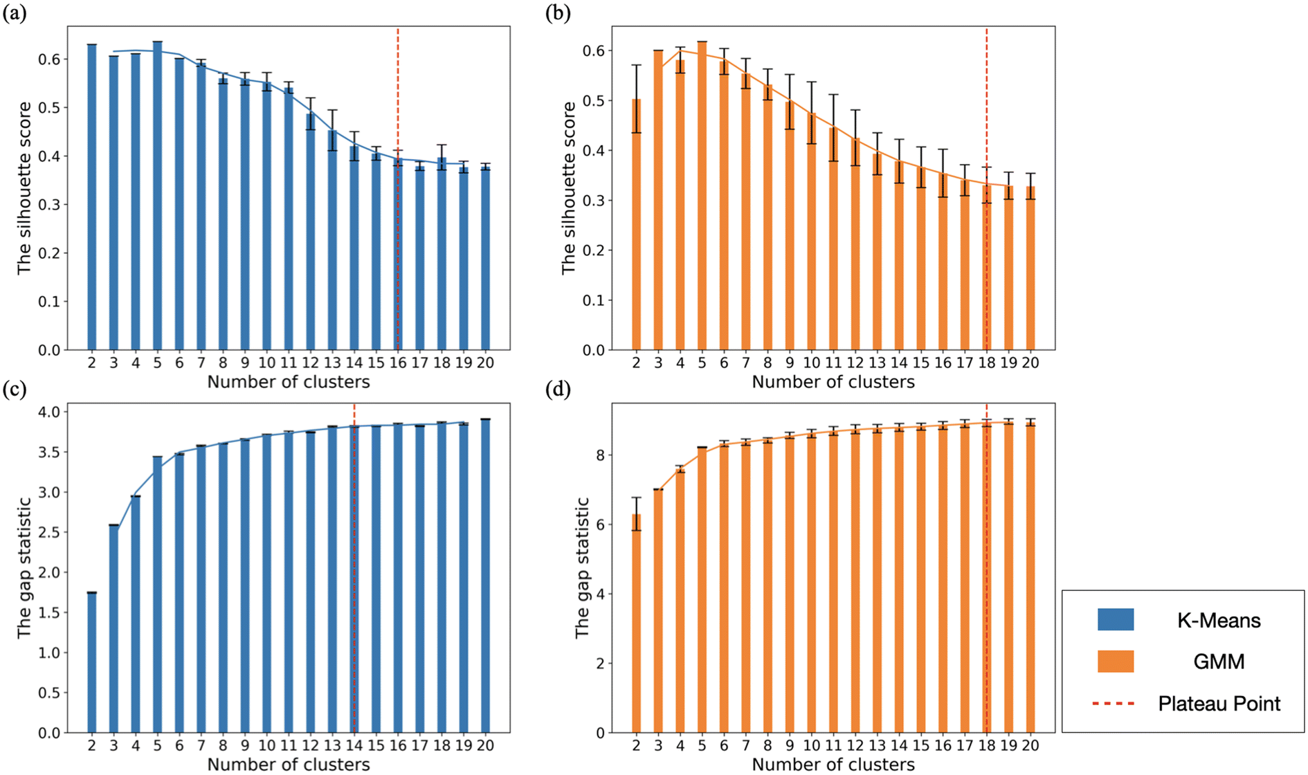

Fig. 4 Evaluation of clustering performance using the silhouette score and gap statistic for the Ag dataset with clusters ranging in size from 2 to 20. (a) Silhouette score for K−means clustering. (b) Silhouette score for GMM clustering. (c) Gap statistic for K−means clustering. (d) Gap statistic for GMM clustering. The dashed red line indicates the plateau point for each method, representing the optimal number of clusters based on the respective evaluation metric. Error bars denote the standard deviation obtained from multiple runs.

We observed plateau values in the silhouette score at N = 16 and 18 for the PCA + K−means [Fig. 4(a)] and PCA + GMM [Fig. 4(b)] methods, respectively. The gap statistic score calculated for the PCA + K−means [Fig. 4(c)] and the PCA + GMM [Fig. 4(d)] methods reaches a plateau after N = 14 and 18, respectively. The elbow point in the gap statistic at N = 6 suggests that this number of clusters balances model complexity and within-cluster variance well, but the larger gap statistic scores at N = 14 and 18 indicate that 14 and 18 clusters still provide a better fit than 6 clusters in terms of reducing within-cluster variance. Given the statistical results, using 14 to 18 clusters appears to be a reasonable and justified decision. By characterizing the detailed structures of nanoparticles within each cluster using CNA analysis, we determined that the K−means method best distinguished between 14 structural classes for this dataset, with at least five data points in each class and the fewest mis-classifications. These classes are indicated in Fig. 5.

Fig. 5 Representative Ag structures for clustering into 5 and 14 groups, using PCA + K−means. The inner pie chart shows the 5 major clusters: FCC/SCSF, Dh, Dh–Ih, Ih, and amorphous. The outer pie chart shows the 14 sub-clusters within the 5 major clusters. Distinguishing features of each cluster are shown: turquoise atoms show bulk features, yellow atoms show surface features, and the red atoms are Ih centers.

The first three classes in Fig. 5 pertain to FCC and SCSF structures: class 1 contains single-crystal structures (FCC) across the entire size range. Class 2 and class 3 each contain SCSF structures with one layer of stacking fault and multiple layers of stacking faults, respectively. Each of these two classes contain SCSF for almost the entire size range. Class 4 consists of Dh with different lengths of the five icosahedral surface edges, while class 5 consists of Dh with five icosahedral surface edges of identical lengths. These two classes also include nanoparticles across the entire size range.

The next four classes pertain to various types of Dh–Ih nanocrystals. The major difference between them is the percentage of unclassified atoms. Class 6, 7, 8 and 9 each consists of Dh–Ih with less than 10%, 10–20%, 20–25%, and 25–30% of unclassified atoms, respectively. Here, we note that 116 atoms is a magic size for a Dh–Ih.⁴⁷ Class 6 contains Dh–Ih nanocrystals close to this magic size, consisting of perfect Ag₁₁₆ Dh–Ih structures with both missing and extra surface atoms, ranging from Ag₁₁₄ to Ag₁₁₇. This is the only class of Dh–Ih structures observed over a small size range.

There are three classes for Ih structures. Class 10 contains Ih with less than 7% of atoms from the Ih/Dh notch vertex environment and more than 23% of atoms from Ih surface edge environment. Class 11 is the only Ih class containing structures with more than 20% of atoms from the HCP bulk environment. It is also the only Ih class containing structures with 140 atoms, close to the magic size of a perfect Ih with 147 atoms. Class 12 contains Ih with 7–20% of atoms from the Ih/Dh notch vertex environment and less than 23% of atoms from Ih surface edge environment. Class 13 and 14 are amorphous structures with different proportions of ordered atoms (30–40% for class 13 and less than 30% for class 14). Representative structures for each cluster are shown in Fig. 5.

Fig. 6 illustrates the fraction of each relevant CNA environment for each of the FCC/SCSF nanocrystals in classes 1–3 in Fig. 5. Here, we see a distinct CNA grouping for each class, with no HCP atoms in class 1, and an increasing fraction of HCP atoms in going from class 2 to class 3 – consistent with an increasing number of stacking faults. We also see an increasing cumulative fraction of “other” atoms, that contribute less than 5% each to the total, as we go from class 1 to class 3. We show a similar CNA breakdown for the other classes for Ag in the ESI, in Fig. S1–S4.†

Fig. 6 Fraction of atomic CNA environments (see Table 1) for the three FCC/SCSF classes in Fig. 5. The category labeled “others” contains the sum of fractions of individual CNA environments that contribute less than 5% to the total.

Telari et al. used convolutional neural networks based on radial distribution functions to classify the structures of Ag nanoparticles containing 147 atoms, generated with PTMD.⁴⁰ Their description of Ag interactions was given by the Gupta potential,⁵⁹ which is different than the EAM potential that we used for the structures in this study. Overall, they distinguished five broad classes for these structures, with 17 different fine classes. Similar to us, their broad classes contained Ih, FCC/SCSF, Dh-like and amorphous structures. However, they introduced a different class denoted “distorted” and it is unclear whether this class has good agreement with our Dh–Ih class.

Their fine structural classes contained four types of Ih, while we found three types – however, they probed a magic size for an Ih in their study, so finding four Ih is perhaps not surprising. Similar to us, they found three different classes of FCC/SCSF. They found a single Dh-like class, while we found two Dh classes. However, they identified seven different classes of amorphous nanoparticles (to our two) and two “distorted” structures. In addition to differences between the ML methods and interatomic potentials employed, they studied only Ag₁₄₇, while we probed an entire size range. We also note that the results in Fig. 4 indicate that N = 14–18 is an adequate size range for classifying the nanoparticle structures in our study and when we use N > 15, the “extra” structures are classified as amorphous.

Roncaglia and Ferrando also studied Ag₁₄₇ nanoparticles using ML methods similar to ours.³⁸ They generated their nanoparticle structures using a combination of optimization and MD simulations run at temperatures around the solid–liquid transition. Similar to Telari et al., they used the Gupta potential to describe Ag interactions. They found that three PCs captured more than 99% of their variance (we found four captured greater than 95%) and they identified 14 different structural classes. Most of the structures they identified were Ih-like, which is perhaps not surprising, given that 147 atoms is a magic size for an Ih. However, Telari et al. also studied Ag₁₄₇ based on the Gupta potential and their ML classification contained a broad range of structures comparable to the range that we identified by studying different nanoparticle sizes. These differences highlight the importance of the ML method and perhaps also the method for structural generation in establishing a comprehensive shape classification.

3.4 Cu shape categories

Fig. 7 shows the silhouette score [Fig. 7(a) and7(b)] and gap statistic [Fig. 7(c) and (d)] for both K−means and GMM clustering of Cu. For Cu, the largest silhouette score was found at N = 2 for both K−means and GMM clustering, but this oversimplifies the structure in the data by only separating the data points into crystalline and amorphous structures. The silhouette score and gap statistic both exhibit a plateau at N = 5, showing the same shape classes as we see for Ag: FCC/SCSF, Dh, Dh–Ih, Ih, and amorphous. By analyzing the CNA signatures from each cluster for N = 6, we found that FCC and SCSF become distinct classes, with the rest of the classes the same as for N = 5.

Fig. 7 Evaluation of clustering performance using silhouette score and gap statistic for the Cu dataset for clusters ranging in size from 2 to 20. (a) Silhouette score for K−means clustering. (b) Silhouette score for GMM clustering. (c) Gap statistic for K−means clustering. (d) Gap statistic for GMM clustering. The dashed red line indicates the plateau point for each method, as described in the text. Error bars denote the standard deviation obtained from multiple runs.

The gap statistic calculated for the PCA + K−means and PCA + GMM methods reaches a plateau after N = 17 and 18, respectively. We also observed that the silhouette score plateaued at N = 15 and 16 for the PCA + K−means and PCA + GMM methods, respectively. By analyzing the detailed CNA signatures within each cluster, we determined that the K−means method best distinguished between 15 structural classes for this dataset. These 15 clusters are more detailed sub-clusters within the 5 major clusters described above.

Fig. 8 shows the hierarchy of structural classes observed for the Cu nanoparticles. At the most basic level, unsupervised learning distinguishes between crystalline and amorphous nanoparticles (N = 2). It is interesting that this clustering was not seen for Ag – though the silhouette score for K−means clustering with N = 2 has the second-highest value for Ag. Similar to Ag, we find five different structural classes for Cu, with 15 detailed classes within the five major classes. Fig. S5–S9† show the CNA signatures for each structure in each of the five classes, along with their delineation into the 15 sub-classes.

Fig. 8 Representative Cu structures for clustering into 2, 5, and 15 groups, using PCA + K−means. The innermost pie chart shows two basic structural features: crystalline and amorphous. The middle pie chart shows the 5 major clusters: FCC/SCSF, Dh, Dh–Ih, Ih, and amorphous. The outer pie chart shows the 15 sub-clusters within the five major clusters. Distinguishing features of each cluster are shown: turquoise atoms show bulk features, yellow atoms show surface features, and the red atoms are Ih centers.

Delving into the fine structural classes, the first two classes pertain to FCC structures: class 1 consists of pure FCC single crystal structures and SCSF structures with one stacking-fault, while class 2 consists of SCSF structures with multiple stacking faults. It appears the delineation between FCC and SCSF structures is more distinct for Ag than for Cu.

Classes 3 and 4 deal with Dh structures: Dh structures in class 3 possess less than 1% of atoms from the Ih/Dh surface vertex environment, while Dh structures in class 4 have 1–2% of atoms from the Ih/Dh surface vertex environment. Neither of these classes is restricted to a specific size range.

Classes 5–8 pertain to various types of Dh–Ih structures. Class 5 consists of Dh–Ih structures with two half-sets of perfect Ih-spine, ranging in size from 180–200 atoms. Classes 6, 7, and 8 contain Dh–Ih nanocrystals close to the magic size at 116 atoms,⁴⁷ but each having its own characteristic atomic environment. Dh–Ih nanocrystals from class 6 possess a perfect five-fold ring formed by Ih spine atoms, while Dh–Ih nanocrystals from class 7 also have the five-fold ring-like structure but with missing atoms. Dh–Ih structures from class 8 have a linear Ih spine, similar to a Dh.

There are four classes for Ih structures. Class 9 is the only Ih class containing structures with a complete set of perfect Ih spines, with a number of atoms ranging from 150 to 160. Classes 10 and 11 contain Ih structures across the entire size range. The major difference between these classes is that the percentage of atoms from the Ih/Dh notch vertex environment is greater than 5% and smaller than 10% in class 10, while it is smaller than 5% in class 11. Class 12 contains Ih nanocrystals similar to a “twisted”, anti-Mackay Ih with 116 atoms,⁴⁸ with both extra and missing surface atoms. Classes 13, 14, and 15 are amorphous structures with different proportions of ordered atoms (10–20% for class 13, 20–30% for class 14, and 30–40% for class 15).

Telari et al. used convolutional neural networks based on radial distribution functions to classify the structures of Cu nanoparticles containing 147 atoms, generated with PTMD based on the Gupta potential. Overall, they distinguished six broad classes for these structures, with 22 different finer classes. Similar to us, their broad classes contained Ih, FCC/SCSF, Dh-like, and amorphous structures. However, they found a class consisting of pure HCP structures and introduced a different class denoted “intermediate”, which may correspond to the Dh–Ih structure that we find here.

Their fine structural classes contained seven types of Ih, while we found four types. This may reflect that their study was conducted at a magic size for an Ih. They found four different classes of FCC/SCSF, while we found two. In both our study and theirs, two Dh classes were identified. They identified six different classes of amorphous nanoparticles, while we found three. They also found one HCP class, which we did not observe, and two “intermediate” structures, which may correspond to our Dh–Ih. It seems possible that some of the differences between our studies arise from the sizes probed in their study (Cu₁₄₇) vs. ours (Cu₁₀₀–Cu₂₀₀), as well as from differences in the potentials used and ML methods in the two studies.

Overall, comparing our shape classifications for Ag and Cu nanocrystals, we see that FCC and SCSF shapes tend to be more emphasized for Ag and Ih shapes tend to be more prominent for Cu. This is consistent with PTMD results for the two systems,^47,48 which employed just the five inner/middle shapes classes in Fig. 5 and 8. Doye, Wales, and Berry studied the effect of the energetically preferred shape of a cluster on the range of the inter-atomic pair potential (a Morse potential) and the size of the cluster.⁶⁰ For sufficiently large clusters in their study (an admittedly small size range of 25–80 atoms), they found that the structure of the global minimum changed from Ih to Dh to FCC as the range of the potential was decreased. The argument is that strain (that is found in Ih structures but not in FCC) is better accommodated in a long-ranged potential than in a short-ranged one. We note that the cut-off distance is greater for the EAM potential for Cu⁶¹ than it is for Ag,⁵¹ even though the lattice constant is larger for Ag. These observed differences between Ag and Cu await experimental confirmation.

4 Conclusions

In this study, we applied unsupervised learning techniques, including PCA for dimensionality reduction, as well as K−means and GMM clustering to classify monometallic Ag and Cu nanoparticles based on CNA features. We found that K−means provides a more suitable clustering of the data in our study than GMM. For Ag, we found five structural classes, with 14 detailed sub-classes, while for Cu, we found two broad classes (crystalline and amorphous), with the same five classes as for Ag, and 15 detailed sub-classes. Our results demonstrate that these ML methods are effective in identifying and categorizing nanoparticle structures to different levels of complexity, enabling us to classify nanoparticles into distinct and physically meaningful structural classes with high accuracy. This capability is crucial for understanding nanoparticle properties and potential applications.

The methodology we use here could be easily extended to larger systems with appropriate adjustments. For larger nanoparticles, it is possible that additional structural motifs could emerge, and the complexity of the nanoparticle shapes might increase. To adapt our methodology for larger systems, the feature set would need to be expanded to include new CNA signatures that account for these additional motifs. Similarly, these studies could be extended to bimetallic systems using adaptive CNA.⁶² Since CNA only depends on the capability to define a set of atomic coordinates (and identities, in the case of multi-metallic nanocrystals), such techniques could be applied to experimental data. In all cases, the computational requirements of the ML methods are relatively modest, and these calculations can be performed on a laptop or a desktop computer.

We obtained different classification results than those in prior studies of Ag and Cu,^38,40 which could be due to the wider size range probed in our study, as well as the different atomic potentials – EAM in our study vs. Gupta in theirs. However, the studies of Roncaglia³⁸ and Telari⁴⁰ probed Ag nanocrystals of the same size and with the same inter-atomic potential, but different ML methods, and they achieved significantly different classification results.

The differences between all our results highlight the need for consistent nomenclature in categorizing nanocrystals and the need to better evaluate the ML methods employed. Since differences between our results and those of Roncaglia and Telari may indicate a sensitivity to the atomic potential, there is room for the application of more accurate atomic potentials with higher fidelity to first principles, such as ML force fields. Differences between these three studies may also indicate that structural classification with ML methods is highly sensitive to the ways in which structures are generated. Differences in structural generation could explain the differences between the study of Roncaglia³⁸ and Telari⁴⁰ and why the structures in our study are similar to those found by Telari et al. This indicates the possibility that ML methods can link fine structural details to materials processing methods. The methods applied here could conceivably be applied in experiments, which would allow for detailed testing of the level of theory that needs to be applied to describe nanocrystals accurately. Further research in this direction would be fruitful.

Data availability

The coordinates of the Ag and Cu nanocrystals in this article are available in the ESI of ref. 47 and 48, respectively. In the ESI,† we provide files containing the 207 and 176 data points we used for Ag and Cu, respectively. Each row in the file represents a distinct nanoparticle structure, each column represents a CNA signature we used as a feature, and each number represents a percentage of the atoms from each atomic environment.

Conflicts of interest

There are no conflicts to declare.

Acknowledgements

This work was funded by the Department of Energy, Office of Basic Energy Sciences, Materials Science Division, grant DE-FG02-07ER46414. This work used Bridges-2 at the Pittsburgh Supercomputing Center through allocation DMR110061 from the Advanced Cyberinfrastructure Coordination Ecosystem: Services & Support (ACCESS) program, which is supported by National Science Foundation grants #2138259, #2138286, #2138307, #2137603, and #2138296.

References

1. J. Li, C. Zhang, Y. Li, Y. Pan and Y. Liu, ACS Catal., 2023, 13, 9633–9655.
2. K. Zhang, C. Wang, F. Gao, S. Guo, Y. Zhang, X. Wang, S. Hata, Y. Shiraishi and Y. Du, Coord. Chem. Rev., 2022, 472, 214775.
3. B. S. Goo, K. Ham, Y. Han, S. Lee, H. Jung, Y. Kwon, Y. Kim, J. W. Hong and S. W. Han, Angew. Chem., Int. Ed., 2022, 61, e202202923.
4. J. Ma, X. Tan, Q. Zhang, Y. Wang, J. Zhang and L. Wang, ACS Catal., 2021, 11, 3352–3360.
5. J. Zhang and W. Wu, Plasmonics, 2024, 1–9.
6. P. Cheng, Y. An, A. K. Jen and D. Lei, Adv. Mater., 2023, e2309459.
7. V. Coviello, D. Forrer and V. Amendola, ChemPhysChem, 2022, 23, e202200136.
8. Y. Lin, T. Fang, C. Bai, Y. Sun, C. Yang, G. Hu, H. Guo, W. Qiu, W. Huang, L. Wang, Z. Tao, Y. Q. Lu and D. Kong, Nano Lett., 2023, 23, 11174–11183.
9. Y. Guan, F. Xu, L. Sun, Y. Luo, R. Cheng, Y. Zou, L. Liao and Z. Cao, Sensors, 2023, 23, 8536.
10. L. Cheng, D. Ruan, Y. He, J. Yang, W. Qian, L. Zhu, P. Zhu, H. Wu and A. Liu, J. Mater. Chem. C, 2023, 11, 8413–8422.
11. P. K. Kalambate, J. Noiphung, N. Rodthongkum, N. Larpant, P. Thirabowonkitphithan, T. Rojanarata, M. Hasan, Y. H. Huang and W. Laiwattanapaisal, Trends Anal. Chem., 2021, 143, 116403.
12. G. Zeng, W. Chen, X. Chen, Y. Hu, Y. Chen, B. Zhang, H. Chen, W. Sun, Y. Shen, Y. Li, F. Yan and Y. Li, J. Am. Chem. Soc., 2022, 144, 8658–8668.
13. S. K. Hazra, A. M. Saleque, A. K. Thakur, M. N. A. S. Ivan, D. Biswas, S. A. Khan, R. Saidur, Z. Ma and R. Sathyamurthy, Energy Technol., 2024, 12, 2301190.
14. Z. Li, X. Xu, X. Sheng, P. Lin, J. Tang, L. Pan, Y. V. Kaneti, T. Yang and Y. Yamauchi, ACS Nano, 2021, 15, 12535–12566.
15. C. M. Sheng, N. Yang, Y. T. Yan, X. P. Shen, C. D. Jin, Z. Wang and Q. F. Sun, Appl. Therm. Eng., 2020, 167, 114712.
16. X. Wang, T. Y. Li, W. H. Geng, Z. Bao, P. F. Qian, L. C. Jing, P. S. Bin, Z. X. Yang, X. L. Liu and H. Z. Geng, ACS Appl. Mater. Interfaces, 2023, 15, 22762–22776.
17. N. N. Zhou, H. R. Ao, X. M. Chen and H. Y. Jiang, Nano Energy, 2022, 96, 107127.
18. F. Qin, Z. Y. Yan, J. F. Fan, J. L. Cai, X. Z. Zhu and X. G. Zhang, Macromol. Mater. Eng., 2021, 306, 2000607.
19. W. Zhang, H. Z. Li and A. Y. Elezzabi, Adv. Mater. Interfaces, 2022, 9, 2200021.
20. J. L. Wang, S. Z. Sheng, Z. He, R. Wang, Z. Pan, H. Y. Zhao, J. W. Liu and S. H. Yu, Nano Lett., 2021, 21, 9976–9982.
21. C. Eyovge, C. S. Deenen, F. Ruiz-Zepeda, S. Bartling, Y. Smirnov, M. Morales-Masis, A. Susarrey-Arce and H. Gardeniers, ACS Appl. Nano Mater., 2021, 4, 8600–8610.
22. I. Ali, M. R. Islam, J. Yin, S. J. Eichhorn, J. Chen, N. Karim and S. Afroj, ACS Nano, 2024, 18, 3871–3915.
23. M. L. R. Liman, M. T. Islam and M. M. Hossain, Adv. Electron. Mater., 2022, 8, 2100578.
24. P. Won, J. J. Park, T. Lee, I. Ha, S. Han, M. Choi, J. Lee, S. Hong, K. J. Cho and S. H. Ko, Nano Lett., 2019, 19, 6087–6096.
25. C. Zhang, Y. Zhou and C. Ye, Nanotechnology, 2024, 35, 325502.
26. X. Yang, W. Chen, Q. Fan, J. Chen, Y. Chen, F. Lai and H. Liu, Adv. Mater., 2024, 2402542.
27. M. Iqbal, Y. V. Kaneti, J. Kim, B. Yuliarto, Y. M. Kang, Y. Bando, Y. Sugahara and Y. Yamauchi, Small, 2019, 15, e1804378.
28. C. Xiao, B. A. Lu, P. Xue, N. Tian, Z. Y. Zhou, X. Lin, W. F. Lin and S. G. Sun, Joule, 2020, 4, 2562–2598.
29. K. A. Fichthorn and T. Yan, J. Phys. Chem. C, 2021, 125, 3668–3679.
30. K. A. Fichthorn, Chem. Rev., 2023, 123, 4146–4183.
31. M. Fernandez and A. S. Barnard, ACS Nano, 2015, 9, 11980–11992.
32. B. Sun, H. Barron, G. Opletal and A. S. Barnard, J. Phys. Chem. C, 2018, 122, 28085–28093.
33. T. Yan, B. Sun and A. S. Barnard, Nanoscale, 2018, 10, 21818–21826.
34. A. J. Parker, G. Opletal and A. S. Barnard, J. Appl. Phys., 2020, 128, 14301.
35. A. S. Barnard and G. Opletal, Nano Futures, 2020, 4, 035003.
36. Z. J. Zhao, S. H. Liu, S. J. Zha, D. F. Cheng, F. Studt, G. Henkelman and J. L. Gong, Nat. Rev. Mater., 2019, 4, 792–804.
37. S. C. Li and A. S. Barnard, Adv. Theory Simul., 2022, 5, 2100414.
38. C. Roncaglia and R. Ferrando, J. Chem. Inf. Model., 2023, 63, 459–473.
39. C. Roncaglia, D. Rapetti and R. Ferrando, Phys. Chem. Chem. Phys., 2021, 23, 23325–23335.
40. E. Telari, A. Tinti, M. Settem, L. Maragliano, R. Ferrando and A. Giacomello, ACS Nano, 2023, 17, 21287–21296.
41. X. Wang, J. Li, H. D. Ha, J. C. Dahl, J. C. Ondry, I. Moreno-Hernandez, T. Head-Gordon and A. P. Alivisatos, JACS Au, 2021, 1, 316–327.
42. H. Wen, J. M. Luna-Romera, J. C. Riquelme, C. Dwyer and S. L. Y. Chang, Nanomaterials, 2021, 11, 2706.
43. M. Botifoll, I. Pinto-Huguet and J. Arbiol, Nanoscale Horiz., 2022, 7, 1427–1477.
44. I. A. Moreno-Hernandez, M. F. Crook, V. Jamali and A. P. Alivisatos, MRS Bull., 2022, 47, 305–313.
45. E. M. Williamson, A. M. Ghrist, L. R. Karadaghi, S. R. Smock, G. Barim and R. L. Brutchey, Nanoscale, 2022, 14, 15327–15339.
46. N. Gumbiowski, K. Loza, M. Heggen and M. Epple, Nanoscale Adv., 2023, 5, 2318–2326.
47. T. Yan, H. Zhang and K. A. Fichthorn, ACS Nano, 2023, 17, 19288–19304.
48. H. Zhang, M. A. Khan, T. Yan and K. A. Fichthorn, Nanoscale, 2024, 11146–11155.
49. Y. Sugita and Y. Okamoto, Chem. Phys. Lett., 1999, 314, 141–151.
50. D. J. Earl and M. W. Deem, Phys. Chem. Chem. Phys., 2005, 7, 3910–3916.
51. P. L. Williams, Y. Mishin and J. C. Hamilton, Modell. Simul. Mater. Sci. Eng., 2006, 14, 817.
52. C. L. Cleveland, W. D. Luedtke and U. Landman, Phys. Rev. B: Condens. Matter Mater. Phys., 1999, 60, 5065–5077.
53. F. Pedregosa, G. Varoquaux, A. Gramfort, V. Michel, B. Thirion, O. Grisel, M. Blondel, P. Prettenhofer, R. Weiss and V. Dubourg, et al. , J. Mach. Learn. Res., 2011, 12, 2825–2830.
54. K. Pearson, The London, Edinburgh, and Dublin Philosophical Magazine and Journal of Science, 1901, vol. 2, pp. 559–572.
55. S. Lloyd, IEEE Trans. Inf. Theory, 1982, 28, 129–137.
56. C. M. Bishop, Springer Google Scholar, 2006, vol. 2, pp. 5–43.
57. P. J. Rousseeuw, J. Comput. Appl. Math., 1987, 20, 53–65.
58. R. Tibshirani, G. Walther and T. Hastie, J. R. Stat. Soc., Ser. B: Stat. Methodol., 2001, 63, 411–423.
59. R. P. Gupta, Phys. Rev. B: Condens. Matter Mater. Phys., 1981, 23, 6265–6270.
60. J. P. K. Doye, D. J. Wales and R. S. Berry, J. Chem. Phys., 1995, 103, 4234–4249.
61. Y. Mishin, M. J. Mehl, D. A. Papaconstantopoulos, A. F. Voter and J. D. Kress, Phys. Rev. B: Condens. Matter Mater. Phys., 2001, 63, 224106.
62. A. Stukowski, Modell. Simul. Mater. Sci. Eng., 2012, 20, 045021.

---

Footnote

† Electronic supplementary information (ESI) available: CNA signatures used in this study; detailed CNA analysis of all the structures in this study; input for machine learning for all the Cu and Ag nanoparticles. See DOI: https://doi.org/10.1039/d4nr02531h

---