
 Open Access Article
 This Open Access Article is licensed under a
 Creative Commons Attribution 3.0 Unported Licence
Experimental and simulation study of self-assembly and adsorption of glycerol monooleate in n-dodecane with varying water content onto iron oxide†
Alexander J.
Armstrong
 ab,
Rui F. G.
Apóstolo
cd,
Thomas M.
McCoy
b,
Finian J.
Allen
a,
James
Doutch
a,
Beatrice N.
Cattoz
e,
Peter J.
Dowding
e,
Rebecca J. L.
Welbourn
a,
Alexander F.
Routh
b and
Philip J.
Camp
*d
ab,
Rui F. G.
Apóstolo
cd,
Thomas M.
McCoy
b,
Finian J.
Allen
a,
James
Doutch
a,
Beatrice N.
Cattoz
e,
Peter J.
Dowding
e,
Rebecca J. L.
Welbourn
a,
Alexander F.
Routh
b and
Philip J.
Camp
*d
aISIS Neutron and Muon Source, Didcot, UK
bInstitute for Energy & Environmental Flows and Department of Chemical Engineering and Biotechnology, University of Cambridge, Cambridge, UK
cEPCC, Bayes Centre, 47 Potterrow, Edinburgh EH8 9BT, Scotland, UK
dSchool of Chemistry, University of Edinburgh, David Brewster Road, Edinburgh EH9 3FJ, Scotland, UK. E-mail: philip.camp@ed.ac.uk; Tel: +44 (0)131 650 4763
eInfineum UK Ltd, Milton Hill, UK
First published on 21st December 2023
Abstract
The self-assembly and surface adsorption of glycerol monooleate (GMO) in n-dodecane are studied using a combination of experimental and molecular dynamics simulation techniques. The self-assembly of GMO to form reverse micelles, with and without added water, is studied using small-angle neutron scattering and simulations. A large-scale simulation is also used to investigate the self-assembly kinetics. GMO adsorption onto iron oxide is studied using depletion isotherms, neutron reflectometry, and simulations. The adsorbed amounts of GMO, and any added water, are determined experimentally, and the structures of the adsorbed films are investigated using reflectometry. Detailed fitting and analysis of the reflectometry measurements are presented, taking into account various factors such as surface roughness, and the presence of impurities. The reflectometry measurements are complemented by molecular dynamics simulations, and good consistency between both approaches is demonstrated by direct comparison of measured and simulated reflectivity and scattering length density profiles. The results of this analysis are that in dry systems, GMO adsorbs as self-assembled reverse micelles with some molecules adsorbing directly to the surface through the polar head groups, while in wet systems, the GMO is adsorbed onto a thin layer of water. Only at high surface coverage is some water trapped inside a reverse-micelle structure; at lower surface coverages, the GMO molecules associate primarily with the water layer, rather than self-assemble.
1 Introduction
The adsorption of molecules at the solid–liquid interface underpins a vast range of chemical and engineering processes, including colloidal stabilisation, friction modification, lubrication, sensing, and surface passivation. The binding of molecules to a solid substrate, their organisation into a monolayer or multilayer structure, and the response of the adsorbed film to chemical and mechanical perturbations result in a modification of the solid–liquid interface, and its structural and dynamical properties. In the context of lubrication, it was shown in the 1920s that the adsorption of fatty acids to form a monolayer at metal–oil interfaces was sufficient to reduce friction and improve lubrication.1–3 Many similar molecules, with polar head groups and unsaturated tails, have proven to be effective organic friction modifiers in engines and motors. The adsorbed-film structures of such molecules on inorganic surfaces in hydrocarbons have been examined using a wide range of contemporary techniques, including sum-frequency generation spectroscopy, and (polarised) neutron reflectometry (NR).4–7 These methods yield information on the binding of the adsorbate to the surface, the surface coverage, the film thickness, and the molecular orientation with respect to the surface.In solution, surfactant-like molecules can also self-assemble to form structures such as micelles and reverse micelles (RMs). RMs formed by amphiphilic molecules in hydrocarbon solvents are well known.8–15 Small amounts of water are sometimes needed to promote full RM formation, and this water becomes localised in the micelle core.16,17 The surfactant of interest in the current work is glycerol monooleate (GMO), a non-toxic organic friction modifier, the structure of which is shown in Fig. 1. GMO forms RMs in aliphatic hydrocarbons,12 shown using small-angle X-ray scattering (SAXS), and a variety of self-assembled micelles and liquid-crystalline phases in water,18 shown with a combination of NMR spectroscopy, polarising optical microscopy, SAXS, and rheological measurements. The self-assembly of GMO in hydrocarbons (n-hexane or toluene) was also studied using a combination of small-angle neutron scattering (SANS) and molecular-dynamics (MD) simulations.19 A quantitative comparison was made between experimental and simulated form factors, which showed that the micelle radius of gyration was around 15 Å, and the aggregation number was in the region of 20–30, depending on the solvent. The radii of gyration determined from simulation and experiment were in agreement, with values within approximately 1 Å. This gives confidence on the fidelity of the molecular-scale structures generated using MD simulations, and in particular, the spatial distributions of GMO, solvent, and any ‘impurity’ (such as water) within the RM structure. Subsequent simulation work was carried out to study the adsorption of GMO RMs at the mica–hydrocarbon interface,20 and it was shown that there is a competition between self-assembly and adsorption, resulting in micelle-like structures persisting at the inorganic surface. This has not yet been confirmed experimentally.
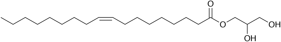 | ||
| Fig. 1 The molecular structure of glycerol monooleate [CH3(CH2)7CHCH(CH2)7COOCH2CHOHCH2OH]. | ||
In recent experimental work, a cell has been developed that allows the interfacial structures of adsorbed films to be studied under shear conditions using either X-ray or neutron reflectometry.21 In the initial demonstration of the cell, GMO was studied at the interface between n-dodecane and planar iron oxide (hematite, Fe2O3) surfaces. It was found that GMO forms a layer approximately 25 Å thick, which does not alter significantly between quiescent and shear conditions (shear rate 700 s−1). What has not yet been done in the case of GMO is to compare directly the results from reflectometry and MD simulations, and to investigate to what extent adsorbed-micelle structures can be resolved from the experiments. This is the objective of the current work.
Herein, a detailed comparison is made between experiments and MD simulations of GMO in n-dodecane (referred to as dodecane throughout the following sections) in bulk solution and at the interface with iron oxide. SANS is used to demonstrate that GMO forms well-defined RMs in bulk dodecane with and without added water (molar ratio 5![[thin space (1/6-em)]](https://www.rsc.org/images/entities/char_2009.gif) :1 H2O:GMO). A comparison is made between the experimental data and results from atomistic MD simulations of single RMs. The kinetics of RM formation with water are explored with a MD simulation containing 2 million atoms (including GMO, water, and dodecane). In the latter case, the system is so large that, on the simulation time scale of 51 ns, the spontaneous assembly of around 50 well-defined RMs is observed. The adsorption of GMO, with and without added water, onto iron oxide from dodecane is studied by measuring the adsorption isotherm, and by analysing the neutron reflectivity. These experiments give details on the amount of adsorbed material and some structural information on the adsorbed film, including its thickness. However, atomistic detail is not achievable with this approach. Therefore, MD simulations are carried out with the apparent amounts of adsorbed material, and the corresponding reflectivity profiles are computed from the simulated atomic density profiles. It is shown that it is possible to get almost perfect matches between simulations and experiments, which shows that the simulated structures are at least compatible with the available experimental data. Overall, it is shown that without water, GMO adsorbs onto iron oxide from dodecane as RMs, while with added water, it binds instead to a water film preferentially adsorbed to the iron oxide.
:1 H2O:GMO). A comparison is made between the experimental data and results from atomistic MD simulations of single RMs. The kinetics of RM formation with water are explored with a MD simulation containing 2 million atoms (including GMO, water, and dodecane). In the latter case, the system is so large that, on the simulation time scale of 51 ns, the spontaneous assembly of around 50 well-defined RMs is observed. The adsorption of GMO, with and without added water, onto iron oxide from dodecane is studied by measuring the adsorption isotherm, and by analysing the neutron reflectivity. These experiments give details on the amount of adsorbed material and some structural information on the adsorbed film, including its thickness. However, atomistic detail is not achievable with this approach. Therefore, MD simulations are carried out with the apparent amounts of adsorbed material, and the corresponding reflectivity profiles are computed from the simulated atomic density profiles. It is shown that it is possible to get almost perfect matches between simulations and experiments, which shows that the simulated structures are at least compatible with the available experimental data. Overall, it is shown that without water, GMO adsorbs onto iron oxide from dodecane as RMs, while with added water, it binds instead to a water film preferentially adsorbed to the iron oxide.
The rest of this article is organised as follows. Section 2 details the materials, SANS experiments, depletion-isotherm experiments, NR experiments, and MD simulations. Results are presented in Section 3, and are focused on self-assembly, adsorption, and the structures of adsorbed films. Section 4 concludes the article.
2 Methods
2.1 Materials
Glycerol monooleate (1-oleoyl-rac-glycerol, ≥99% purity) was purchased from Sigma Aldrich, UK, and stored below 0 °C. Hematite powder (α-Fe2O3) was purchased from Alfa Aesar (Puratronic, 99.995%). Dodecane-h26 was purchased from Fisher (≥99%, Acros Organics), and dodecane-d26 was purchased from Cambridge Isotope Laboratories (≥98% deuterated, 98% purity). Experiments were carried out with solutions of GMO in dodecane, both with and without added water. In the former case, the number of water molecules per GMO molecule (the hydration ratio) was ω = 5. Ultra-pure H2O dispensed from a purifier (Milli-Q IQ 7005) and D2O (99.9% deuterated, Sigma Aldrich) were used to dope the solutions of GMO dissolved in dodecane, which were then sonicated. When filling the SANS or reflectometry cells, aliquots were taken from the top of the wet samples to avoid including any non-solubilised water droplets that would coalesce at the bottom of the sample vials.For the NR measurements, silicon substrates with a quoted RMS roughness of 3 Å were purchased from Pi-Kem, UK, with l × w × h dimensions of either 55 mm × 55 mm × 10 mm (‘small substrate’) or 80 mm × 50 mm × 15 mm (‘large substrate’). Smooth iron oxide surfaces were provided by sputter coating the silicon substrates with iron, which was carried out by Pi-Kem.
2.2 Small-angle neutron scattering
SANS measurements were conducted on ZOOM at ISIS, UK. Samples were prepared using dodecane-d26 and analysed in 2 mm path length, quartz Hellma cuvettes that were positioned in an automated sample changer maintained at 25 °C. The instrument was configured with pinhole collimation, a source–sample detector distance set to 4 m, and a beam aperture of 8 mm × 8 mm. The resulting Q range was 0.004–0.7 Å−1, with the magnitude of the scattering vector, Q, being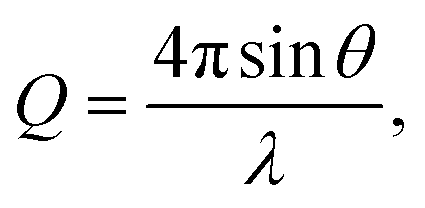 | (1) |
Modelling was performed using SasView V5.0.5 in combination with Bumps V0.9.023 to conduct Markov Chain Monte Carlo (MCMC) sampling using the DREAM algorithm. A spheroid form factor was parameterised (a reparameterisation of the ‘ellipsoid’ model within SasView), so that known characteristics of the system could be defined and constrained. Further details of the model are given in the ESI.† The parameter posterior distributions were all tested for normality with the D'Agostino–Pearson test,24,25 where the null hypothesis is that a given distribution is Gaussian. The parameters found to have p values greater than 1 × 10⁻³ are reported to be Gaussian with the subscript  in the notation
 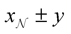 , where x and y are the mean and the symmetric 95% credible interval for a given Gaussian distribution.
2.3 Depletion isotherms
Solutions of GMO dissolved in dodecane-h26 were prepared at known concentrations before 0.5 g of powdered iron oxide was added to each solution and stirred for at least 5 hours. The solutions were stirred in a water bath to control the temperature throughout the experiment. The surface area of the iron oxide powder was found to be (11.8 ± 0.1) m2 g−1 by N2 BET sorption analysis carried out at the Department of Materials Science and Metallurgy, University of Cambridge, UK. The solutions were then left to stand for approximately 30 minutes in the water bath, allowing the majority of the powder to settle at the bottom. Approximately 7 mL of the liquid from the top of the sample was then removed and centrifuged at 10000 rpm. The supernatant was collected and the solutions were analysed via transmission Fourier transform infra-red (FTIR) spectroscopy using a PerkinElmer Spectrum 100 spectrometer equipped with a liquid N2-cooled mercury-cadmium-telluride detector. The remaining concentration of GMO within each sample was determined by integrating the IR adsorption in the region of 1665–1800 cm−1 arising from the ester carbonyl of GMO, followed by linear regression with a calibration data set from standards of known GMO concentrations.
2.4 Neutron reflectometry
NR was conducted on INTER at ISIS, UK.26 The range of the neutron wavelengths was 1.5–17.0 Å, and the scattering angles were 0.7°, 1.2°, and 2.3°. This resulted in a Q range of 0.009–0.331 Å−1. The illuminated length of the neutron beam footprint was approximately 40 mm and 60 mm for the small and large substrates, respectively. The resolution, δQ/Q, was constant over the Q range at approximately 2% and 3% for the small and large substrates, respectively.The substrates were cleaned with UV–ozone for 20 minutes before they were sealed within solid–liquid cells. Sample solutions were then passed into the cells prior to alignment of the solid–liquid interface with the neutron beam. The cells were equilibrated at 25 °C for 20 minutes before alignment, and were kept at these temperatures for the measurements. The reflected intensity was then collected for a minimum of 50 minutes over the three scattering angles, after which the data were normalised with transmission measurements, and then combined to form composite reflectivity profiles over the whole Q range using Mantid.22
Model selection was conducted by estimating the Bayesian evidence, Z, of candidate models for each reflectometry data set, as defined previously.27,28 This was achieved using the static nested sampling algorithm provided by the Python package dynesty V1.2.229 in combination with refnx V1.2930 to calculate the model reflectivity. The number of live points used in the nested sampling was 500, and the stopping criterion was the default of 0.509. Using the model with the greatest evidence, the posterior distribution for each parameter was estimated via MCMC sampling by using either the DREAM algorithm within Refl1d V0.8.1431 or the parallel-tempered affine invariant MCMC ensemble sampler (PT-MCMC) implemented as part of refnx. For all analyses, the data were modelled as evenly weighted linear combinations of the down-spin and up-spin reflectivities to account for the magnetic domain scattering on a non-polarised instrument. With this approach, it is assumed that the magnetic domains of the iron and iron oxide are larger than the neutron coherence length, and that there is no off-specular magnetic domain scatter. The parameter values reported in later sections are the median and 95% credible intervals (percentile). The parameter distributions were tested for normality via the aforementioned D'Agostino–Pearson test.
2.5 Molecular dynamics simulations
Classical MD simulations were performed using the LAMMPS software package,32–34 initial system configurations were created using Packmol,35 and the Visual Molecular Dynamics software was used for system visualisation and image rendering.36 The interactions involving GMO and solvent molecules were given by the all-atom, L-OPLS-AA force field,37–42 and cross interactions were evaluated using the Good–Hope43 and Berthelot
  mixing rules.44
2.6 Bulk-liquid simulations
Bulk-liquid simulations were carried out in cubic cells with periodic boundary conditions applied, Lennard-Jones interactions were cut at 12 Å, and long-range Coulomb interactions were handled using the particle–particle particle–mesh method with a relative accuracy in the forces of 1 × 10⁻⁴. In all cases, the systems were energy minimised, and then run under NPT conditions with T = 298.15 K and P = 1 atm using a Nosé–Hoover thermostat/barostat.45–48 The simulation time step was 1 fs, the thermostat damping time was 0.1 ps, and the barostat damping time was 1 ps.The self-assembly of single RMs was studied using, initially, 20 molecules of GMO in dry dodecane, and 30 molecules of GMO in dodecane with 150 molecules of water (ω = 5). 1400 molecules of dodecane were used in both cases. Each simulation was started from a uniform, randomly generated configuration in a cubic box with side 82 Å. The aggregation numbers were determined by a trial-and-error approach, where single molecules were deleted until the RM remained intact over the 20 ns simulation period. The radius of gyration, Rg, of an isolated RM was computed using a direct formula, and by fitting the corresponding form factor, P(Q). The direct formula is
 | (2) |
 | (3) |
Again, the interatomic distances were calculated with the periodic boundary conditions unwrapped.
There are several options for fitting the low-Q portion of P(Q) without assuming a specific shape of the self-assembled structures. First, there is the Guinier approximation
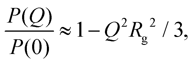 | (4) |
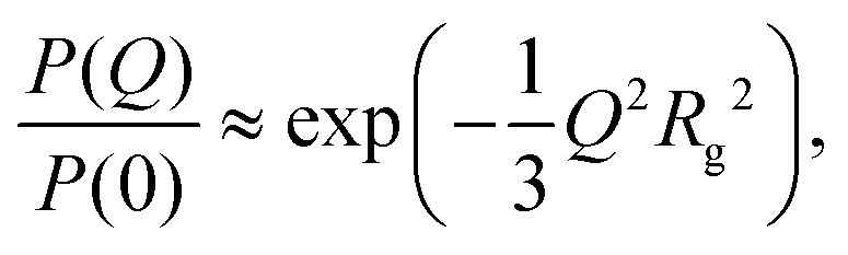 | (5) |
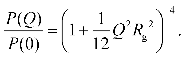 | (6) |
For uniform hard spheres with radius RHS, the form factor is
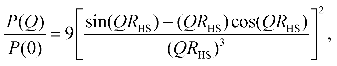 | (7) |
 . More complicated expressions apply for non-spherical objects, such as ellipsoids.
A large-scale simulation was also carried out to examine the formation kinetics of RMs, and to obtain another estimate of the equilibrium aggregation number. 1010 molecules of GMO, 5050 molecules of water (ω = 5), and 50500 molecules of dodecane were simulated in a cubic box of side 272 Å for 51 ns; this adds up to a total of 1999800 atoms, a GMO concentration of 83 mM, and a mass density of 747 kg m−3. This 51 ns simulation was run on ARCHER2, the UK National Supercomputing Service. The analysis of the results from this simulation is described in detail in Section 3.3.
2.7 Solid–liquid interface simulations
Simulations of surface-adsorbed GMO were carried out by confining the liquid between two parallel, planar iron oxide slabs with the (100) faces exposed. Hematite has a hexagonal unit cell with parameters a = b = 5.038 Å, c = 13.772 Å, α = β = 90°, and γ = 120°.49 Slabs were carved from the crystal structure and oriented in the laboratory frame (x, y, z) such that b‖y and c‖x; each slab had dimensions 55.088 Å × 50.38 Å × 8.61 Å, and contained 2400 atoms.The numbers of GMO molecules on each surface were determined from the NR experiments (see Sections 3.6 and 3.7). For a dry solution, full surface coverage equated to 78 GMO molecules per surface, and 156 molecules total. Half-coverage and quarter-coverage simulations were also carried out, with 78 and 39 GMO molecules total, respectively. For a wet solution, full surface coverage equated to 68 GMO molecules and 383 water molecules per surface for totals of 136 and 766, respectively, so that on the surface, ω = 5.6, which is higher than the bulk solution. This indicates preferential water adsorption, and as is shown in Section 3.8, the water forms a wetting layer on the iron oxide surface. Therefore, half-coverage and quarter-coverage simulations were carried out with 34 and 17 GMO molecules per surface, respectively, but the number of water molecules was kept fixed at 383.
The surface interactions were represented by the Lennard-Jones and Coulomb potentials determined by Berro et al.50 The specific values are given in Table S1 in the ESI,† along with a brief discussion of a recent new parameterisation against density functional theory calculations.51 Lennard-Jones interactions were cut at 12 Å, and the long-range Coulomb interactions were handled using a slab-adapted particle–particle particle–mesh method, designed to cancel out interactions between periodic images in the z direction,52 and with a relative precision in the forces of 1 × 10⁻⁴.
In each simulation, the system was energy minimised, thermostatted at T = 298.15 K, and allowed to equilibrate at constant volume. Then a constant-load simulation corresponding to a pressure of P = 1 atm was carried out by applying a constant, normal force to the outermost layer of atoms in the upper slab, while the outermost layer of atoms in the bottom slab was kept fixed.53 The system was simulated for 15 ns, and properties were computed from the last 5 ns of the trajectory.
3 Results and discussion
3.1 Self-assembly in solution: small-angle neutron scattering
Three solutions of GMO in dodecane-d26 (20 mM) were prepared, and two of them were doped with H2O or D2O (100 mM) so that the hydration ratio ω = 5. The two solutions doped with water are termed the wet systems, while the remaining solution is referred to as the dry system. The normalised scattering data collected with the dry and wet systems are shown in Fig. 2(a) and (b), where the difference between the contrasts collected with H2O and D2O arises from the difference in H and D content within the RMs due to the partitioning of water. The results are plotted on logarithmic scales rather than as functions of Q2 on linear scales because they are fitted with models that extend beyond the Guinier regime (4), and in addition, linearisation leads to biased estimates of the fitting parameters.54 Prior to fitting the data to the ellipsoid model, the data were fitted to the shape-independent Gaussian model (5) in the Q range of 0.004–0.081 Å−1 using SasView. The Rg values for the solutions doped with D2O and H2O were constrained to be the same. The resulting radii of gyration are shown in Table 1.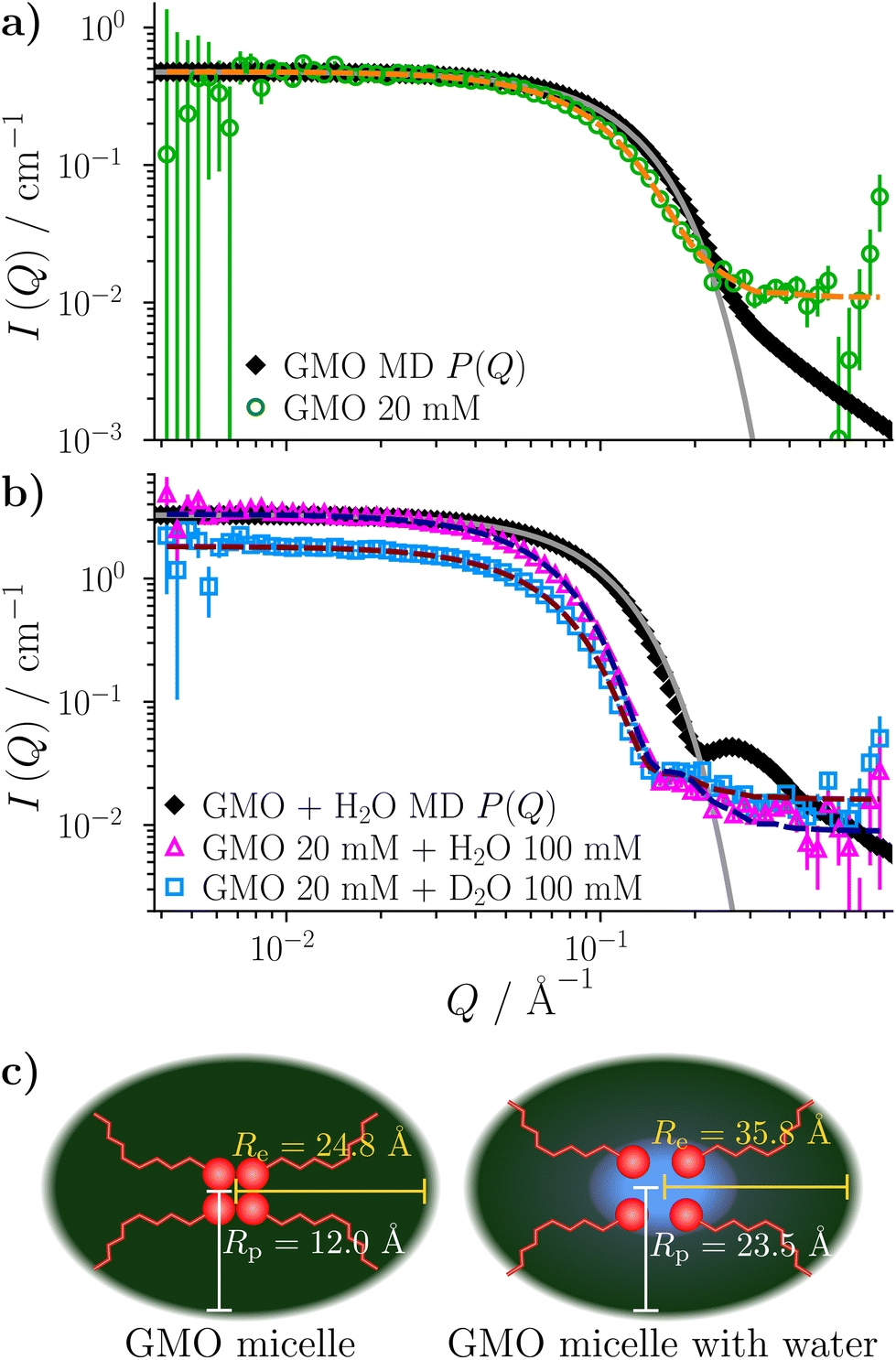 | ||
| Fig. 2 SANS profiles of 20 mM GMO in dodecane-d26 as (a) a ‘dry’ system and (b) with 100 mM of H2O or D2O added. The scatter data show the form factors of isolated RMs in both dry (ω = 0) and wet (ω = 5) conditions; the open points are from SANS experiments, and the filled points are from MD simulations. The MD form factors are scaled to match the fitted SANS scale factors for the dry system and the GMO + H2O system. The dashed lines show the model fit to each data set, while the full grey lines show the Gaussian model (5) fitted to the MD form factors (extended beyond the Q = 0.1 Å fit limit – see Table 2). (c) Schematic illustrating the ‘swelling’, depicted by changes in radii, of GMO RMs in dodecane following sequestration of water molecules into the reverse micelle interior. | ||
| System | R g/Å | R e/Å | R p/Å | R g,ellip/Å |
|---|---|---|---|---|
| Dry | 16.7 ± 0.5 | *16.1+0.3−0.2, †24.8 ± 0.5 | †12.0 ± 1.0, *30.4 ± 0.7 | 16.6+0.5−0.2 |
| Wet |
|
35.8 ± 0.2 | 23.5 ± 0.3 |
|
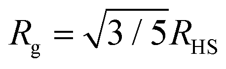
The ellipsoid model was then fitted to the data using the priors shown in Tables S2 and S3 in the ESI.† The dashed lines in Fig. 2(a) and (b) show the fitted scattering profiles. The parameter distributions are tabulated and visualised in Tables S4, S5, and Fig. S1, S2, in the ESI.† The eccentricity parameter for the dry system was found to be bimodal, where the mode with the greatest probability indicates that it is likely the RMs are oblate, although a prolate shape cannot be ruled out. The bimodal nature of the posterior distribution could reflect the fact that a unique fit is not achievable with a single contrast, rather than there being a bimodal distribution of RM sizes in solution. The equatorial and polar radii of the RMs, Re and Rp, were calculated from the fitted volume and eccentricity parameters for the dry and wet systems. The radius of gyration derived from the ellipsoid model is then55
 | (8) |
The derived radii are shown in Table 1, and the oblate RMs are depicted schematically in Fig. 2(c). The aggregation number (AN) for the dry system was calculated to be AN = NGMOV = 49.8+4.5−2.2, where NGMO and V are the number density of GMO and RM volume, respectively. The inclusion of water at ω = 5 swells the volume of the RMs by a factor of approximately four, which is thought to arise from absorption. The GMO aggregation number for the wet system was found to be  , where ϕGMO = 80.6% (fixed) is the volume fraction of GMO within the RMs.
Given that dodecane and water are essentially immiscible, the considerable uptake of water by the GMO RMs indicates highly favourable attractive interactions between the GMO head groups and water molecules. As previously mentioned, the swelling by a factor of four upon inclusion of water at ω = 5 is believed to be in part due to the added water promoting the formation of additional micelles (when compared to the dry system). This would further account for the increased scattering intensity at low Q with water present [Fig. 2(b)], and suggests a synergistic interplay underpinning GMO/water co-assembly.
3.2 Self-assembly in solution: MD simulation of a single reverse micelle
Simulations of single RMs were carried out, both in dry dodecane (ω = 0), and with five water molecules per GMO molecule (ω = 5). Using the trial-and-error approach, it was found that RMs with 18 and 28 GMO molecules remained intact over at least 20 ns. Final snapshots from each simulation are shown in Fig. 3.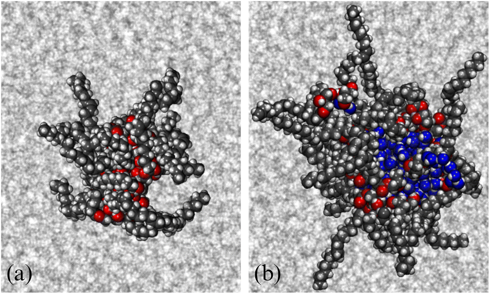 | ||
| Fig. 3 Molecular configurations at the end of 20 ns runs: (a) an RM of 18 GMO molecules in pure dodecane; (b) an RM of 28 GMO molecules and 150 water molecules, in dodecane. GMO atoms are shown in space-filling representation, while dodecane is shown in stick representation. GMO carbon atoms are shown in black, GMO oxygens in red, water oxygens in blue, hydrogens in white, and dodecane molecules in grey. | ||
The radii of gyration were computed directly (2), and by fitting various functions to the simulated form factor (3). The values of Rg from the fits are collected in Table 2. These show how the micelles grow in size with the inclusion of water, from Rg ≃ 14 Å at ω = 0 to Rg ≃ 17 Å at ω = 5. Nonetheless, the simulated values are smaller than those obtained from SANS. In the dry case, the discrepancy is only 2 Å, but in the wet case, the difference is more like 7 or 8 Å. Possible explanations for this include the force field, the system containing only one reverse micelle that is meant to represent a distribution, and the time scale for self assembly, particularly for the wet case. The latter point will be picked up again when the large-scale simulation is discussed in Section 3.3. The comparison between aggregation numbers from experiments and simulations is unreliable for two reasons: the apparent sizes of the RMs, and the assumption of a bulk density.
| System | N GMO | N w | N s | 〈L〉/Å | R g/Å | AN | c(0)/1024 m−3 | c(∞)/1024 m−3 | τ/ns | Method |
|---|---|---|---|---|---|---|---|---|---|---|
| ω = 0 | 20 | 0 | 1400 | 81.81 | 14.1(3) | 18 | — | — | — | Direct (2) |
| 14.07(0) | — | — | — | Guinier (4) | ||||||
| 14.08(0) | — | — | — | Gaussian (5) | ||||||
| 14.44(2) | — | — | — | Exponential (6) | ||||||
| 13.88(1) | — | — | — | Hard sphere (7) | ||||||
| ω = 5 | 30 | 150 | 1400 | 82.35 | 16.8(2) | 28 | — | — | — | Direct (2) |
| 17.60(0) | — | — | — | Guinier (4) | ||||||
| 17.88(1) | — | — | — | Gaussian (5) | ||||||
| 18.52(4) | — | — | — | Exponential (6) | ||||||
| 17.48(1) | — | — | — | Hard sphere (7) | ||||||
| ω = 5 | 1010 | 5050 | 50500 |
271.83 | 16.06(7) | 16.2(3) | 11.3(5) | 3.11(6) | 9.8(7) | Gaussian (5) & (11) |
| 18.12(8) | 21.4(4) | 9.2(4) | 2.35(4) | 9.1(6) | Exponential (6) & (11) | |||||
| 14.68(7) | 13.2(3) | 13.0(5) | 3.80(7) | 10.2(7) | Hard sphere (7) & (11) |
It was shown in earlier work on GMO in n-heptane and toluene19 that added polar species form the RM core, and that there is a broad interface between GMO and the surrounding hydrocarbon solvent. Radial mass-density profiles for RMs of GMO, with and without water, in dodecane are shown in Fig. 4. The local mass density ρ(r) is shown as a function of distance from the RM centre of mass, for each of GMO, dodecane, and (in the wet case) water. The results demonstrate the same effects described in earlier work.19 In the dry case, the GMO near the core of RM is very dense, but the profile decays monotonically with increasing r. The dodecane profile shows that it penetrates into the RM, and at large r, approaches the correct bulk density; fitting the results for r ≥ 35 Å gives ρ = 738 kg m−3, only 1% lower than the experimental value of ρ = 746 kg m−3. The interface between GMO and dodecane is broad, and the profiles intersect at around r ≃ 12 Å. In the wet case, the water is strongly localised at the centre of the RM, the GMO forms a diffuse layer around the water, and the dodecane penetrates almost as far as the water core. The water and GMO profiles intersect at r ≃ 9 Å, the GMO and dodecane profiles intersect at r ≃ 15 Å, and the fitted bulk dodecane density is 736 kg m−3. These results illustrate the swelling effect of the water, and show that the assumption of a homogeneous sphere of GMO and water is an oversimplification. The aggregation numbers extracted from the SANS experiment are based on the bulk density of GMO, and this is not representative of the interiors of the RMs.
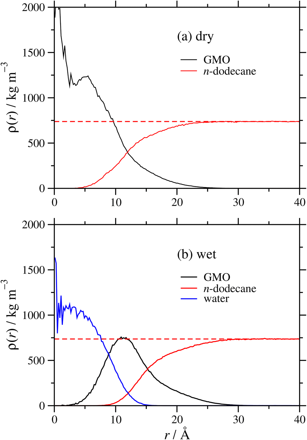 | ||
| Fig. 4 Radial mass-density profiles for GMO (black), dodecane (red), and water (blue) as functions of distance r from the RM centre of mass: (a) the dry system; (b) the wet system with ω = 5. The dashed red lines are fits to the dodecane density for r ≥ 35 Å. | ||
3.3 Self-assembly in solution: MD simulation of many reverse micelles
While a small simulation with a couple of dozen GMO molecules might provide a rough estimate of the size of a self-assembled RM, it would be better to run a simulation with enough GMO molecules to form many micelles. Unfortunately, the number of molecules required to reach a realistic concentration is very large, and at least with atomistic force fields, the atom count would be immense. An MD simulation has been carried out with 1010 GMO molecules, but the concentration is very large, around 83 mM, which is four times higher than in the experiments.A movie of the self-assembly process over a period of 51 ns is provided in the ESI.†Fig. 5 shows the last frame of the large-scale simulation. There are clearly many distinct RMs, with varying apparent sizes due to the instantaneous positions and conformations of molecules, and particularly the tails of the GMO molecules. By eye, a rough estimate of the number of RMs in this snapshot is about 50, corresponding to an aggregation number of 1010/50 ≃ 20.
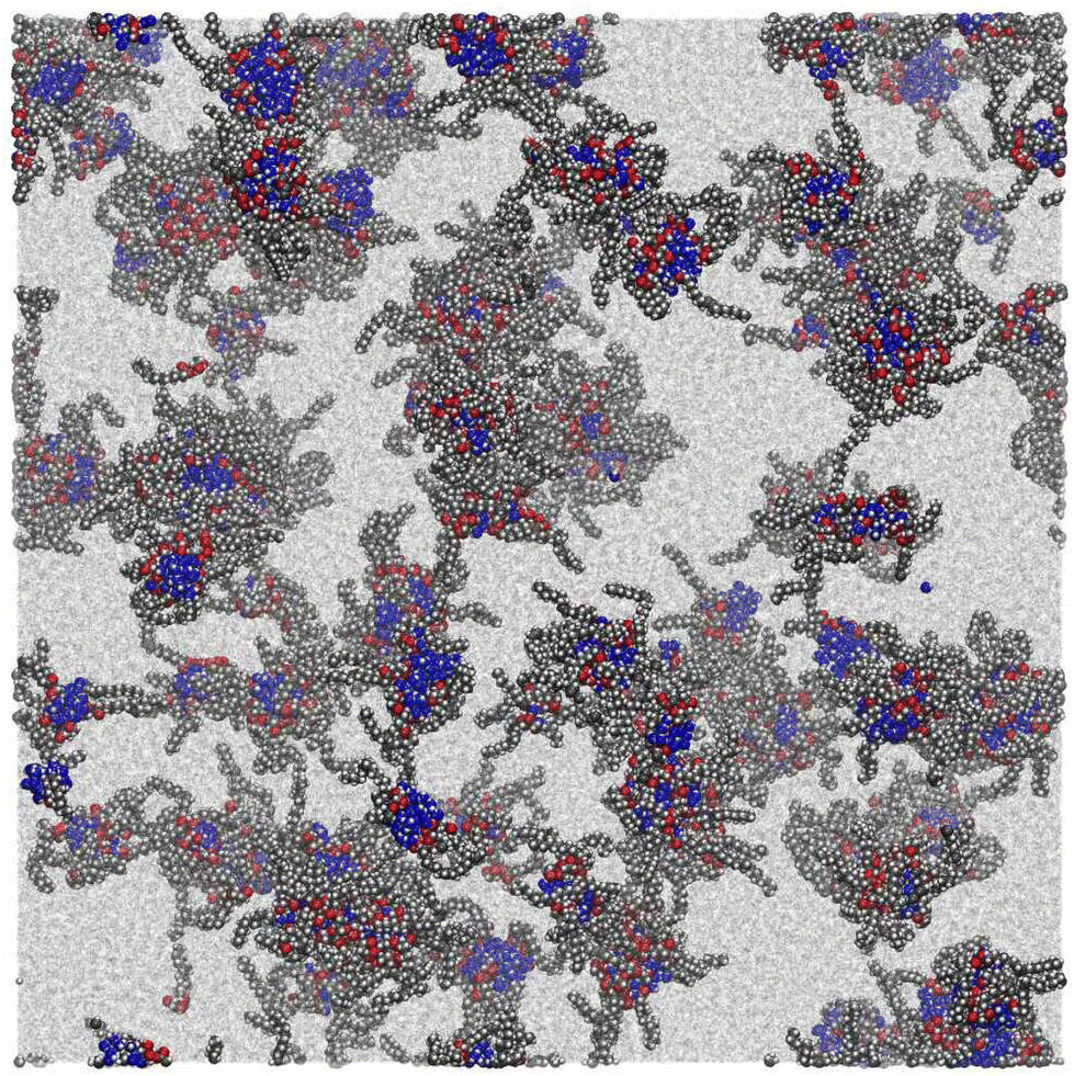 | ||
| Fig. 5 Molecular configuration at the end of a 51 ns run. GMO atoms are shown in space-filling representation, while dodecane is shown in stick representation. GMO carbon atoms are shown in black, GMO oxygens are shown in red, water oxygens are shown in blue, hydrogens are shown in white, and dodecane is shown in grey. | ||
This simulation was run at quite a high GMO concentration, so that the total atom count (including solvent) was kept within reasonable bounds. Early in the self-assembly process, there are many small GMO and water clusters, and individual molecules. (See the movie in the ESI.†) Therefore, to track the kinetics of RM formation, a mixture of cluster and RM criteria would be required to characterise the instantaneous state of aggregation. To circumvent this complication, the kinetics of RM formation were analysed by taking the following ‘experimental’ approach. The 51 ns simulation was split up into 34 1.5 ns chunks, and 16 configurations were saved at intervals of 0.1 ns within each chunk. The level of aggregation was characterised using the atomic structure factor, Satom(Q), computed and averaged for all of the configurations in a chunk.56
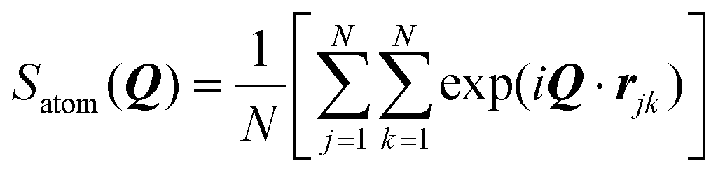 | (9) |
| Satom(Q) = P(Q)S(Q) | (10) |
As already noted, there are several obvious choices for P(Q), as given in eqn (5)–(7); to account for there being discrete atoms in the RMs, and to ensure the limit P(Q → ∞) = 1, the fitting functions were modified to P(Q) = [P(0) − 1]F(Q) + 1, where F(Q) is given by the right-hand sides of those equations. The structure factor needs to reflect that RMs cannot overlap. Adopting a hard-sphere description, and at low RM concentration c, the pair correlation function is simply h(r) = −1 when r ≤ D, and h(r) = 0 otherwise, where D = 2RHS is the hard-sphere diameter.56 This gives the result
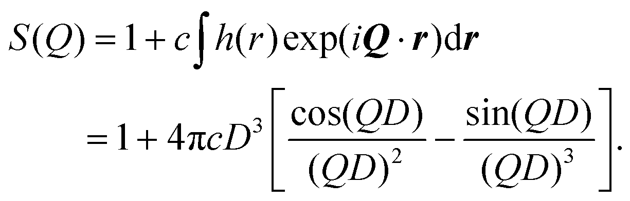 | (11) |
This prescription for S(Q), along with the various options for P(Q), were found to be sufficient for fitting the atomic structure factor Satom(Q). The Percus–Yevick hard-sphere structure factor was also tried,56 but the fitting parameters were hardly affected, which justifies the low-concentration approximation. Each fit yielded values of RHS (and hence Rg) and c.
The effects of the various choices for P(Q) are illustrated in Fig. 6, which shows the fits to the atomic structure factor computed for the final interval between t = 49.5 ns and 51.0 ns. The plot shows three different fits, depending on whether the RM form factor was based on a Gaussian, exponential, or hard-sphere radial atomic density distribution. The exponential distribution gives the best fit, especially so at low-Q and high-Q, and the corresponding value of Rg is within an ångström or so of the direct and fitted values presented in Section 3.2; the factors P(Q) and S(Q) from this fit are also shown in Fig. 6. All of the fitted values of Rg are collected in Table 2. They decrease in the order exponential, Gaussian, and hard sphere, but the fits from the latter two functions are clearly inadequate, especially at high Q, where P(Q) dominates Satom(Q).
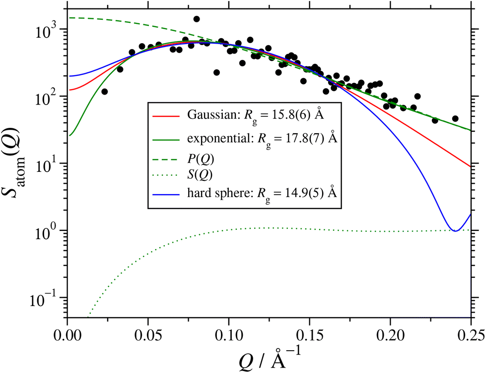 | ||
| Fig. 6 Atomic structure factor Satom(Q) in the interval 49.5 ns ≤ t ≤ 51.0 ns from the large MD simulation. The points are from eqn (9), and lines are fits using eqn (10) with the hard-sphere structure factor (11), and the form factor corresponding to either a Gaussian (5), exponential (6), or hard-sphere (7) radial atomic density distribution; the corresponding values of the radius of gyration Rg are given in the legend. The dashed and dotted lines show, respectively, P(Q) and S(Q) from the exponential fit. | ||
The RM dimensions from the exponential fit are plotted as functions of time in Fig. 7(a) and (b), in terms of both the hard-sphere diameter, and the radius of gyration. The asymptotic values are reached after about 40 ns, and fitting the values for the remaining 11 ns gives hard-sphere and gyration radii of 23 Å and 18 Å, respectively. Fig. 7(c) shows the apparent RM concentration as a function of time, obtained from S(Q) in eqn (11). This decreases with time, as the RMs coalesce and grow. Fitting the exponential function
| c(t) = c(∞) + [c(0) − c(∞)]e−t/τ | (12) |
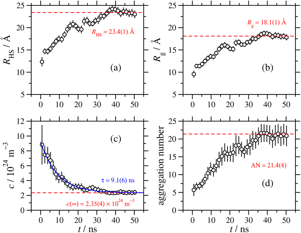 | ||
| Fig. 7 Time-resolved parameters obtained by fitting the atomic structure factor during 1.5 ns intervals of the 51 ns, large MD simulation: (a) the hard-sphere radius of the RM, including a fit from t ≥ 40 ns; (b) the radius of gyration of the RM, including a fit from t ≥ 40 ns; (c) the concentration of RMs, including an exponential fit over the whole time period; (d) the aggregation number, including the asymptotic value obtained from the asymptotic RM concentration shown in (c). | ||
As noted in Section 3.2, a comparison between aggregation numbers from simulation and experiment is unreliable. The sizes of the RMs should be comparable, but the simulated values are lower than the experimental ones by around 7–8 Å. This could be due to the force field, or it could also indicate some longer time scale aggregation processes that are not captured in these simulations. As the MD results show, at the beginning of the aggregation process, there are many small clusters containing a few GMO and water molecules. At longer times, these coalesce into RMs, with well-defined water cores surrounded by GMO molecules. This may not be the thermodynamically stable state, and there could be slower processes akin to Ostwald ripening that lead to the ‘dissolution’ of molecules from small RMs, and subsequent aggregation with larger RMs. These processes are extremely slow (microseconds to seconds), and are beyond the reach of MD simulations.
In future work, it may be possible to parameterise coarse-grained force fields, such as those used in dissipative particle dynamics simulations,57,58 that mimic the specific case of GMO self-assembly. There are some drawbacks of such an approach. Firstly, while generic force fields can reproduce self-assembly as a general phenomenon, the parameters would have to be tuned to reproduce the experimental results, which defeats the object of making predictions. Secondly, water would be substantially coarse-grained in such a force field, and this again militates against chemical fidelity. Finally, such force fields may not be reliable for adsorption, where specific chemical interactions with surfaces are key. This is a significant task that would require dedicated effort, but if successful, it would be possible to extend the simulations to much longer length and time scales.
3.4 Adsorption onto iron oxide surfaces: depletion isotherms
The adsorption of GMO at the iron oxide–dodecane interface at 30, 45, 60, and 70 °C is described by the depletion isotherms shown in Fig. 8. [GMO]eq is the GMO concentration in the supernatant after centrifugation. The data were found to be appropriately modelled by the Langmuir isotherm for monolayer formation | (13) |
lnKads are given in Table 3, and fitting to the equation ΔGads = ΔHads − TΔSads yields an adsorption enthalpy ΔHads = (−3.2 ± 3.0) kJ mol−1 and an adsorption entropy ΔSads = (61.9 ± 9.3) J K−1 mol−1, suggesting that the adsorption of GMO is an entropy-dominated process, possibly connected with the displacement of adsorbed solvent molecules. However, the temperature range is not very large, and so the temperature dependence of Kads and ΔGads may not be very reliable. Nonetheless, the values of ΔGads are comparable to single-molecule adsorption free energies for GMO in similar solvents,59 which range from −25 kJ mol−1 (measured) to −39 kJ mol−1 (simulated). In ref. 59, the experimental values were obtained by fitting an adsorption isotherm to the apparent surface coverages from friction data, and the simulated values were obtained from MD calculations of the potential of mean force (free energy profile) for adsorption.
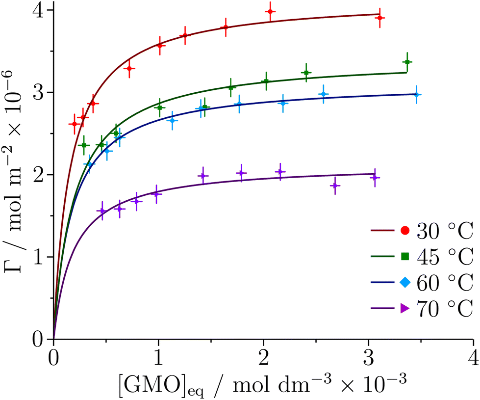 | ||
| Fig. 8 Depletion isotherms for the adsorption of GMO at the iron oxide–dodecane interface at four different temperatures. The solid lines are the best fits of the Langmuir isotherm to the data. | ||
| T/°C | K ads/103 | Γ ∞/Å2 | A mol/10−6 mol m−2 | ΔGads/kJ mol−1 |
|---|---|---|---|---|
| 30 | 6.3 ± 1.0 | 4.2 ± 0.1 | 40 ± 1 | −22.1 ± 0.4 |
| 45 | 5.1 ± 0.9 | 3.4 ± 0.1 | 48 ± 1 | −22.6 ± 0.5 |
| 60 | 5.7 ± 1.1 | 3.1 ± 0.1 | 53 ± 1 | −24.0 ± 0.5 |
| 70 | 5.3 ± 1.5 | 2.1 ± 0.1 | 78 ± 3 | −24.5 ± 0.8 |
The area per molecule was calculated using
 | (14) |
3.5 Adsorption onto iron oxide surfaces: neutron reflectometry of neat dodecane
The small substrate was initially characterised against dodecane-d26 and dodecane-h26 at 25 °C. The reflectivity from each contrast is shown in Fig. 9(a), where the Kiessig fringes mainly arise from both the iron that was deposited on the silicon substrate, and from the native iron oxide which passivates the surface of the iron. A thin layer of amorphous silica is also assumed to have grown on the surface of the silicon substrate prior to coating with iron. The data were co-refined by constraining the substrate parameters to be equal across the contrasts, while the solvent parameters were allowed to vary. Acceptable fits were only achievable with the inclusion of an additional, thin layer at the iron oxide–dodecane interface, referred to as the ‘adventitious layer’. This can be quantified by comparing the natural logarithm of Z for modelling the substrate with (lnZ = 804.8 ± 0.5) and without (lnZ = −177.0 ± 0.5) the adventitious layer, where models with greater Bayesian evidences are preferable. The presence of adventitious material at the iron oxide–dodecane interface has been reported previously,21 and comparable layers have been found at interfaces between materials of high and low surface energy.61–64 The details of this model, including the parameterisation of the adventitious layer and the magnetisation of the iron layer, and the subsequent results, are given in the ESI.†
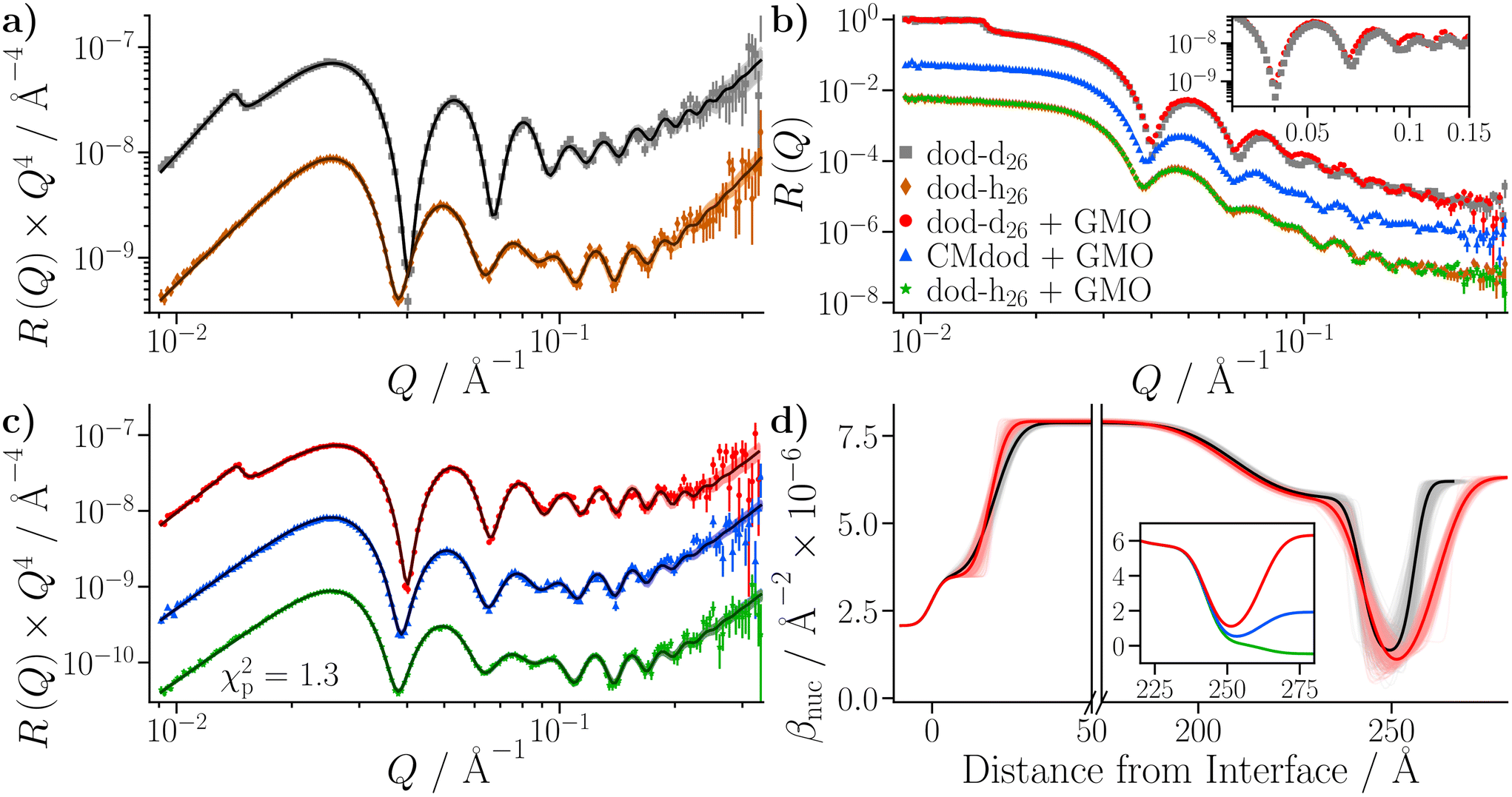 | ||
| Fig. 9 NR data collected with the neat dodecane and GMO–dodecane samples. The legend is located in (b), and the same colours are used throughout. The darker lines represent the profiles using the median values of the parameter distributions, while the shaded bands are comprised of 300 random samples from the posterior distribution. Fits were conducted with Refl1d. (a) NR with the neat dodecane-d26 and dodecane-h26 samples. The reflectivity is multiplied by a factor of Q4 to aid comparison. The contrast collected with dodecane-h26 is scaled by 0.1 in the modified reflectivity axis. (b) Comparison of NR data collected with the GMO–dodecane solutions to the data shown in part (a). The inset compares the modified reflectivity of the two dodecane-d26 contrasts. (c) Fits to the data collected with the 20 mM GMO–dodecane solutions. The contrasts collected with CMdod and dodecane-h26 are scaled by 0.1 and 0.01 in the modified reflectivity axis. (d) The median βnuc profile for the dodecane-d26 contrasts. The inset shows the median βnuc profiles for the three contrasts of the GMO–dodecane system centred on the GMO layer. | ||
3.6 Adsorption onto iron oxide surfaces: neutron reflectometry of GMO in dodecane
Three solutions of GMO in dodecane (20 mM) were prepared with different volumetric ratios of dodecane-d26:dodecane-h26 – 100:0, 65:35, and 0:100. The 65:35 contrast is referred to as silicon contrast-matched dodecane (CMdod). The solution in neat dodecane-d26 was measured first, followed by CMdod and dodecane-h26, exchanged into the same cell. Measurements were taken at 25 °C.
The reflectivities collected with the GMO–dodecane solutions are shown in Fig. 9(b). The dodecane-d26 and dodecane-h26 contrasts are superimposed with the equivalent contrast measured prior to the GMO addition. Three models were proposed to describe the reflectivity, where for each model both the thickness and roughness of the GMO layer were allowed to vary, and either both or one of the nuclear scattering length density, βnuc, and solvation, ϕ, of the GMO layer were also fitted. As in the neat solvent case, the data were co-refined, with the substrate and GMO parameters constrained across the contrasts, while the solvent parameters were allowed to differ. The priors for the GMO layer used in these models, and the estimated Bayesian evidences for each model, are given in Table S9 of the ESI.† The priors for the underlying layers were held constant across these models, and are the same as those given in Table S7 of the ESI.† The model with the greatest evidence had a fixed GMO βnuc, while ϕ was allowed to vary (Model 1 in Table S9†). The fit to the data using this model is shown in Fig. 9(c); the displayed goodness-of-fit statistic is χp2 = χ2/p, where p is the number of data points.
The thickness of the GMO layer was found to be 19.4+1.8−1.6 Å which is less than the extended length of a GMO molecule, estimated to be 23.8 Å, indicating the formation of a film on the monolayer length scale. The thickness of the GMO layer is at least 2 Å greater than that found for the adventitious layer in the neat-solvent contrasts. This difference is evident from the variation in the posterior distributions of the βnuc profiles for the dodecane-d26 contrasts shown in Fig. 9(d). The persistence of adventitious material at the interface is not resolvable when GMO is present as they have similar values of βnuc. The magnetic scattering length density profile is shown in Fig. S3,† and the parameter distributions and correlations are visualised in Fig. S4 of the ESI.†
The molar surface excess of GMO can be calculated by assuming that the layer is comprised solely of GMO and solvent.
 | (15) |
3.7 Adsorption onto iron oxide surfaces: neutron reflectometry of GMO in dodecane with added water
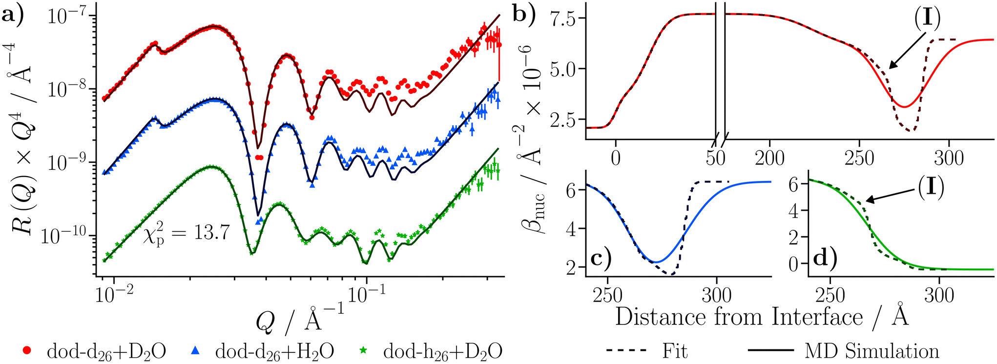
Three water-in-dodecane solutions were prepared with GMO at a concentration of 20 mM, and a hydration ratio ω = 5. Two solutions were prepared with dodecane-d26, which contained either 100% H2O or 100% D2O. The other solution was prepared with dodecane-h26 and 100% D2O. The solutions were passed into a solid–liquid cell containing the larger iron-coated silicon substrate in the order dodecane-d26/H2O, dodecane-d26/D2O, and dodecane-h26/D2O, while the cell was held at 25 °C. The reflectivity from each solvent contrast was measured sequentially, and the resulting profiles are shown in Fig. 10(a). They are compared to the reflectivity from the same substrate held against dodecane-d26 and dodecane-h26. The greatest differences between the reflectivity profiles arise in the dodecane-d26 contrasts. When GMO is present (red and blue) there is a clear difference from the reflectivity measured without GMO (black), which is due to the adsorption of GMO at the interface. There is also a difference between the profiles collected with H2O (blue) and D2O (red), indicating that some water is present at the interface. | ||
| Fig. 10 NR data collected with the dodecane samples stirred with D2O and the GMO–dodecane–water samples. The darker lines represent the profiles using the median values of the parameter distributions, while the shaded bands are comprised of 300 random samples from the posterior distribution. The data shown in parts (a) and (b) are scaled by a factor of Q4 to aid comparison. The legend under part (c) describes the colours used in parts (a)–(c), while the legend under (d) refers to (d) only. (a) Comparison of NR data collected with the GMO–dodecane–water solutions to the data of the dodecane samples that were stirred with D2O. The contrasts collected with dodecane-h26 are scaled by 0.1 in the modified reflectivity axis. (b) The fit of the DL model to the data collected with the GMO–dodecane–water solutions. Fitting was conducted with the PT-MCMC sampler implemented in refnx using 10 temperatures. The dodecane-d26 contrast collected with H2O is scaled by 0.1 and the contrast collected with dodecane-h26 is scaled by 0.01 in the modified reflectivity axis. (c) The βnuc profiles of the dodecane-d26 contrasts. (d) Volume fraction profiles for each component in the DL model. | ||
To infer the structure of the adsorbed material and quantify the surface excesses of GMO and water, the data were modelled. Two models were proposed to describe the reflectivity, referred to as the single layer (SL) model and the double layer (DL) model. Briefly, in the SL model, the interfacial layer is assumed to be a homogeneous mixture of GMO, water, and solvent, while in the DL model, the interfacial region is split into two layers, referred to as the ‘inner’ and ‘outer’ layers. The amounts of GMO, water, and solvent are allowed to differ between these layers, subject to constraints, effectively modelling an inhomogeneous composition of the materials over the surface normal (see the ESI† for further details on the models).
Initial fits to the data, which used Névot–Croce factors to model interfacial roughness, suggested that the iron oxide roughness was larger than the upper bound of the inner layer thickness.66 As such, the typical approach of modelling slab-like layers did not lead to physically-relevant results, and so an approach based on mixing the volume fraction profiles of layers and micro-slicing was used to model the β and reflectivity profiles. Similar approaches have been used to model biological systems.67,68 Further details of the method used here can be found in the ESI.†
Care was taken to ensure that the priors for the underlying substrate structure were consistent between both the SL and DL models; the complete set of priors for both models is given in Table S11 of the ESI.† The Bayesian evidences were found to be lnZ = 479.4 ± 0.6 for the SL model, and lnZ = 593.3 ± 0.6 for the DL model, indicating that the latter model is a better representation of the physical system. The final fit from the DL model is shown in Fig. 10(b), and the resulting βnuc profiles for the water contrasts collected with dodecane-d26 are displayed in Fig. 10(c). The difference between the βnuc profiles mainly arises from the presence of a thin film adsorbed at the iron oxide surface which contains H2O or D2O. A full description of the results is given in the ESI.†
After taking into account the volume occupied by solvent, the volume fractions of GMO within the inner and outer layers were found to be 49.5+6.6−8.4% and 73.0+11.3−4.6%, respectively. Similarly, the water volume fractions in the inner and outer layers were 44.9+6.2−4.7% and 4.3+2.6−2.5%, respectively. The volume fraction profiles, Φi(z), for each component within the model are shown in Fig. 10(d). It is clear that the thin inner layer, which occupies space directly at the interface, is rich in water. Meanwhile the thicker outer layer, that is held at a further distance from the iron oxide surface, mainly consists of GMO. The outer layer contains a small fraction of water, indicating that these water molecules interact with polar GMO head groups found within the outer layer. The volume fraction profiles for GMO and water were calculated following eqn (S17) in the ESI.† The molar surface excesses of GMO and water were calculated separately using an equation of the form
 | (16) |
It was found that the surface excesses were Γ = (4.1 ± 0.1) × 10−6 mol m−2 for GMO, and Γ = (22.8+1.9−1.7) × 10−6 mol m−2 for water. Hence, the areas per molecule were Amol = (41 ± 1) Å2 for GMO, and Amol = (7 ± 1) Å2 for water. In addition, the local hydration ratio within the layer was ω = 5.6+0.6−0.5. Comparing these values to those from the dry GMO–dodecane systems [Γ = (4.7 ± 0.1) × 10−6 mol m−2], it appears that the presence of water suppresses the surface excess of GMO, while slightly swelling the interfacial layer. The molecular-scale mechanism behind this effect is elucidated next.
3.8 Adsorption onto iron oxide surfaces: MD simulations
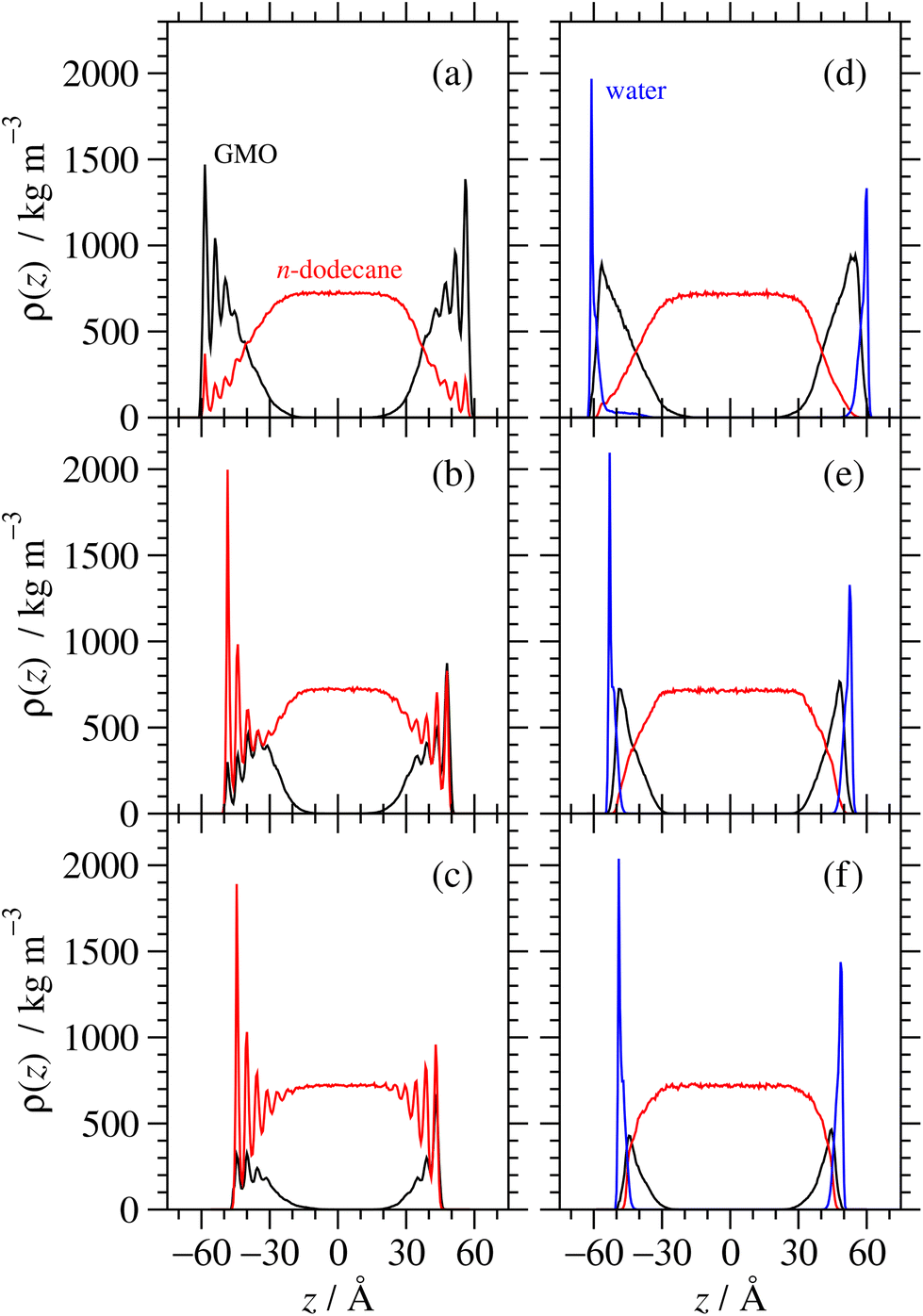
Using the experimentally determined surface excesses from NR, full coverage of both 2775 Å2 iron oxide surfaces required approximately 157 GMO molecules in the dry case, and 137 GMO molecules and 766 water molecules in the wet case. The GMO numbers were rounded off so that they were divisible by 4, in order that ‘full’, ‘half’, and ‘quarter’ coverage simulations could be carried out: these involved 156, 78, and 39 GMO molecules, respectively, in the dry case; and 136, 68, and 34 GMO molecules, respectively, in the wet case. The simulated full coverages were therefore Γ∞ = 4.67 × 10⁻⁶ mol m−2 (dry) and Γ∞ = 4.07 × 10⁻⁶ mol m−2 (wet). 766 water molecules were used in all wet simulations. Final snapshots from each simulation are shown in Fig. 11. In the dry simulations (a)–(c), GMO self-assembly on the surface is signalled by the clusters of oxygen atoms far from the surface, although some head groups are clearly in contact with the surface. In the wet simulations (d)–(f), water forms a strongly adsorbed layer, and there is a GMO-rich layer on top of that. | ||
| Fig. 11 Molecular configurations at the end of 10 ns runs. Parts (a)–(c) show surfaces in dry simulations, and (d)–(f) show surfaces in wet simulations. Parts (a) and (d) represent full GMO coverage, (b) and (e) half coverage, and (c) and (f) quarter coverage. GMO and iron oxide atoms are shown in space-filling representation, while dodecane is shown in stick representation. GMO carbon atoms are shown in black, GMO and surface oxygens are shown in red, water oxygens are shown in blue, hydrogens are shown in white, iron atoms are shown in pink, and dodecane is shown in grey. | ||
Fig. 12 shows mass-density profiles, ρ(z), one for each of GMO, solvent, and water. The dry GMO profiles are oscillatory within 20 Å of the iron oxide surfaces, indicating the atoms in this region have a high degree of order. The extent of ordering decreases at greater distances from the surfaces, so that the profiles decay smoothly beyond the extended length of a GMO molecule (23.8 Å). The presence of GMO atoms beyond this length shows again that some molecules cluster away from the iron oxide surfaces. The extent of layering of the solvent near the surfaces increases with decreasing GMO surface coverage, as the solvent becomes exposed to the surface. The profiles are not perfectly symmetric about z = 0 because the simulations were started from fully disordered configurations, it is not guaranteed that the exact the same number of molecules will adsorb on each surface, and the time scales for desorption and readsorption are so long that increasing the run length will make no difference. For comparison with NR, the profiles for the surfaces were averaged, which cancels out the asymmetry artefact in the profiles.
 | ||
| Fig. 12 Mass density profiles within confined fluid layers. The midplane of each system is defined as z = 0. Parts (a)–(c) are for dry systems, and (d)–(f) are for wet systems. Parts (a) and (d) represent ‘full’ GMO coverage, (b) and (e) ‘half’ coverage, and (c) and (f) ‘quarter’ coverage. | ||
In all cases the systems with water show very different behaviour. Firstly, there is a strongly adsorbed, thin layer of water on each surface. Secondly, the GMO does not exhibit pronounced ordering near the surfaces, showing that it has almost no contact with the solid substrate. Finally, there is practically no layering of the solvent near the surfaces. The system with full surface coverage shows an additional feature, being the presence of water away from the iron oxide surfaces, in what is interpreted as the interiors of surface-adsorbed RMs.
The probability distributions, p(z), for the individual atoms of the hydroxyl groups of GMO on a surface are shown in Fig. 13. There is a slightly higher probability of the H atoms than the O atoms being directly coordinated to the surface, but generally the two profiles are similar. What is more striking is the presence of an extended tail beyond the first thin layer around z = 10 Å, which signals the association of OH groups with each other and/or with water. In the dry systems, there is always such a feature, showing that the GMO molecules self-assemble into RMs. In the wet systems, RMs are formed at full coverage, but on going to half and quarter coverages, the self-assembly disappears, showing that the molecules instead orient with the polar head groups towards the adsorbed water layer.
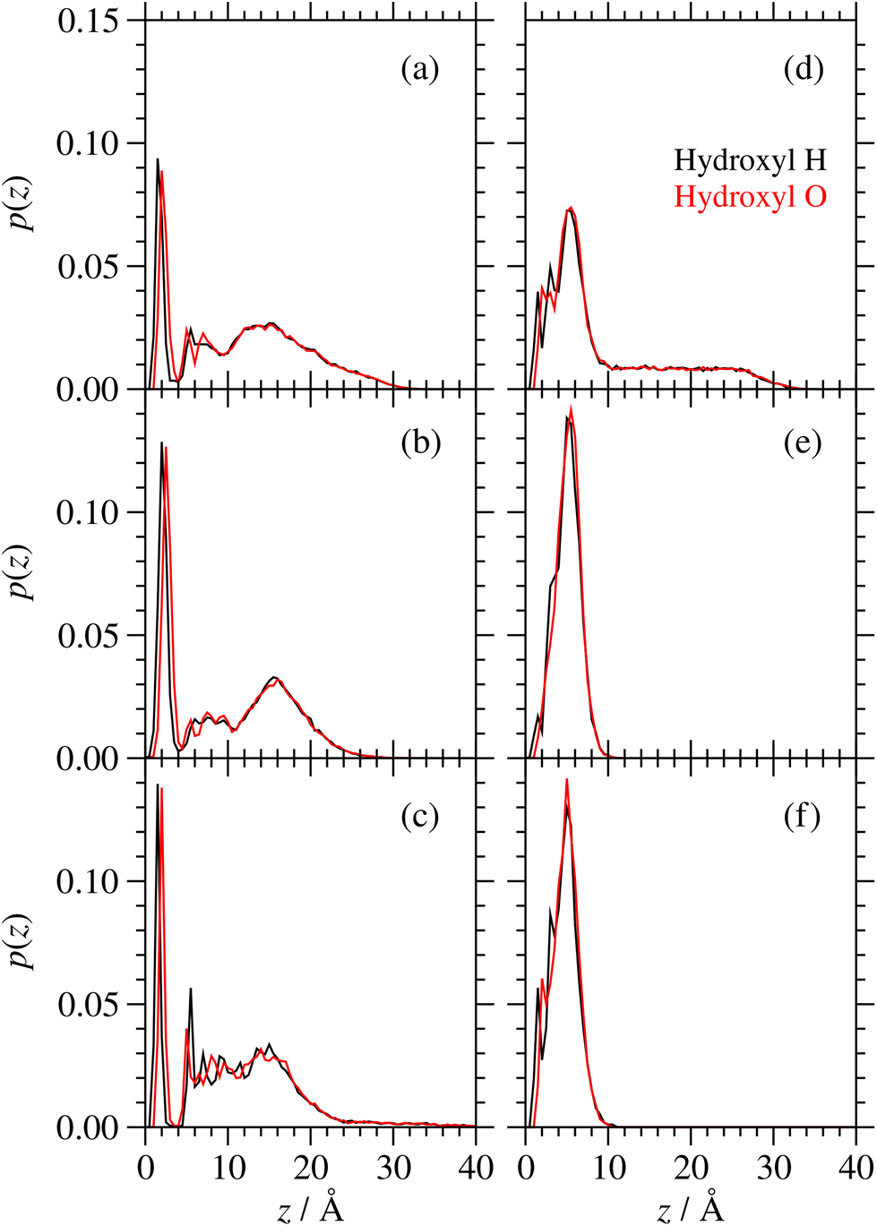 | ||
| Fig. 13 Probability density distribution p(z) of the atoms in the hydroxyl groups of GMO. Parts (a)–(c) are for dry systems, and (d)–(f) are for wet systems. Parts (a) and (d) represent ‘full’ GMO coverage, (b) and (e) ‘half’ coverage, and (c) and (f) ‘quarter’ coverage. | ||
These results show the subtle interplay between self-assembly at the iron oxide–dodecane interface and surface adsorption. In dry systems, most of the molecules are self-assembled into aggregates, but some molecules directly associate with the surface via their polar head groups. In the wet systems, water displaces GMO from the surface. At full surface coverage, GMO can still self-assemble, and even encapsulate some ‘excess’ water, but at lower surface coverages, no self-assembly is evident, and the GMO head groups associate only with the adsorbed water layer. These observations give insights on the change in GMO surface excess on addition of water, as inferred from NR. Next, a direct comparison is made between the measured and computed layer structures.
3.9 Comparison between NR and MD simulations
The general trends inferred from the experimental and MD systems are consistent for both the dry and wet systems. However, to ascertain how the details captured from the MD simulations compare to the experimental system, a direct comparison between the theoretical reflectivity from the MD system and the measured reflectivity is required. To this end, scattering length density profiles β(z) from the MD simulations were calculated by the following routine. First, MD concentration profiles, ni(z), were computed for each atom type i, using the density profile tool from VMD,69 with a bin width of 0.5 Å, and averaged over the last 5 ns of the MD simulation. The profiles for each surface were averaged, and then the scattering length density was computed using | (17) |
Comparison with the NR data requires combination of the measured β(z) profiles of the underlying substrate layers with the computed β(z) profiles from the MD simulation. In the simplest case, the β(z) profiles can be ‘stitched’ together at the interface between the underlying substrate (iron oxide) and the interfacial layers. To do this, the median β(z) profiles from the experimental fit were truncated at the distance at which the median values of βnuc fell below that of the iron oxide layer. The median values of βnuc and the magnetic scattering length density of the iron oxide were then extended to the point at which the iron oxide thickness matched the median thickness from the fits. Beyond this distance, the MD-derived β(z) profiles were stitched onto the iron oxide. For each contrast, the solvent β(z) was scaled so that the mean of β(z) at z ≥ 53.5 Å matched that of the solvent used in the NR experiments. Similar stitching routines have been used previously, and are referred to as ‘splicing’.70,71 The reflectivity from the combined β(z) profiles was then simulated by micro-slicing the profiles into slabs of 0.5 Å.
3.10 Comparison between NR and MD simulations: GMO in dodecane
The simulated reflectivity from the MD simulations is compared to the NR data in Fig. 14(a). The reflectivity was simulated from the spliced β(z) profiles, which are exemplified by the dodecane-d26 contrast shown in Fig. 14(b). The simulated reflectivities of the dodecane-h26 and CMdod contrasts appear to be marginally greater than the measured reflectivity when Q > 0.1 Å−1. This is likely due to the sharp interface between the iron oxide and GMO as modelled in the MD simulations, which appears to be the largest discrepancy between the βnuc profiles shown in parts (c)–(e) of Fig. 14. As described elsewhere,70 any discontinuities within the β profiles lead to significant features in the reflectivity, which would otherwise not be present.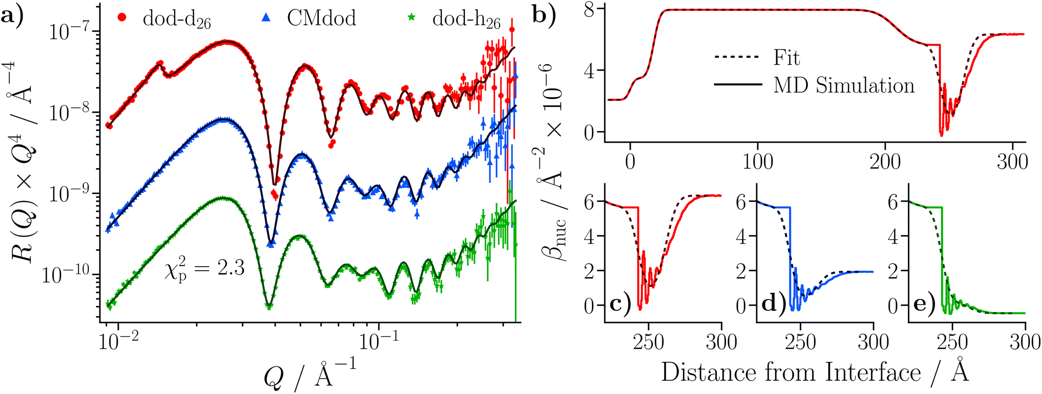 | ||
| Fig. 14 (a) NR data of the GMO–dodecane systems compared to the simulated reflectivity, shown by the solid lines, from the MD simulation. The simulated reflectivity was calculated via the splicing routine. The CMdod and dodecane-h26 contrasts are scaled by 0.1 and 0.01 in the modified reflectivity axis. (b) The βnuc profile of the dodecane-d26 contrast derived from the MD simulation following the splicing routine. This is compared to the median βnuc profile resulting from the original fit shown in Fig. 9(c). Parts (c)–(e) compare the βnuc profiles of all three contrasts over the iron oxide–dodecane interface using the same colour scheme as used in (a). | ||
The effect of the substrate's underlying roughness can be approximated by combining the β(z) profiles from the MD simulations with the inverse of the summed volume fraction profiles of the substrate underlying layers, which represents a cumulative distribution function and is defined as Fsub(z) = 1 − [ΦSi(z) + ΦSiO2 + ΦFe(z) + ΦFeOx(z)]. More specifically, this combination can be calculated as a convolution, which smears the β(z) profiles from the MD simulations due to the underlying substrate roughness.
 | (18) |
 profiles were then added to the β(z) profiles of the underlying substrate calculated from the volume fractions of the underlying substrate. Fig. 15(a) compares the resulting simulated reflectivity to the NR data for all three solvent contrasts, where the largest discrepancy between the data and the simulated reflectivity is in the region Q > 0.1 Å−1 in the dodecane-d26 contrast. This deviation likely arises from a small variation in the structure of GMO and solvent between the simulated and experimental systems. The structural difference can be estimated by comparison of the fitted β(z) profiles and the
  profiles, as shown in Fig. 15(b)–(d) where it appears that the GMO layer as modelled in the fit is denser and less extended than the adsorbed structure found at the end of the MD simulations.
 | ||
| Fig. 15 (a) Simulated reflectivity from the MD simulation after applying convolution compared to the NR data. Part (b) compares the βnuc profile from the fit and from the MD simulations for the dodecane-d26 contrast. Similarly, parts (c) and (d) compare the βnuc profiles of the CMdod and dodecane-h26 contrasts at the iron oxide–dodecane interface. | ||
In this analysis, it is assumed that the roughness of the underlying substrate does not significantly alter the structure of the adsorbed GMO. This assumption is only valid when the horizontal correlation length of the substrate surface is much larger than the horizontal lengths of the cell used in the MD simulation. Therefore, it is possible that some of the discrepancy between the MD-derived reflectivity and the experimental reflectivity arises from the influence of the substrate roughness. In addition, the presence of any impurities, such as trace water, adsorbed at the interface alongside GMO may lead to structural differences between the simulated and measured systems. Furthermore, it is thought that similar structural discrepancies could arise from differences between the iron oxide in the experimental and simulated systems. For example, it is possible that the iron oxide surface is hydroxylated from exposure to the atmosphere.
Convolution has been used previously to smear β profiles of components derived from MD simulations with Gaussian distributions to model their expected out-of-plane fluctuations.70 Although this approach is different to the one taken here, both methods show that convolution is necessary for converting MD-derived structures into appropriate β profiles that can be used for comparison with NR data. Furthermore, the approach used here enables the smearing of volume fractions derived from simulation with non-Gaussian distributions, which can be used to model more complex interfaces between the materials of the underlying substrate.72
3.11 Comparison between NR and MD simulations: GMO in dodecane with added water
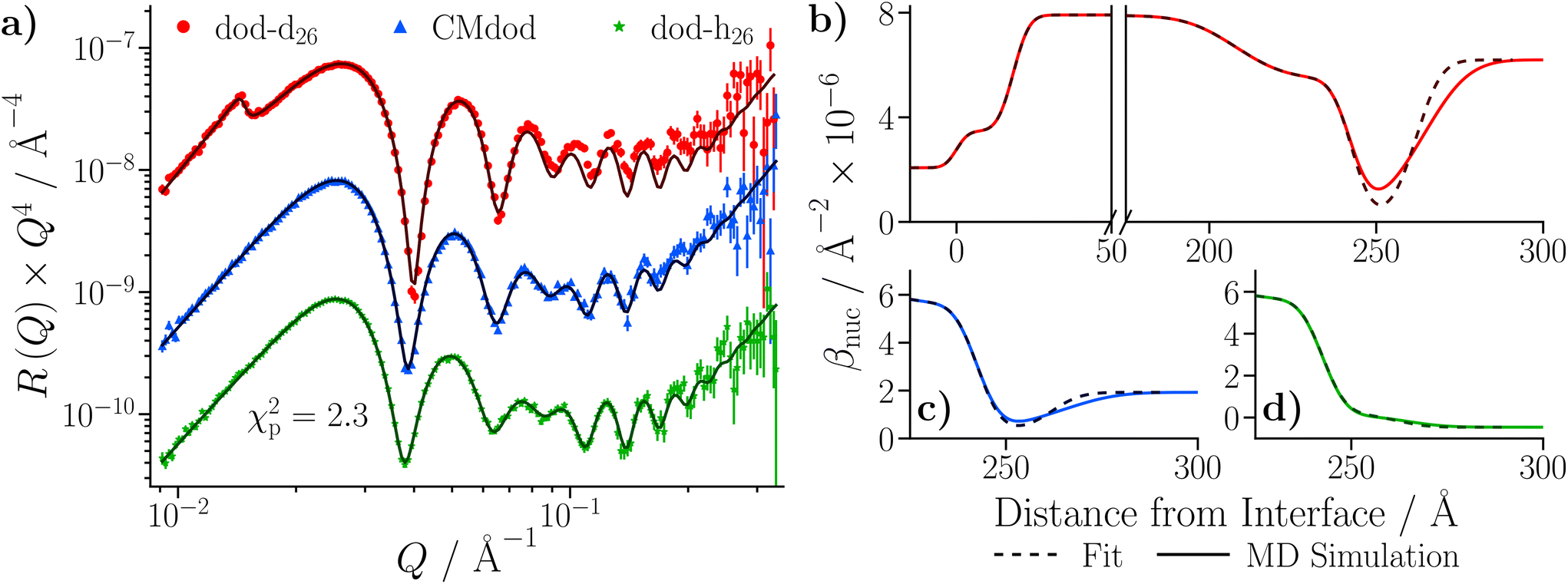
The roughness of the larger substrate was approximately double that of the smaller substrate used in the dry GMO–dodecane systems. Consequently, splicing the MD-derived β profiles onto the median β profiles resulting from the fit would create a much larger discontinuity around the iron oxide–dodecane interface than that shown in Fig. 14(a)–(e). Therefore, only the convolution approach was considered. The β(z) profiles from the MD simulations were convolved with the substrate's underlying roughness following eqn (18). The simulated reflectivity from the profiles was then calculated and is shown in Fig. 16(a). In this case, the largest difference between the measured and simulated reflectivity is the amplitude around Q ∼ 0.1 Å−1 in the dodecane-d26 contrasts; variations in the fringe amplitude can arise from differences in β between the interfacial layers. Fig. 16(b) and (c) show the possible cause of this, where the β of the interfacial layer does not match the β minimum at z ≃ 275 Å from the model fit. Furthermore, it seems the inner layer as modelled in the fit is marginally thicker than the region of high water content found in the MD simulation, evidenced by the slightly higher βnuc around the point marked by (I) in Fig. 16(b) and (d); this is not apparent in part (c) as the βnuc of H2O and GMO are closer in value than when using D2O and GMO. Finally, the fit to the experimental data suggests that the GMO in the outer layer is more dense and less extended than suggested by the MD simulations.
 | ||
| Fig. 16 (a) Comparison of simulated reflectivity from the convolved βnuc profiles, as shown in parts (b)–(d), to the NR data collected with the three dodecane-d26/h26 H2O/D2O contrasts. (b) The βnuc profiles of the dodecane-d26 contrast doped with D2O from the fit and from the convolution approach. Parts (c) and (d) compare the βnuc profiles derived from the fit to those from the convolved MD-derived system for the dodecane-d26 + H2O and dodecane-h26 + D2O contrasts respectively. | ||
4 Conclusions
In this work, a combination of experimental and simulation techniques was used to study the self-assembly and surface adsorption of glycerol monooleate in dodecane, with and without the presence of added water.To study the self-assembly in bulk dodecane, small-angle neutron scattering and molecular dynamics simulations were used to measure the sizes and aggregation numbers of reverse micelles. The effect of added water is to swell the reverse micelles. A large-scale simulation of the self-assembly kinetics, with water, indicated that the rate coefficient for reverse-micelle formation is around 108 s−1. The simulated reverse micelles are smaller than the apparent sizes from small-angle neutron scattering, indicating that there may be slower aggregation processes akin to Ostwald ripening, which are beyond the reach of the simulations.
Depletion isotherms and neutron reflectometry experiments were used to study the amount and structure of glycerol monooleate adsorbed from dry dodecane onto iron-oxide surfaces. The adsorption can be accurately described with a Langmuir isotherm, and the binding free energy is in good agreement with other published values. A sequence of reflectivity experiments was used to explore the adsorbed film structure in both dry and wet systems. Detailed analyses accounting for such factors as impurities, adsorbate molecular orientation, and surface roughness were described. The reflectivity, scattering length density, and volume fraction profiles extracted from the measurements yield the apparent surface excesses, and distributions, of the various adsorbates. Neutron reflectometry data contain information about the laterally-averaged composition of an interface over macroscopic areas (mm2) while the limit of resolution in the normal direction is several ångströms, and so atomistic detail is not obtainable. To this end, simulations with the apparent surface excesses were then carried out, and the structures of the adsorbed films were characterised in detail. Completing the analysis, the simulated structures were converted into scattering length density profiles and simulated reflectivity profiles, which were compared directly with the experimental data. The agreement between experiment and simulation is generally good. Because the simulation results are consistent with the available experimental data, it gives confidence that the atomic-scale modelling provides a reliable picture of the solid–liquid interface. In this case, GMO adsorbs as almost intact reverse micelles, with some molecules coordinating directly to the iron oxide surface through the polar groups. The structure in the wet system appears to be similar with a thin water layer adsorbed at the iron oxide surface. Small amounts of water are also present at further distances from the interface, and interact with the head groups of aggregated GMO molecules. At lower surface coverages, the GMO coordinates directly to the water layer through its polar head groups.
More generally, this exhaustive study shows the power of combining experiments and molecular-simulations in elucidating a rather complex and subtle phenomenon – the interplay between self-assembly and surface adsorption. Firstly, it becomes possible to validate the molecular simulations against experimental measurements; it should be remembered that the adsorbed molecules here are forming layers of only a couple of nanometers thick, and so the comparison is itself quite challenging. Secondly, the resolutions of the experiments and simulations are different, and so they provide complementary information. This combination provides an exquisite level of detail on the solid–liquid interface, and can be used to study a broad range of systems and processes.
This investigation sets the scene for future work on organic friction modifiers, like GMO, under high loads and high shear rates.73 Some interesting behaviour is likely to be revealed under such conditions, which are characteristic of boundary lubrication. As an example, the tribology of adsorbed multilayers of stearic acid is very similar to that of adsorbed monolayers, which suggests that monolayers are responsible for friction modification in both cases, and that additional layers are easily removed under shearing.74,75 In a more complex example, alkyltrimethylammonium chloride surfactants in water form micelles under quiescent conditions, but a transition to a bilayer structure is observed when sheared between mica surfaces.76 In a similar way, adsorbed GMO reverse micelles may disintegrate under high-load, high-shear conditions, and then the friction could be controlled by conventional monolayer adsorption, as in many models of boundary lubrication.77 In any case, the combination of experiments – with the current NR cell operating under shear conditions21 – and molecular simulations will provide valuable insights on such phenomena in situ.
Author contributions
Conceptualization: AJA, RFGA, TMMcC, BNC, PJD, AFR, PJC. Data curation: AJA, RFGA, PJC. Formal analysis: AJA, RFGA, TMMcC, PJC. Funding acquisition: TMMcC, BNC, PJD, AFR, PJC. Investigation: AJA, RFGA, TMMcC, FJA, JD, BNC, PJD, RJLW, AFR, PJC. Methodology: AJA, RFGA, TMMcC, FJA, JD, BNC, PJD, RJLW, AFR, PJC. Project administration: BNC, PJD, AFR, PJC. Resources: BNC, PJD, AFR, PJC. Software: AJA, RFGA, PJC. Supervision: BNC, PJD, AFR, PJC. Validation: AJA, RFGA. Visualization: AJA, RFGA, PJC. Writing – original draft: AJA, RFGA, PJC. Writing – review & editing: AJA, RFGA, TMMcC, FJA, BNC, PJD, RJLW, AFR, PJC.Conflicts of interest
There are no conflicts to declare.Acknowledgements
This work was supported by Infineum UK Ltd through a PhD studentship to AJA, and research fellowships to AJA, RFGA, and TMMcC. TMMcC acknowledges the support of the Ernest Oppenheimer Fund through provision of an Oppenheimer Research Fellowship at the University of Cambridge. The neutron reflectometry data were analysed using the computing resources provided by STFC Scientific Computing Department's SCARF cluster. The authors gratefully acknowledge STFC for the peer-review access to the INTER neutron reflectometer at ISIS (https://doi.org/10.5286/ISIS.E.RB1920367). The authors thank Zlatko Saracevic for conducting the N2 BET sorption analysis. This work used the ARCHER2 UK National Supercomputing Service (https://www.archer2.ac.uk). RFGA and PJC thank Dr Julien Sindt for help with benchmarking, testing, and monitoring the 2-million-atom simulation on ARCHER2, and the Nvidia Corporation for the donation of Titan Xp and Titan V GPUs used in the research. The authors are grateful to the anonymous referees for their constructive comments.Notes and references
- W. Hardy and I. Bircumshaw, Proc. R. Soc. London, Ser. A, 1925, 108, 1–27 CAS.
- F. P. Bowden, J. N. Gregory and D. Tabor, Nature, 1945, 156, 97–101 CrossRef CAS.
- F. P. Bowden and D. Tabor, The Friction and Lubrication of Solids, Oxford University Press, Revised edn, 2001 Search PubMed.
- M. Campana, A. Teichert, S. Clarke, R. Steitz, J. R. P. Webster and A. Zarbakhsh, Langmuir, 2011, 27, 6085–6090 CrossRef CAS PubMed.
- M. H. Wood, R. J. L. Welbourn, T. Charlton, A. Zarbakhsh, M. T. Casford and S. M. Clarke, Langmuir, 2013, 29, 13735–13742 CrossRef CAS PubMed.
- L. R. Griffin, K. L. Browning, C. L. Truscott and S. M. Clarke, J. Phys. Chem. B, 2015, 21, 6457–6461 CrossRef PubMed.
- M. H. Wood, M. T. Casford, R. Steitz, A. Zarbakhsh, R. J. L. Welbourn and S. M. Clarke, Langmuir, 2016, 32, 534–540 CrossRef CAS PubMed.
- M.-P. Pileni, J. Phys. Chem., 1993, 97, 6961–6973 CrossRef CAS.
- M. J. Hollamby, R. Tabor, K. J. Mutch, K. Trickett, J. Eastoe, R. K. Heenan and I. Grillo, Langmuir, 2008, 24, 12235–12240 CrossRef CAS PubMed.
- V. R. Vasquez, B. C. Williams and O. A. Graeve, J. Phys. Chem. B, 2011, 115, 2979–2987 CrossRef CAS PubMed.
- L. K. Shrestha, O. Glatter and K. Aramaki, J. Phys. Chem. B, 2009, 113, 6290–6298 CrossRef CAS PubMed.
- L. K. Shrestha, R. G. Shrestha, M. Abe and K. Ariga, Soft Matter, 2011, 7, 10017–10024 RSC.
- R. G. Shrestha, L. K. Shrestha, K. Ariga and M. Abe, J. Nanosci. Nanotechnol., 2011, 11, 7665–7675 CrossRef CAS PubMed.
- L. K. Shrestha, R. G. Shrestha, K. Aramaki, J. P. Hill and K. Ariga, Colloids Surf., A, 2012, 414, 140–150 CrossRef CAS.
- G. N. Smith, P. Brown, S. E. Rogers and J. Eastoe, Langmuir, 2013, 29, 3252–3258 CrossRef CAS PubMed.
- T. L. Spehr, B. Frick, M. Zamponi and B. Stühn, Soft Matter, 2011, 7, 5745–5755 RSC.
- A. A. Bakulin, D. Cringus, P. A. Pieniazek, J. L. Skinner, T. L. C. Jansen and M. S. Pshenichnikov, J. Phys. Chem. B, 2013, 117, 15545–15558 CrossRef CAS PubMed.
- P. Pitzalis, M. Monduzzi, N. Krog, H. Larsson, H. Ljusberg-Wahren and T. Nylander, Langmuir, 2000, 16, 6358–6365 CrossRef CAS.
- J. L. Bradley-Shaw, P. J. Camp, P. J. Dowding and K. Lewtas, J. Phys. Chem. B, 2015, 119, 4321–4331 CrossRef CAS PubMed.
- J. L. Bradley-Shaw, P. J. Camp, P. J. Dowding and K. Lewtas, Langmuir, 2016, 32, 7707–7718 CrossRef CAS PubMed.
- A. J. Armstrong, T. M. McCoy, R. J. L. Welbourn, R. Barker, J. L. Rawle, B. Cattoz, P. J. Dowding and A. F. Routh, Sci. Rep., 2021, 11, 9713 CrossRef CAS PubMed.
- O. Arnold, J. C. Bilheux, J. M. Borreguero, A. Buts, S. I. Campbell, L. Chapona, M. Doucet, N. Draper, R. Ferraz Leal, M. A. Gigg, V. E. Lynch, A. Markvardsen, D. J. Mikkelson, R. L. Mikkelson, R. Miller, K. Palmen, P. Parker, G. Passos, T. G. Perring, P. F. Peterson, S. Ren, M. A. Reuter, A. T. Savici, J. W. Taylor, R. J. Taylor, R. Tolchenov, W. Zhou and J. Zikovsky, Nucl. Instrum. Methods Phys. Res., Sect. B, 2014, 764, 156–166 CrossRef CAS.
- P. A. Kienzle, J. Krycka, N. Patel and I. Sahin, Bumps (Version 0.9.0), https://bumps.readthedocs.io/en/latest/index.html, 2022 Search PubMed.
- R. B. D'Agostino, Biometrika, 1971, 58, 341–348 CrossRef.
- R. D'Agostino and E. S. Pearson, Biometrika, 1973, 60, 613–622 Search PubMed.
- J. Webster, S. Holt and R. Dalgliesh, Physica B: Condens. Matter, 2006, 385–386, 1164–1166 CrossRef CAS.
- A. R. McCluskey, J. F. K. Cooper, T. Arnold and T. Snow, Mach. Learn.: Sci. Technol., 2020, 1, 035002 Search PubMed.
- I. J. Gresham, T. J. Murdoch, E. C. Johnson, H. Robertson, G. B. Webber, E. J. Wanless, S. W. Prescott and A. R. J. Nelson, J. Appl. Crystallogr., 2021, 54, 739–750 CrossRef CAS.
- J. S. Speagle, Mon. Not. R. Astron. Soc., 2020, 493, 3132–3158 CrossRef.
- A. R. J. Nelson and S. W. Prescott, J. Appl. Crystallogr., 2019, 52, 193–200 CrossRef CAS PubMed.
- P. A. Kienzle, J. Krycka, N. Patel and I. Sahin, Refl1D (Version 0.8.14), https://refl1d.readthedocs.io/en/latest/index.html, 2021 Search PubMed.
- LAMMPS Molecular Dynamics Simulator, https://www.lammps.org, 2023 Search PubMed.
- S. Plimpton, J. Comput. Phys., 1995, 117, 1–19 CrossRef CAS.
- A. P. Thompson, H. M. Aktulga, R. Berger, D. S. Bolintineanu, W. M. Brown, P. S. Crozier, P. J. in't Veld, A. Kohlmeyer, S. G. Moore, T. D. Nguyen, R. Shan, M. J. Stevens, J. Tranchida, C. Trott and S. J. Plimpton, Comput. Phys. Commun., 2022, 271, 108171 CrossRef CAS.
- L. Martínez, R. Andrade, E. G. Birgin and J. M. Martínez, J. Comput. Chem., 2009, 30, 2157–2164 CrossRef PubMed.
- W. Humphrey, A. Dalke and K. Schulten, J. Mol. Graphics, 1996, 14, 33–38 CrossRef CAS PubMed.
- W. L. Jorgensen, J. D. Madura and C. J. Swenson, J. Am. Chem. Soc., 1984, 106, 6638–6646 CrossRef CAS.
- W. L. Jorgensen and J. Tirado-Rives, J. Am. Chem. Soc., 1988, 110, 1657–1666 CrossRef CAS PubMed.
- W. L. Jorgensen, D. S. Maxwell and J. Tirado-Rives, J. Am. Chem. Soc., 1996, 118, 11225–11236 CrossRef CAS.
- W. Damm, A. Frontera, J. Tirado-Rives and W. L. Jorgensen, J. Comput. Chem., 1997, 18, 1955–1970 CrossRef CAS.
- M. L. P. Price, D. Ostrovsky and W. L. Jorgensen, J. Comput. Chem., 2001, 22, 1340–1352 CrossRef CAS.
- S. W. I. Siu, K. Pluhackova and R. A. Böckmann, J. Chem. Theory Comput., 2012, 8, 1459–1470 CrossRef CAS PubMed.
- R. J. Good and C. J. Hope, J. Chem. Phys., 1970, 53, 540–543 CrossRef CAS.
- M. P. Allen and D. J. Tildesley, Computer Simulation of Liquids, Oxford University Press, Oxford, 2nd edn, 2016 Search PubMed.
- S. Nosé, J. Chem. Phys., 1984, 81, 511–519 CrossRef.
- S. Nosé, Mol. Phys., 1984, 52, 255–268 CrossRef.
- W. G. Hoover, Phys. Rev. A, 1985, 31, 1695–1697 CrossRef PubMed.
- W. G. Hoover, Phys. Rev. A, 1985, 34, 2499–2500 CrossRef PubMed.
- R. L. Blake, R. E. Hessevick, T. Zoltai and L. W. Finger, Am. Mineral., 1966, 51, 123–129 CAS.
- H. Berro, N. Fillot and P. Vergne, Tribol. Int., 2010, 43, 1811–1822 CrossRef CAS.
- C. Ayestarán Latorre, J. P. Ewen, C. Gattinoni and D. Dini, J. Phys. Chem. B, 2019, 123, 6870–6881 CrossRef PubMed.
- I.-C. Yeh and M. L. Berkowitz, J. Chem. Phys., 1999, 111, 3155–3162 CrossRef CAS.
- M. Lupkowski and F. van Swol, J. Chem. Phys., 1990, 93, 737–745 CrossRef.
- A. R. McCluskey, J. Chem. Educ., 2023, 100, 4174–4176 CrossRef CAS.
- D. S. Sivia, Elementary Scattering Theory: For X-Ray and Neutron Users, Oxford University Press, 2011 Search PubMed.
- J.-P. Hansen and I. R. McDonald, Theory of Simple Liquids, Academic Press, London, 3rd edn, 2006 Search PubMed.
- A. Vishnyakov, M.-T. Lee and A. V. Neimark, J. Phys. Chem. Lett., 2013, 4, 797–802 CrossRef CAS PubMed.
- M.-T. Lee, A. Vishnyakov and A. V. Neimark, J. Phys. Chem. B, 2013, 117, 10304–10310 CrossRef CAS PubMed.
- P. Navarro Acero, S. Mohr, M. Bernabei, C. Fernández, B. Domínguez and J. P. Ewen, Langmuir, 2021, 37, 14582–14596 CrossRef PubMed.
- S. Brunauer, P. H. Emmett and E. Teller, J. Am. Chem. Soc., 1938, 60, 309–319 CrossRef CAS.
- D. A. Doshi, E. B. Watkins, J. N. Israelachvili and J. Majewski, Proc. Natl. Acad. Sci. U. S. A., 2005, 102, 9458–9462 CrossRef CAS PubMed.
- M. Maccarini, R. Steitz, M. Himmelhaus, J. Fick, S. Tatur, M. Wolff, M. Grunze, J. Janeček and R. R. Netz, Langmuir, 2007, 23, 598–608 CrossRef CAS PubMed.
- P. Gutfreund, M. Wolff, M. Maccarini, S. Gerth, J. F. Ankner, J. Browning, C. E. Halbert, H. Wacklin and H. Zabel, J. Chem. Phys., 2011, 134, 064711 CrossRef PubMed.
- M. Chu, M. Miller and P. Dutta, Langmuir, 2020, 36, 906–910 CrossRef CAS PubMed.
- V. F. Sears, Neutron News, 1992, 3, 29–37 CrossRef.
- L. Névot and P. Croce, Rev. Phys. Appl., 1980, 15, 761–779 CrossRef.
- F. Heinrich and M. Lösche, Biochim. Biophys. Acta, Biomembr., 2014, 1838, 2341–2349 CrossRef CAS PubMed.
- P. Shekhar, H. Nanda, M. Lösche and F. Heinrich, J. Appl. Phys., 2011, 110, 102216 CrossRef PubMed.
- T. Giorgino, Comput. Phys. Commun., 2014, 185, 317–322 CrossRef CAS.
- A. V. Hughes, F. Ciesielski, A. C. Kalli, L. A. Clifton, T. R. Charlton, M. S. P. Sansom and J. R. P. Webster, Acta Crystallogr., Sect. D: Struct. Biol., 2016, 72, 1227–1240 CrossRef CAS PubMed.
- G. Tsagkaropoulou, F. J. Allen, S. M. Clarke and P. J. Camp, Soft Matter, 2019, 15, 8402–8411 RSC.
- M. Svechnikov, D. Pariev, A. Nechay, N. Salashchenko, N. Chkhalo, Y. Vainer and D. Gaman, J. Appl. Crystallogr., 2017, 50, 1428–1440 CrossRef CAS.
- H. Spikes, Tribol. Lett., 2015, 60, 5 CrossRef.
- F. P. Bowden and L. Leben, Philos. Trans. R. Soc., A, 1940, 239, 1–27 CrossRef.
- B. J. Briscoe and D. C. B. Evans, Proc. R. Soc. London, Ser. A, 1982, 380, 389–407 CAS.
- G. Silbert, N. Kampf and J. Klein, Langmuir, 2014, 30, 5097–5104 CrossRef CAS PubMed.
- S. Jahanmir and M. Beltzer, ASLE Trans., 1986, 29, 423–430 CrossRef CAS.
Footnote |
| † Electronic supplementary information (ESI) available: MD force-field parameters; SANS model parameterisation details; SANS fitting results; NR model parameterisation details; NR fitting results; MD simulation movie of GMO self-assembly. See DOI: https://doi.org/10.1039/d3nr05080g |
| This journal is © The Royal Society of Chemistry 2024 |