
 Open Access Article
 This Open Access Article is licensed under a Creative Commons Attribution-Non Commercial 3.0 Unported Licence
Unveiling the crystal and magnetic texture of iron oxide nanoflowers†
Carlos
Moya
 *ab,
Mariona
Escoda-Torroella
ab,
Javier
Rodríguez-Álvarez
ab,
Adriana I.
Figueroa
ab,
Íker
García
a,
Inés Batalla
Ferrer-Vidal
a,
A.
Gallo-Cordova
c,
M.
Puerto Morales
c,
Lucía
Aballe
d,
Arantxa
Fraile Rodríguez
ab,
Amílcar
Labarta
ab and
Xavier
Batlle
*ab
*ab,
Mariona
Escoda-Torroella
ab,
Javier
Rodríguez-Álvarez
ab,
Adriana I.
Figueroa
ab,
Íker
García
a,
Inés Batalla
Ferrer-Vidal
a,
A.
Gallo-Cordova
c,
M.
Puerto Morales
c,
Lucía
Aballe
d,
Arantxa
Fraile Rodríguez
ab,
Amílcar
Labarta
ab and
Xavier
Batlle
*ab
aDepartament de Física de la Matèria Condensada, Universitat de Barcelona, Martí i Franquès 1, 08028 Barcelona, Spain. E-mail: carlosmoyaalvarez@ub.edu; xavierbatlle@ub.edu
bInstitut de Nanociència i Nanotecnologia (IN2UB), Universitat de Barcelona, 08028 Barcelona, Spain
cDepartment of Nanoscience and Nanotechnology, Instituto de Ciencia de Materiales de Madrid (ICMM-CSIC), Sor Juana Inés de la Cruz 3, 28049 Madrid, Spain
dALBA Synchrotron Light Facility, CELLS, 08290 Barcelona, Spain
First published on 3rd January 2024
Abstract
Iron oxide nanoflowers (IONF) are densely packed multi-core aggregates known for their high saturation magnetization and initial susceptibility, as well as low remanence and coercive field. This study reports on how the local magnetic texture originating at the crystalline correlations among the cores determines the special magnetic properties of individual IONF over a wide size range from 40 to 400 nm. Regardless of this significant size variation in the aggregates, all samples exhibit a consistent crystalline correlation that extends well beyond the IONF cores. Furthermore, a nearly zero remnant magnetization, together with the presence of a persistently blocked state, and almost temperature-independent field-cooled magnetization, support the existence of a 3D magnetic texture throughout the IONF. This is confirmed by magnetic transmission X-ray microscopy images of tens of individual IONF, showing, in all cases, a nearly demagnetized state caused by the vorticity of the magnetic texture. Micromagnetic simulations agree well with these experimental findings, showing that the interplay between the inter-core direct exchange coupling and the demagnetizing field is responsible for the highly vortex-like spin configuration that stabilizes at low magnetic fields and appears to have partial topological protection. Overall, this comprehensive study provides valuable insights into the impact of crystalline texture on the magnetic properties of IONF over a wide size range, offering a deeper understanding of their potential applications in fields such as biomedicine and water remediation.
Introduction
Iron oxide nanoparticles (IONP) composed of either magnetite (Fe3O4) or maghemite (γ-Fe2O3) have been the object of many investigations, not only for the understanding of their fundamental properties but also due to their numerous applications.1,2 Their relative ease of production, good magnetic performance, and good biocompatibility have led to their use in a large variety of applications ranging from environmental remediation to biomedical diagnosis and treatment.3–6 Recently, densely packed aggregates of iron-oxide cores arranged as nanoflower-like (IONF) structures have drawn much attention due to the inherent benefit of combining the advantages of nanocrystals and large single-crystals.7,8 The most relevant feature of IONF is that, despite being relatively large and, thus, having a high saturation magnetization, IONF exhibit nearly zero remanence and coercivity, and consequently no aggregation between the aggregates. Therefore, although magnetic hysteresis resembles that of superparamagnetic (SPM) particles, the initial susceptibility is very large, and the aggregates can be fully saturated under a moderate magnetic field. This behaviour may be related to the existence of some exchange coupling between the cores, leading to a superferromagnetic state of the whole superstructure, i.e., magnetic correlation extends beyond the individual nanocrystals.9 The interplay between the demagnetizing field and the magnetic correlation among the cores could lead to high vorticity of the moment arrangement of the nanocrystals to minimize self-magnetic energy and consequently to the nearly zero remnant state. Interestingly, vortex-like states at zero magnetic field were found in nanocrystalline Fe3O4 particles10–13 and other magnetic nanostructures.14The apparent SPM behaviour makes these IONF ideal magnetic platforms for both biomedicine and water remediation purposes since the net magnetization of the IONF can be controlled at will by the application of a weak external magnetic field so that the particle agglomeration is effectively reduced.15–21
Crucial to optimizing IONF designed for the above applications is probing the 3D magnetic texture associated with the actual demagnetized state, an issue that is becoming more cumbersome than expected. The reason is that there are several aspects affecting the demagnetized state of the IONF such as the distribution of sizes and magnetic anisotropy, and the crystallographic texture of the inner cores within the IONF. The interaction between cores can lead to the formation of magnetic superstructures within a single IONF, potentially leading to supramagnetic correlations over several groups of IONF. Hence, a thorough understanding of both the internal crystallographic and magnetic structures of single IONF is essential.
While conventional structural and magnetic measurements are the backbone for a precise understanding of the nanoscopic properties of the IONF, the study of the specific features within the individual IONF is essential to achieve ultimate control over the functionality of the IONF arrangements. This calls for a correlative study combining standard techniques with advanced complementary techniques sensitive to local magnetic texture, such as synchrotron-based Transmission X-Ray Microscopy (TXM) combined with X-ray magnetic circular dichroism (XMCD),22–24 together with numerical calculations that reproduce the experimental results.
This work reports such a study of different-sized IONF synthesized through polyol routes, ranging from 40 to 400 nm. Despite the significant variation in the size of the aggregate, these samples exhibit a consistent crystalline correlation that extends beyond the individual cores yielding high values of both the saturation magnetization and the initial susceptibility, but with almost zero remnant magnetization and coercivity. Magnetic TXM imaging of tens of individual IONF reveals a predominantly demagnetized state, with a seemingly slight correlation between the agglomerate size and the particular magnetic texture. These experimental findings are supported by micromagnetic simulations, where the role of the interplay between the demagnetizing field and the magnetic interactions between neighbouring cores in stabilizing 3D vortex-like spin configurations is unambiguously shown. These results highlight that the manipulation of the crystalline texture of IONF opens new opportunities for designing highly efficient drug delivery carriers with enhanced properties, as well as materials with excellent sorption capacity for environmental remediation.
Results and discussion
Revealing the crystal texture of IONF within a wide range of sizes
As a first step, we determined the crystalline structure of three characteristic samples formed by densely packed multi-core IONF within a wide range of sizes. Samples were prepared by reacting at high temperatures iron chlorides with glycol solvents in presence of organic surfactants following standard methodologies reported elsewhere.2,20,25–27 The IONF size was modified by tuning reaction parameters in the reaction mixture such as temperature, time, and/or reagent concentration (see details in the Methods section). Fig. 1(a–c) displays a gallery of low-magnification Transmission Electron Microscopy (TEM) images of IONF ensembles. These tend to self-assemble onto the C-coated Cu grid avoiding the formation of large aggregates, probably due to the steric forces associated with the surfactants attached to the IONF surface. Fig. 1(d) depicts the size distributions obtained from the TEM images in Fig. 1(a–c): we obtain values of the mean size of 38 ± 10 nm (IONF40), 122 ± 14 nm (IONF100), and 379 ± 135 nm (IONF400) and the relative standard deviation σRSD, within 0.11 and 0.36. Fig. 1(e) shows core size distributions with average sizes around 4–6 nm, regardless of the IONF size.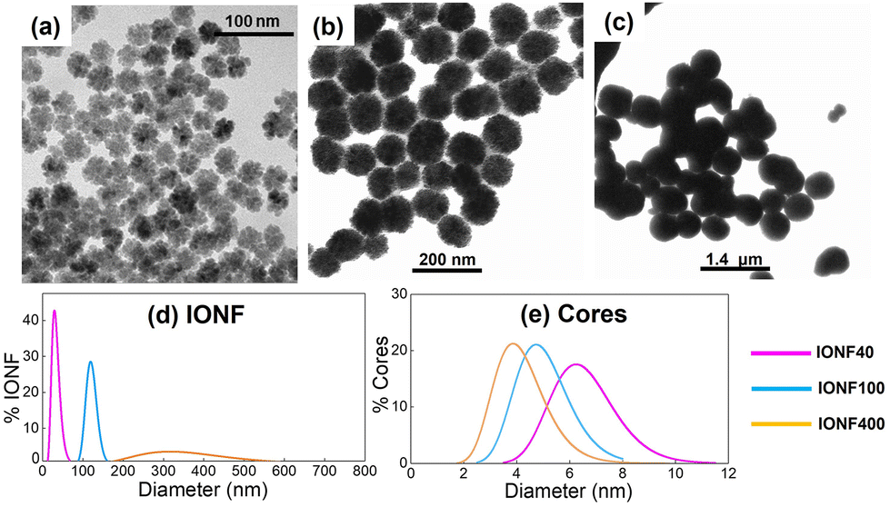 | ||
| Fig. 1 Representative low-magnification TEM images of samples IONF40 (a), IONF100 (b), and IONF400 (c). The size distributions of both IONF aggregates and cores are shown in (d) and (e), respectively. | ||
High-resolution TEM (HRTEM) images depicted in Fig. 2(a), (d) and (g) and in Fig. S1–S3 in the ESI† reveal common trends in the three samples, regardless of IONF size. For example, IONF are composed of multicore aggregates that resemble petal-like nanostructures and interplanar distances consistent with monophasic γ-Fe2O3. Moreover, samples exhibit the same family of planes through large areas of aggregates, which suggests the existence of a crystal correlation between the cores. For example, this is apparent in sample IONF40, where the crystal plane (210) is homogenously distributed over the whole IONF (see Fig. 2(b)). Regarding the crystalline texture of the samples, one would expect Small Angle Electron Diffraction (SAED) patterns for a single IONF to look like those of polycrystalline particles, showing concentric ring-like patterns due to the small size of the cores. However, Fast Fourier transform (FFT) and SAED patterns shown in Fig. 2(c), (f) and (i), corresponding to IONF40, IONF100, and IONF400, respectively, contain a set of relatively ordered spots extending along small arcs of the fully polycrystalline rings. The average angle subtended by the arcs of the spots in the three samples is within 7–14°. This fact indicates that the IONF are neither entirely polycrystalline nor single crystal but show a significant crystalline texture among the cores within each IONF. As expected, the lowest value of the subtended angle is found in sample IONF40, which is made of fewer cores than the other two particle types. Interestingly, although the sample IONF400 contains many more cores than the other two, the average value of the subtended angle is still small, indicating the prevalence of a strong preferential orientation of the cores within the IONF, even in such large core aggregates. This trend can also be visualized by indexing the spots of a SAED pattern of a single IONF400 to the planes oriented in the [111] zone axis of a simulated diffraction pattern of γ-Fe2O3 (see Fig. S4 and Table S1 in the ESI†).
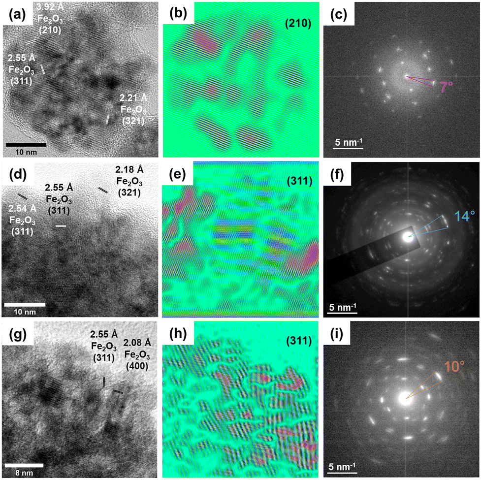 | ||
| Fig. 2 HRTEM characterization of samples IONF40 (a–c), IONF100 (d–f), and IONF400 (g–i). The first column shows HRTEM images indicating the coexistence of several γ-Fe2O3 planes. The second column shows the reconstructed images after performing the inverse FFT of FFT images that were filtered to contain only features associated with plane (210) for sample IONF40, and plane (311) for samples IONF100 and IONF400. The third column shows the calculated FFT pattern (c) obtained from (a) for IONF40, and SAED patterns of single IONF for samples IONF100 (f) and IONF400 (i), respectively. | ||
The crystalline correlation among the cores was further investigated by X-ray diffraction (XRD) (see Fig. 3). At first glance, XRD data show the typical peaks associated with the γ-Fe2O3 phase, ruling out the presence of other parasitic iron oxides phases, such as wüstite (FeO) or hematite (α-Fe2O3).28,29 It is worth mentioning that although these patterns could also be indexed to the Fe3O4 phase, the actual fraction of this phase in the samples, if present, should be very small due to the oxidative acid treatment during the synthesis process (see details in the Methods section). The values of the crystal size determined by the Scherrer method for the three samples are within a small range between 13 and 15 nm.30 Note that these values are more than twice the TEM core sizes, indicating a crystalline order that extends well beyond individual cores. Table 1 summarizes the structural parameters of the three samples obtained from the overall structural characterization techniques.
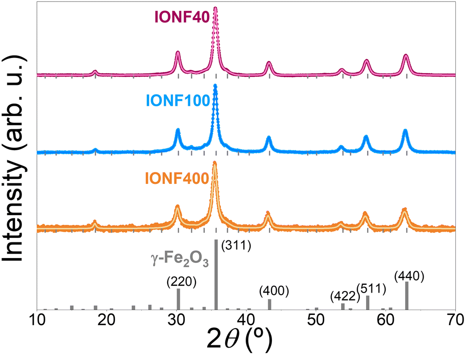 | ||
| Fig. 3 XRD patterns for the series of samples IONF40 (magenta), IONF100 (blue), and IONF400 (orange). For each sample, the dots and solid lines correspond to the experimental data and the fitted curves, respectively. Vertical grey lines at the bottom represent the most intense peaks of the ICSD γ-Fe2O3 pattern: 00-039-1346. | ||
| Sample | D IONF (nm) | σ RSD (%) | D core (nm) | σ RSD (%) | D XRD (nm) |
|---|---|---|---|---|---|
| IONF40 | 38 ± 10 | 26 | 7 ± 1 | 31 | 13 ± 4 |
| IONF100 | 122 ± 14 | 11 | 5 ± 1 | 20 | 15 ± 3 |
| IONF200 | 186 ± 28 | 15 | 20 ± 4 | 20 | 20 ± 3 |
| IONF400 | 379 ± 15 | 36 | 4 ± 1 | 23 | 13 ± 3 |
Correlating the crystal structure with the magnetic properties of the IONF
The crystalline texture of the IONF has a large impact on the magnetic behaviour of the samples. For instance, this is apparent from the hysteresis loops at 298 K (see Fig. 4). Despite the large size of the IONF and their high saturation magnetization MS close to the bulk value (see Table 2), samples show almost zero values of both the remnant magnetization Mr and the coercive field Hc. In addition, the hysteresis loops shown in Fig. 4 for the three samples are quite similar, even though the mean volume of the IONF in samples IONF40 and IONF400 differ by approximately three orders of magnitude. It is worth stressing that, although hysteresis increases as the temperature lowers from room temperature to 5 K, both Mr and Hc remain consistently small (see Fig. S5 in the ESI†). Therefore, the magnetic behaviour of the IONF resembles that of a superparamagnetic NP between room temperature and 5 K, even though IONF are too large to be single domain. So, one could refer to this behaviour as an effective superparamagnetism, since the macroscopic hysteresis loops of our IONF mimic to some extent the salient features of a real superparamagnetic behaviour because of the small values of the remnant magnetization, coercive field, and irreversibility. However, in contrast with actual superparamagnetic behaviour and due to exchange coupling between the cores, IONF may exhibit an ‘effective superferromagnetic state’ with magnetic correlations extending beyond individual nanocrystals that make IONF easily magnetizable under moderate magnetic fields. This exotic phenomenology was further investigated by fitting the magnetization curves at RT to a Langevin function (see Fig. S6 in the ESI†), which is the expected behaviour for a superparamagnetic particle. As shown in Fig. S6,† Langevin functions do not properly follow the abrupt squareness of the curves, and large deviations between the fitting and the experimental data are obtained at the knee of the curves. Note that the magnetization of a superparamagnetic NP typically increases monotonously with the magnetic field, in such a way that saturation cannot be fully reached at any temperature or magnetic field, and the magnetization curves can be scaled onto a single one as a function of the reduced quantity H/T, since they are self-similar.31,32 Therefore, the low values of Mr and Hc in the hysteresis loops of the IONF cannot be attributed to any standard superparamagnetic behaviour. This effective superparamagnetism of the IONF may result from the strong crystalline texture that the cores show in relation to each other, so that magnetic correlations could extend beyond the cores. In fact, previous studies already proposed the existence of some magnetic coupling between the cores, leading to a superferromagnetic state of the whole aggregate, in which magnetic ordering would extend throughout the entire particle.7,8 Magnetic TXM data and micromagnetic simulations discussed below provide a more complete picture of the actual arrangement of the magnetic moments within the individual IONF.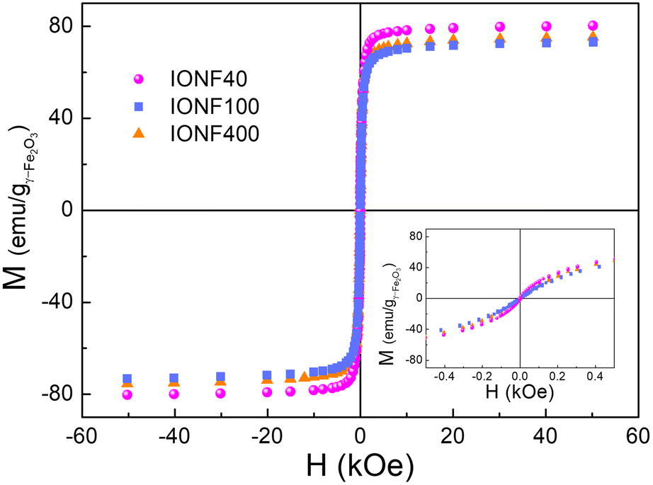 | ||
| Fig. 4 Hysteresis loops at 298 K of samples in powder recorded within H = ±50 kOe. The inset shows the detail corresponding to a small range of the magnetic fields around the origin. Symbols are as follows: IONF40 (magenta solid spheres), IONF100 (blue solid squares), and IONF400 (orange solid triangles). | ||
| Sample | T = 298 K | T = 5 K | ||||
|---|---|---|---|---|---|---|
| M S (emugγ-Fe2O3−1) | M r (emu gγ-Fe2O3−1) | H C (Oe) | M S (emu gγ-Fe2O3−1) | M r (emu gγ-Fe2O3−1) | H C (Oe) | |
| IONF40 | 78 ± 4 | 1.4 ± 0.3 | 4 ± 1 | 87 ± 5 | 14.1 ± 0.5 | 95 ± 3 |
| IONF100 | 70 ± 3 | 0.7 ± 0.2 | 4 ± 1 | 88 ± 4 | 13.4 ± 0.4 | 104 ± 3 |
| IONF200 | 77 ± 5 | 4.6 ± 0.5 | 31 ± 1 | 84 ± 1 | 21.5 ± 1.5 | 227 ± 2 |
| IONF400 | 72 ± 4 | 0.7 ± 0.2 | 2 ± 1 | 88 ± 12 | 10.9 ± 0.5 | 106 ± 3 |
M ZFC/MFC curves as a function of temperature were recorded under H = 50 Oe (see Fig. S7 in the ESI†). They did not show any hint of a blocking temperature, and the onset of irreversibility between the FC and ZFC branches was just at the temperature at which the cooling process started (RT). Additionally, the FC curves exhibited very weak temperature dependence, if any, and no Curie-like increase in magnetization was detected at low temperatures. These results suggest an arrangement of the magnetic moments with significant magnetic correlations throughout the IONF but yielding an almost fully demagnetized state at zero field, similarly to that previously found for nanocrystalline Fe3O4 nanoparticles.33
Imaging of the moment texture in individual IONF
In order to better understand the fully demagnetized state of the IONF shown in Fig. 4, gaining insight into the apparently complex internal magnetic texture of individual NF is required. To this end, a real space characterization of the orientation of the magnetic moments inside the IONF was performed using TXM combined with XMCD as magnetic contrast mechanism17 at the MISTRAL beamline of the ALBA synchrotron.34 All measurements were performed at room temperature in a remnant state following initial out-of-plane magnetic saturation with a magnetic field of 0.3 T applied along the X-ray polarization vector, . Fe L3-edge XMCD images were obtained from the intensity asymmetry ratio of two images recorded with right-(σ+) and left-handed (σ−) circular polarization, (I(σ−) − I(σ+))/(I(σ−) + I(σ+)), at the resonant L3 absorption edge photon energy, which was providing the highest XMCD contrast. Flat field images from blank areas for both polarizations were also recorded and used for normalization. This measurement protocol was repeated for a sequence of XMCD images as a function of the polar angle θ.Fig. 5(a) sketches the geometry used to collect the TXM images. X-ray absorption spectra (XAS) were also obtained in the TXM by collecting successive stacks of images scanning the photon energy. This study was carried out in an intermediate IONF sample, referred to as IONF200, with a DNF of 186 ± 28 nm and a Dcore of 20 ± 4 nm (Fig. S8 in the ESI†). It is worth noting that the distinctive structural features of these agglomerates, characterized by intermediate size and large cores, enable the investigation of the magnetic texture by TXM, with enough spatial resolution within the agglomerate, of 7.7 nm given by the pixel size, while keeping reasonable computing times of the corresponding micromagnetic simulations shown hereafter. The qualitative comparison of the local spectra of individual IONF with those of reference γ-Fe2O3 NP from the literature confirms the maghemite phase across the whole volume of the IONF (Fig. S9 in the ESI†).35 A typical measurement sequence consisted of an average of 60 individual TXM images with an acquisition time of 4 s each. Each image stack obtained from a sequence was then normalized by the flat field image, corrected for sample drifts, and averaged. The results from opposite polarizations were subtracted pixel-by-pixel to yield XMCD contrast images such as the one shown in Fig. 5. Since the dichroic contrast stems only from the magnetization component along the beam propagation direction, a series of XMCD images (Fig. 5(c)) were recorded for selected polar angles, θ = −7.5°, −5°, 0°, 5° and 7.5°. A collection of 53 particles from the selected area shown in Fig. 5(b) and (c) were analyzed. XMCD reflects the projection of the local magnetization
  on the photon propagation vector
  and thus, dissimilar grey levels in Fig. 5(c) correspond to different orientation of the magnetic moments within each individual IONF. The XMCD contrast is proportional to the cosine of the polar angle θ between
  and
and  . Thus, the direction of
  can be extracted from the evaluation of the XMCD intensity in grey scale as a function of θ. Such grey scale was then converted into a scale of moment orientations with respect to the incoming photon beam direction (brightest/darkest contrast corresponding to local magnetic moment parallel/antiparallel to the X-ray beam, 0° and 180°, respectively). The XMCD contrast of single IONF were obtained by extracting the image intensity from square 2 × 2 pixel areas normalized to the corresponding isotropic signal from Fig. 5(b). Following this procedure, we estimated 2D maps of the magnetic moment orientation, each arrow extracted from a 2 × 2 pixel region, that is commensurate with the average core size within the IONF (see Table 1). Note that the XMCD contrast at a fixed θ is insensitive to the change of sign (cos
![[thin space (1/6-em)]](https://www.rsc.org/images/entities/char_2009.gif) θ = cos (−θ)) and, therefore, projections of the local magnetization vector on the upper (0–180°) or lower semicircle (180–360°) appear with the same grey scale in the XMCD images. In our case, 2D magnetization maps were computed by a linear transformation of the image contrast into cosθ considering that all the moments lie in the upper semicircle. This process is repeated for the sequence of XMCD images taken at the other polar angles (θ = −7.5°, −5°, 5° and 7.5°). The XMCD intensity at each pixel displays the expected cosine-like variation with respect to θ (not shown) which serves as consistency check for the obtained local magnetization vectors. Representative 2D maps corresponding to three different single IONF (highlighted with circles in Fig. 5(b) and (c)) are shown in Fig. 6.
θ = cos (−θ)) and, therefore, projections of the local magnetization vector on the upper (0–180°) or lower semicircle (180–360°) appear with the same grey scale in the XMCD images. In our case, 2D magnetization maps were computed by a linear transformation of the image contrast into cosθ considering that all the moments lie in the upper semicircle. This process is repeated for the sequence of XMCD images taken at the other polar angles (θ = −7.5°, −5°, 5° and 7.5°). The XMCD intensity at each pixel displays the expected cosine-like variation with respect to θ (not shown) which serves as consistency check for the obtained local magnetization vectors. Representative 2D maps corresponding to three different single IONF (highlighted with circles in Fig. 5(b) and (c)) are shown in Fig. 6.
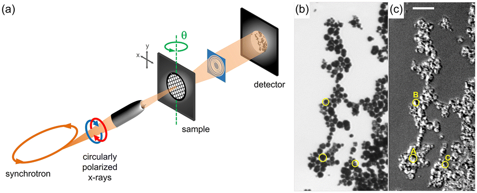 | ||
| Fig. 5 (a) Sketch of the full-field magnetic soft X-ray transmission microscope setup at MISTRAL, depicting the incident X-ray beam/sample geometry with the polar rotation angle θ. (b) Average transmission image recorded for left-circularly polarized X-rays, displaying charge contrast for the particles (dark areas). (c) XMCD image at θ = 0°, where the grey scale level represents the magnetic contrast given by the projection of the magnetic moment along the X-ray beam direction. Bright/dark contrast corresponds to local magnetic moment parallel/antiparallel to the X-ray beam. Yellow circles in (b) and (c) highlight three of the 53 particles analyzed, coined as A, B, and C according to the moment textures found and described in the main text. The scale bar corresponds to 500 nm. | ||
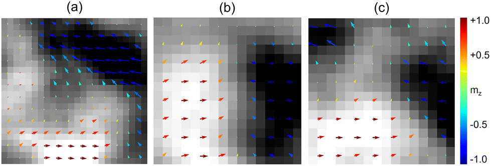 | ||
| Fig. 6 Illustrative examples of magnetic TXM images recorded at polar angle θ = 0° that are representative of the three main categories of moment textures found within the 53 analyzed IONF, labelled as A (a), B (b), and C (c). These particles correspond to those highlighted in Fig. 5(a), and (b). Note that magnetic moments are pointing inwards and outwards the plane for θ angles below and above 90°, respectively, and that the length and direction of the arrow indicate the magnitude and direction of the normalized magnetization vector. | ||
By adding up all the local magnetization vectors within each individual IONF, the net normalized magnetization value, mz, in a scale of −1 to 1 has been obtained. As an example, the IONF in Fig. 6(a) shows a net magnetization of −0.0056, that is, very close to zero corresponding to a demagnetized state. By repeating this process for each of the 53 IONF analyzed, we find that mz as a function of θ for this subset is +0.02 (−7.5°), −0.0057 (0°), +0.034 (5°), and +0.019 (7.5°). Within our statistics, one can conclude that a nearly demagnetized state is thus generally found in IONF, in good agreement with the very low remanence found by macroscopic magnetic characterization of the samples (see Fig. 4, and Fig. S1–S8 in the ESI†), and the micromagnetic simulations that will be shown further below. In addition, as displayed in Fig. S10 in the ESI,† there is no apparent correlation between the IONF size (estimated in pixel units from the TXM images) and mz, which is less than 0.12 in all the cases studied. Note that a precise estimation of the particle size cannot be determined from the TXM images since the spatial resolution is about two orders of magnitude worse than that of the HRTEM images shown in Fig. 2 (0.1 nm spatial resolution from HRTEM vs. 7.7 nm pixel size in TXM).
The analysis performed on the orientation of the local magnetic moments seem to indicate the existence of different types of magnetic textures within individual IONF. Within our subset of 53 particles, three types of spin arrangements within individual IONF have been identified. About 50% of the IONF show a vortex-like configuration with a central tube of magnetization pointing out of the image plane (see Fig. 6(a)), hereafter denoted as type A. About 20% of them, labelled as type B, are compatible with two relatively large black and white regions of somewhat homogeneous magnetization (Fig. 6(b)), resembling magnetic domains. The remaining 30% of IONF fall into an intermediate category, labelled as type C, of black, grey, and white regions of comparable sizes (Fig. 6(c)). Within our error bars, a slight tendency towards more homogeneous textures (such as type B) is observed in IONF with smaller sizes. In contrast, a tendency for more complex twisted moment textures with higher vorticity (such as type A) tends to be found in larger IONF which could be related to increasingly complex correlations between the magnetic moments of the cores associated with their progressively larger number in the aggregate.
OOMMF simulations of a single IONF
To get a deeper understanding into the internal magnetic structure of the IONF yielding the effective superparamagnetism and the magnetic texture found by magnetic TXM experiments, micromagnetic simulations of a model for a single IONF200 were carried out by using OOMMF.36 An approximation to the complex structure of the sample IONF200 was done by building a spheroidal system of 160 nm in diameter made up of nanocubes (NC) of 16 nm in edge length that represent the petals (cores) of the IONF (see Fig. 7). We used a mesh size of 4 nm for the calculations of the unitary moment per cell that allowed to get enough detail in the spatial arrangement inside each core and assign different exchange constants to the cells at the surface of the cores than to those in the interior.
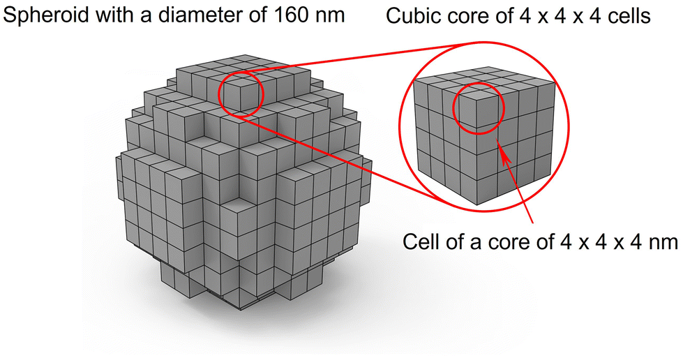 | ||
| Fig. 7 System set up formed building a spheroid of 160 nm in diameter with cubic cores of 16 nm in edge length made up of cells of 4 × 4 × 4 nm. | ||
Both the local arrangement of the moments throughout the IONF and the z-component of the net magnetization of the IONF were studied when a magnetic field was applied along the z-axis following discrete time steps and various convergence criteria to decide when to initiate the next step (see details in the Methods section). In addition, simulations were carried out varying the exchange constant Ai between neighbouring cells in different cores to find out the effect of the inter-core exchange constant on the magnetic configuration of the IONF. As a general trend, the hysteresis loops became more square-like and had higher remnant magnetization and coercivity as Ai increased. Interestingly, the hysteresis loop (see Fig. 8(a)) best resembling that of the real systems was found for Ai = 0.1Aw (Aw being the exchange constant between cells belonging to the same core) thus, this value was selected as a set parameter in the following calculations.
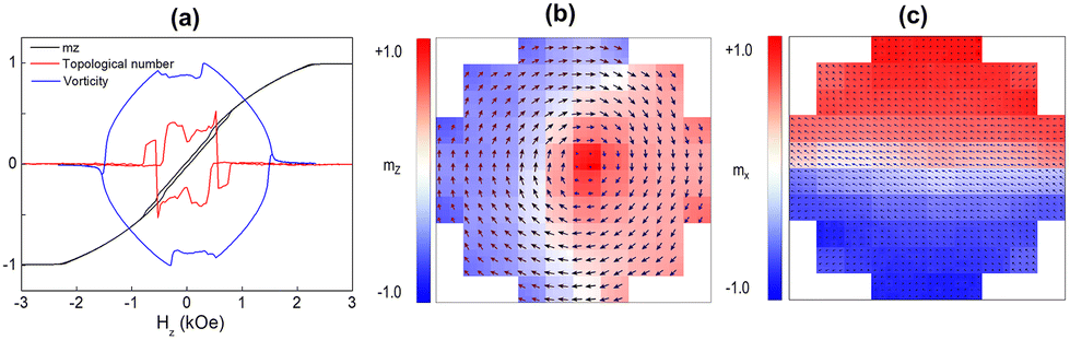 | ||
| Fig. 8 Insights of the OOMF simulations performed for a single IONF. (a) The panel shows normalized magnetization, vorticity, and topological number as a function of the magnetic field for Ai = 0.1Aw. (b) and (c) panels show corresponding snapshots of the moment configuration at remanence for z = 0 and x = 0 planes, respectively. The cell colour represents the sign of the mz/mx component, and the arrow colour stands for the opposite colour map for the sake of an optimum contrast. | ||
One should mention that the same distribution of anisotropies was used in all the simulations shown in this work, and hence, the results were dependent on this realization of the system. Thus, for instance, the detail in the non-reversible part in the hysteresis loop (small jumps and other anomalies) in Fig. 8(a) was related to this configuration of anisotropies. Nevertheless, we checked that other anisotropy distributions gave similar overall behaviour, and only non-significant small differences were found among the results of those simulations. In fact, the system was large enough as to get a kind of self-averaging of the anisotropy disorder.
Regarding the moment arrangements as a function of the applied magnetic field, four stages of the moment configuration following a hysteresis loop are shown in the snapshots in Fig. S11 in the ESI,† corresponding to an equatorial plane perpendicular to the z-axis. At low magnetic field including the remnant states, moment arrangements with high vorticity are found (see Fig. S11(a) and (d) in the ESI† and Fig. 8(b) for remnant states after saturation in opposite directions of the magnetic field). This is because of the combined effects of the demagnetizing field acting in the whole IONF and the weak magnetic interaction between neighbouring cores that causes a certain magnetic correlation among them extending throughout the IONF. This type of complex structure is what gives the system its low remanence and coercivity values, and it vanishes as the system tends to saturation along the field direction. It is also worth stressing that the moments around the central axis of the IONF (along the z-axis) have a significant out-of-plane component (see Fig. 8(c)) of the magnetization, even at remanence. In fact, these central moments form a kind of axial magnetization tube, conferring a certain polarity to the moment vortex that coincides with the direction of the last applied magnetic field (see Fig. 8(c)). In addition, the direction of rotation of the vortex is reversed in the two snapshots at −1.269 kOe in Fig. S11(b) and (c) in the ESI,† since they were simulated while the magnetic field was decreasing and increasing, respectively, before and after saturation along the negative direction of the field axis. It must be pointed out that the moment configurations at remanence (shown in Fig. 8(b) and S8(b) in the ESI†) are in qualitative agreement with the experimental 2D magnetic TXM maps of single IONF labelled as categories A and C (see Fig. 6(a) and (c)). Furthermore, both the vorticity of the moment configuration and the central tube of out-of-plane magnetization are common features found in the OOMMF simulations at remanence and the magnetic TXM data of IONF falling into the categories A and C (Fig. 6(a) and (c)).
Further insight into the vorticity  of the magnetization can be gained by studying
  as a function of the magnetic field. Since
  is a discrete field, a discrete approximation must be taken when calculating the vorticity. Thus, Fig. 8(a) shows the average z-component of the vorticity as the particle follows the hysteresis loop. Notice that abrupt jumps in the magnetization are highly correlated with corresponding changes in the vorticity, as these jumps are the result of reconfigurations of the moment arrangement. In addition, the chirality of the vortex is reversed when the system is saturated and then de-saturated as shown by the snapshots in Fig. S8 in the ESI.† When the applied field is reduced from saturation, the vortex starts to form in the chirality that lowers the energy according to the anisotropy distribution present in the system, which is in opposite directions whether the applied field is increasing or decreasing. At low magnetic fields, vorticity decreases since anisotropies have a more dominant effect in the system, and thus,
  does not align with a perfect vortex.
Topology enables classifying these types of vortex structures. Each  can be viewed as a point on the sphere S2. Therefore, one can map a 2D cross section of the
  configuration to the sphere via the stereographic projection, and classify the mapping from the sphere to the sphere according to how many times it enfolds around itself and computing the topological number W:
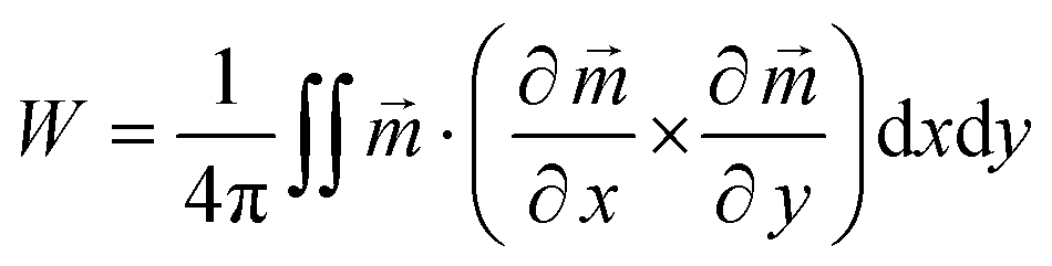 | (1) |
Fig. 8(a) shows W following the hysteresis loop for the equatorial plane shown in Fig. 8(b). Note that there is only non-zero values of W in the non-reversible part of the hysteresis loop. Moreover, W can be viewed as the product of two numbers, which are associated with the net axial polarization of the magnetization and the winding of the moment arrangement. Thus, the abrupt jumps between negative and positive values of W in Fig. 8(a) at Hz = ±0.55 kOe are due to the reversal of the central tube of magnetization along the z-axis, while keeping the direction of the vorticity. Interestingly, a maximum value of W = 0.5 is attained for Ai = 0.1Aw, suggesting that the most stable magnetic structure from the topological point of view takes place for this small value of the inter-core exchange. Thus, although the moment configuration does not attain a complete topologically protected structure at any field, W = 0.5 is remarkably high for a magnetic structure mainly originating from demagnetizing effects and the relatively weak exchange interactions among the cores.
Conclusions
This work shows the effect of the high crystalline texture exhibited by the cores of IONF on the magnetic behaviour of four samples within a wide range of sizes, namely, 40, 100, 200, and 400 nm. Despite the large difference in the IONF sizes, all the samples showed the particularity of having similar crystalline textures among the cores, extending further than twice the core size. This structural correlation was further supported by the relatively small arcs shown by the diffraction patterns of single IONF. As a result of this crystalline texture, there is a certain direct exchange coupling among the moments of neighbouring cores. The combined effect of the magnetic correlation among the cores and the demagnetizing field acting over the whole aggregate causes an effective superparamagnetic behaviour of the IONF. Thus, hysteresis loops showed very small remnant magnetizations and nearly vanishing coercivities while still preserving high values of the saturation magnetization. However, neither the temperature dependence of the magnetization curves followed typical superparamagnetic behaviour nor ZFC magnetization curves showed any hint of a blocking process, suggesting that the system was essentially blocked up to room temperature. Magnetic TXM images of single IONF shed some light on this phenomenology, showing a very small remnant magnetization of the aggregates regardless of their size. In addition, several 3D moment arrangements inside the IONF were observed, ranging from magnetic textures with high vorticity in more than half of the cases to configurations with two seemingly large domains with opposite magnetization. Micromagnetic simulations suggested that there were significant magnetic correlations among the core moments, giving rise to an internal 3D magnetic structure of the IONF with high vorticity that causes an almost fully demagnetized state, in good agreement with the magnetic TXM images. All these results highlight the relevance of IONF as key nanostructured magnetic materials for several biomedical and environmental applications where it is crucial to have magnetic nanocarriers with high values of the magnetization that can be turned on/off by applying/removing an external magnetic field. In particular, the ability to manipulate the crystalline texture of IONF opens new lines for the design of highly efficient drug delivery systems with enhanced properties, such as improved stability, controlled release kinetics, and enhanced targeting capabilities for more effective disease treatment or remote activation of cellular functions. Moreover, precise control over the crystal structure enables the development of IONF-based materials with high sorption capacity, excellent selectivity, and rapid pollutant removal properties, contributing to the purification and remediation of polluted environments.Methods
Synthesis of IONF
IONF samples selected for this work were prepared by the polyol method following wet chemistry routes described by M. P. Morales et.al.2,20,25–27 IONF40 was prepared following the procedure described elsewhere,26 by dissolving 0.3184 g of iron(II) chloride tetrahydrate and 0.8656 g of iron(III) chloride hexahydrate in 64 g of N-methyldiethanolamine and diethylene glycol (50/50 w/w) for 1 h. Afterwards, the pH solution was basified with 0.512 g of sodium hydroxide previously dissolved in 32 g of the solvent mixture. The reaction mixture was left at 190 °C for 8 h in a Teflon lined stainless steel autoclave. The resultant black solution was then washed by magnetic separation several times using an ethyl acetate/ethanol mixture 50/50 v/v, and the precipitate was subjected to an acidic treatment with HNO3 (10%) for 15 min and a thermal treatment with iron(III) nitrate nonahydrate at 80 °C for 45 min to ensure full oxidation of the iron(II) content from Fe3O4 to γ-Fe2O3. Sample IONF100 was prepared by the procedure described in this work.27 For this purpose, 1.3 g of iron(III) chloride hexahydrate, 2.4 g of sodium acetate, and 0.4 g of trisodium citrate were mixed in 40 mL of ethylene glycol under magnetic stirring. Then, the mixture was sealed in a Teflon-lined autoclave and kept at 200 °C for 10 h. After that, the reaction mixture was cooled down to room temperature, washed, and oxidized in a similar manner to sample IONF40. Samples IONF200 and IONF400 were prepared following the procedure described elsewhere with slight modifications.25 Briefly, 0.454 g of iron(III) chloride hexahydrate was dissolved 87 mL in ethylene glycol at 100 °C for 1 h together with 1.38 g of sodium acetate and 6.5 or 3.2 g of PVP20, respectively. The reaction mixture was then transferred to a Teflon-lined autoclave and maintained at 200 °C for 16 h. After cooling down to room temperature, the reaction mixture was washed and oxidized following the above-mentioned conditions.Characterization
TEM samples were prepared by placing a drop of a dilute suspension of IONF in water on a carbon-coated Cu grid and drying for 10 min at 90 °C. TEM measurements were carried out using a JEOL 1010 microscope operating at 100 kV. Histograms of the IONF and the cores were determined by counting at least 300 IONF with ImageJ software and fitted to log–normal distributions following eqn (2).28,37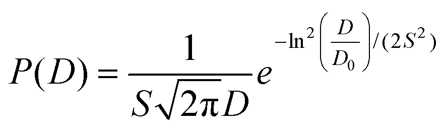 | (2) |
The mean particle size DTEM and the standard deviation σ were computed from eqn (3) and (4), respectively, as follows.
| DTEM = D0eS2/2 | (3) |
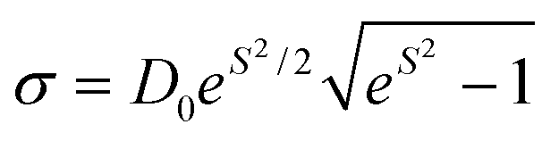 | (4) |
Finally, the diameter dispersion was compared among samples by using the variation coefficient σRSD = σ/DTEM.
The crystal structure of IONF was determined by combining the analysis of HRTEM and SAED patterns obtained with a JEOL 2100 microscope. Interplanar distances (dhkl) were calculated using Gatan Microscopy Suite® software and compared to X'Pert High Score Plus patterns for bulk γ-Fe2O3 (Inorganic Crystal Structure Database, ICSD: 00-039-1346). The interplanar distances of SAED were calculated by measuring the distance between the central spot and the diffraction spots using ImageJ software in at least three different IONF for each sample. The reflections were indexed to the (hkl) planes using the above crystal structure pattern. The representation of the reciprocal lattice at the [111] zone axis was carried out by using CaRIne Crystallography software, version 3.1, and fitting the crystal lattice to the measured SAED area.38
A PANalytical X'Pert PRO MPD diffractometer with Cu Kα radiation (λ = 1.5418 Å) was used to collect XRD spectra within 10° and 70° with a step size of 0.040° of 2θ. The peak positions were compared to a reference spectrum of γ-Fe2O3 (ICSD: 00-039-1346), which was also used to determine the crystal size DXRD by Rietveld analysis of the full spectra using the FullProf Suite software.39
Fe concentration in the colloidal suspensions was determined by Inductively Coupled Plasma Optical Emission Spectroscopy (ICP-OES) with a PerkinElmer OPTIMA 2100 DV by digesting and diluting controlled volumes of samples.
Magnetic features were evaluated in powder samples by measuring hysteresis loops M(H) recorded within ±5T at 5 and 298 K employing a Vibrating Sample Magnetometer (Oxford Instrument Model MLVSM MagLab 9 T). Magnetization values were normalized to the ICP-OES results assuming γ-Fe2O3 phase. Saturation magnetization MS was obtained by extrapolation of the high-field region of M(H) to zero field, assuming the high-field behaviour: M(H) = MS + χpH, where MS and χp correspond to the saturation magnetization and the residual susceptibility due to parasitic paramagnetic species and/or non collinear spin alignments, respectively. Coercive field Hc was computed as Hc = (|Hc+| + |Hc−|)/2, where Hc+ and Hc− were the intercepts of the hysteresis loop branches with the H-axis. Hysteresis loops at 298 K were fitted to a Langevin function (see eqn (5)).40,41
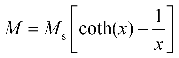 | (5) |
Imaging of the M-TXM in individual IONF was carried out at MISTRAL beamline of the ALBA light source equipped with a full field TXM and a high-precision rotary stage,34 in samples deposited by drop casting onto C-coated marked TEM grids. The two components of the magnetization in the plane perpendicular to the rotation axis were studied in a tomographic series of images using polar angles θ of −7.5°, −5°, 0°, 5°, and 7.5°. To eliminate systematic positioning errors of the goniometer of the microscope, images with both polarizations were acquired sequentially at each angle.
The 2D magnetization maps at given polar angles were studied in 53 IONF using image processing and analysis routines based on ImageJ and homemade python codes.37 All the particles were probed simultaneously, thus, systematic errors arising from either the measurements (e.g., due to an inhomogeneous illumination across the TXM images) or the analysis procedure (mainly caused by image drift correction) were comparable for all the analysed particles. To distinguish the perimeter of each IONF in the XMCD stack, an overlay tool of ImageJ was used as a mask using XAS stacking as reference. Selection of the 53 IONF particles analysed was done after background subtraction of the XMCD image, by cutting each IONF out as a square section with the ImageJ Region of Interest (ROI) tool. The contrast level of each IONF was measured from the mean grey value inside square boxes of 2 × 2 pixels. To visualize the orientation of the magnetic moments inside a selected single IONF in a 2D map of magnetic moments a homemade python program was used to convert the grey scale of the XMCD contrast measurements to a distribution of colour arrows scaling between 0° (red, mz = +1) and 180° (blue, mz = −1).
Numerical calculations (OOMMF code 37) were performed to simulate the internal arrangement of the core moments within a single IONF.36 The real system was approximated by building a 160nm-IONF with small cubes formed by cells of 4 × 4 × 4 nm that mimicked the dimensions of a petal. The exchange constant between cells belonging to the same core was set to Aw = 7 × 10⁻¹² J m−1, which is the value corresponding to bulk maghemite,42 while the exchange constant Ai between neighbouring cells in different cores was set to a percentage of Aw within 5% and 50% in order to account for the inter-core interactions. Therefore, considering that the saturation magnetization for maghemite is Ms = 4.8 × 10⁵ A m−1,42 the chosen cell length of 4 nm is larger or, at most, the same order of magnitude than the magnetostatic correlation length  , supporting the validity of the micromagnetic simulations. There is a significant variability in the shape of the cores in an IONF, so a uniaxial anisotropy axis accounting for the shape and surface anisotropy of each core was chosen randomly, and an average anisotropy constant was set to Ku = −5 × 10³ J m−3, which is a reasonably value for γ-Fe2O3 particles of about tens of nm in size. For the cubic anisotropy, intrinsic to γ-Fe2O3, two unit-vectors were generated for each core, one having a normal distribution around the z-axis with standard deviation of 5°, and the other one perpendicular to it with a uniform distribution of orientations. This was done to account for the important crystalline texture among the cores shown by the IONF. The value of the cubic anisotropy constant was set to Kc = −1.3 × 10⁴ J m−3.42 A white noise that simulated the effect of a temperature of T = 10 K was introduced by a specific routine to reduce the possibility of the system to get stuck in some local minima. When adding a non-zero temperature, criteria based on the convergence of the time derivative of the cell moment were discarded as the fluctuations in the magnetization were greater than any reasonable upper bound. Hence, time criteria were used for the stabilization of the magnetization after any field variation. Given that the path of a hysteresis loop follows metastable states, the results depend on the observation time and the steps taken when varying the applied field. Thus, different stopping times were used for a total number of 320 field steps. The longer the stopping time, the more detail shown in the hysteresis loop, but also the longer total simulation run time. Hence, a stopping time of 5 × 10⁻⁹ s was set as a reasonable compromise between both aspects.
Conflicts of interest
There are no conflicts to declare.Acknowledgements
The financial support from the Spanish MICIIN (grant numbers PGC2018-097789-B-I00, PID2021-127397NB-I00), and PID2020-113480RB-100, Catalan AGAUR (Groups of Excellence 2021SGR00328), and the European Union FEDER funds are greatly recognized. CM acknowledges the funding support from the University of Barcelona and the Spanish Ministry of Universities under the program Maria Zambrano Program founded by the European Union Next Generation-EU/PRTR. Authors are indebted to Luis Fernández-Barquín (U. Cantabria, Spain) for fruitful discussions. Elizabeth M. Jefremovas (U. Cantabria, Spain) is greatly acknowledged for her support during the TXM measurements and Leila Belmonte (UB) for support with development of image analysis routines. The author AIF is a Serra Húnter fellow.References
- X. Batlle, C. Moya, M. Escoda-Torroella, Ò. Iglesias, A. Fraile Rodríguez and A. Labarta, J. Magn. Magn. Mater., 2022, 543, 168594 CrossRef CAS.
- A. G. Roca, L. Gutiérrez, H. Gavilán, M. E. Fortes Brollo, S. Veintemillas-Verdaguer and M. del P. Morales, Adv. Drug Delivery Rev., 2019, 138, 68–104 CrossRef CAS PubMed.
- P. Saharan, G. R. Chaudhary, S. K. Mehta and A. Umar, J. Nanosci. Nanotechnol., 2014, 14, 627–643 CrossRef CAS PubMed.
- N. V. S. Vallabani and S. Singh, 3 Biotech, 2018, 8, 1–23 CrossRef PubMed.
- S. Caspani, R. Magalhães, J. P. Araújo and C. T. Sousa, Materials, 2020, 13, 1–29 CrossRef PubMed.
- Q. A. Pankhurst, J. Connolly, S. K. Jones and J. Dobson, J. Phys. D: Appl. Phys., 2003, 36, R167–R181 CrossRef CAS.
- P. Bender, J. Fock, C. Frandsen, M. F. Hansen, C. Balceris, F. Ludwig, O. Posth, E. Wetterskog, L. K. Bogart, P. Southern, W. Szczerba, L. Zeng, K. Witte, C. Grüttner, F. Westphal, D. Honecker, D. González-Alonso, L. Fernández Barquín and C. Johansson, J. Phys. Chem. C, 2018, 122, 3068–3077 CrossRef CAS.
- P. Bender, D. Honecker and L. Fernández Barquín, Appl. Phys. Lett., 2019, 115, 13 CrossRef.
- Z. W. Tay, S. Savliwala, D. W. Hensley, K. L. B. Fung, C. Colson, B. D. Fellows, X. Zhou, Q. Huynh, Y. Lu, B. Zheng, P. Chandrasekharan, S. M. Rivera-Jimenez, C. M. Rinaldi-Ramos and S. M. Conolly, Small Methods, 2021, 5, 1–10 CrossRef PubMed.
- A. S. Samardak, A. V. Davydenko, A. V. Ognev, Y. S. Jeon, Y. S. Choi and Y. K. Kim, Jpn. J. Appl. Phys., 2016, 55, 100303 CrossRef.
- G. Niraula, D. Toneto, G. F. Goya, G. Zoppellaro, J. A. H. Coaquira, D. Muraca, J. C. Denardin, T. P. Almeida, M. Knobel, A. I. Ayesh and S. K. Sharma, Nanoscale Adv., 2023, 5, 5015–5028 RSC.
- G. R. Lewis, J. C. Loudon, R. Tovey, Y. H. Chen, A. P. Roberts, R. J. Harrison, P. A. Midgley and E. Ringe, Nano Lett., 2020, 20, 7405–7412 CrossRef CAS PubMed.
- H. Gao, T. Zhang, Y. Zhang, Y. Chen, B. Liu, J. Wu, X. Liu, Y. Li, M. Peng, Y. Zhang, G. Xie, F. Zhao and H. M. Fan, J. Mater. Chem. B, 2020, 8, 515–522 RSC.
- P.-C. Elena, M.-V. Samuel, F.-A. Alicia and C. Eugenio, ACS Nano, 2016, 10, 1764–1770 CrossRef PubMed.
- P. Hugounenq, M. Levy, D. Alloyeau, L. Lartigue, E. Dubois, V. Cabuil, C. Ricolleau, S. Roux, C. Wilhelm, F. Gazeau and R. Bazzi, J. Phys. Chem. C, 2012, 116, 15702–15712 CrossRef CAS.
- C. Blanco-Andujar, D. Ortega, P. Southern, Q. A. Pankhurst and N. T. K. Thanh, Nanoscale, 2015, 7, 1768–1775 RSC.
- F. Spizzo, P. Sgarbossa, E. Sieni, A. Semenzato, F. Dughiero, M. Forzan, R. Bertani and L. Del Bianco, Nanomaterials, 2017, 7, 1–15 CrossRef PubMed.
- D. F. Coral, P. A. Soto, V. Blank, A. Veiga, E. Spinelli, S. Gonzalez, G. P. Saracco, M. A. Bab, D. Muraca, P. C. Setton-Avruj, A. Roig, L. Roguin and M. B. Fernández Van Raap, Nanoscale, 2018, 10, 21262–21274 RSC.
- Z. Boekelheide, J. T. Miller, C. Grüttner and C. L. Dennis, J. Appl. Phys., 2019, 126(4), 1–14 CrossRef.
- A. Gallo-Cordova, S. Veintemillas-Verdaguer, P. Tartaj, E. Mazarío, M. D. P. Morales and J. G. Ovejero, Nanomaterials, 2021, 11, 1052–1057 CrossRef CAS PubMed.
- S. Del Sol-Fernández, P. Martínez-Vicente, P. Gomollón-Zueco, C. Castro-Hinojosa, L. Gutiérrez, R. M. Fratila and M. Moros, J. Phys. D: Appl. Phys., 2022, 14, 2091 Search PubMed.
- P. Fischer, T. Eimüller, G. Schütz, P. Guttmann, G. Schmahl, K. Pruegl and G. Bayreuther, J. Phys. D: Appl. Phys., 1998, 31, 649 CrossRef CAS.
- C. Donnelly and V. Scagnoli, J. Phys.: Condens. Matter, 2020, 32, 213001 CrossRef CAS PubMed.
- F. U. H. Wolfgang KuchRudolf, S. P. Fischer and P. Fischer, Magnetic Microscopy of Layered Structures, Springer, Berlin, Heidelberg, 2015 Search PubMed.
- H. Gavilán, E. H. Sánchez, M. E. F. Brollo, L. Asín, K. K. Moerner, C. Frandsen, F. J. Lázaro, C. J. Serna, S. Veintemillas-Verdaguer, M. P. Morales and L. Gutiérrez, ACS Omega, 2017, 2, 7172–7184 CrossRef PubMed.
- A. Gallo-Cordova, J. G. Ovejero, A. M. Pablo-Sainz-Ezquerra, J. Cuya, B. Jeyadevan, S. Veintemillas-Verdaguer, P. Tartaj and M. del P. Morales, J. Colloid Interface Sci., 2022, 608, 1585–1597 CrossRef CAS PubMed.
- H. Gavilán, A. Kowalski, D. Heinke, A. Sugunan, J. Sommertune, M. Varón, L. K. Bogart, O. Posth, L. Zeng, D. González-Alonso, C. Balceris, J. Fock, E. Wetterskog, C. Frandsen, N. Gehrke, C. Grüttner, A. Fornara, F. Ludwig, S. Veintemillas-Verdaguer, C. Johansson and M. P. Morales, Part. Part. Syst. Charact., 2017, 34, 1–12 CrossRef.
- M. Escoda-Torroella, C. Moya, A. F. Rodríguez, X. Batlle and A. Labarta, Langmuir, 2021, 37, 35–45 CrossRef CAS PubMed.
- K. Woo and H. J. Lee, J. Magn. Magn. Mater., 2004, 272–276, 2003–2004 Search PubMed.
- A. L. Patterson, Phys. Rev., 1939, 56, 978–982 CrossRef CAS.
- C. Moya, Ó. Iglesias, X. Batlle and A. Labarta, J. Phys. Chem. C, 2015, 119, 24142–24148 CrossRef CAS.
- N. Pérez, C. Moya, P. Tartaj, A. Labarta and X. Batlle, J. Appl. Phys., 2017, 121, 044304 CrossRef.
- J. S. Lee, J. M. Cha, H. Y. Yoon, J. K. Lee and Y. K. Kim, Sci. Rep., 2015, 5, 1–7 Search PubMed.
- A. Sorrentino, J. Nicolás, R. Valcárcel, F. J. Chichón, M. Rosanes, J. Avila, A. Tkachuk, J. Irwin, S. Ferrer and E. Pereiro, J. Synchrotron Radiat., 2015, 22, 1112–1117 CrossRef CAS PubMed.
- S. Brice-Profeta, M. A. Arrio, E. Tronc, N. Menguy, I. Letard, C. Cartier Dit Moulin, M. Noguès, C. Chanéac, J. P. Jolivet and P. Sainctavit, J. Magn. Magn. Mater., 2005, 288, 354–365 CrossRef CAS.
- M. J. Donahue and D. G. Porter, OOMMF code 37, 1999.
- C. A. Schneider, W. S. Rasband and K. W. Eliceiri, Nat. Methods, 2012, 9, 671–675 CrossRef CAS PubMed.
- Cyrille Boudias & Daniel Monceau, CaRIne Crystallography Software 3.1, 1998 Search PubMed.
- J. Rodriguez-Carvajal and T. Roisnel, Int. Union Crystallogr. Newsletter, 1998, 20, 35–36 Search PubMed.
- C. P. Bean and J. D. Livingston, J. Appl. Phys., 1959, 30, S120 CrossRef.
- W. F. Brown, Phys. Rev., 1963, 130, 1677–1686 CrossRef.
- B. D. Cullity and C. D. Graham, Introduction to Magnetic Materials, 2011 Search PubMed.
Footnote |
| † Electronic supplementary information (ESI) available. See DOI: https://doi.org/10.1039/d3nr04608g |
| This journal is © The Royal Society of Chemistry 2024 |