
 Open Access Article
 This Open Access Article is licensed under a
 Creative Commons Attribution 3.0 Unported Licence
Nonadiabatic molecular dynamics simulations shed light on the timescale of furylfulgide photocyclisation†
Michał Andrzej Kochman ab
ab
aInstitute of Physical Chemistry, Polish Academy of Sciences, Marcina Kasprzaka 44/52, 01-224 Warsaw, Poland. E-mail: mkochman@ichf.edu.pl; Tel: +48 607 989 902
bTheoretical Chemistry, Ruhr University Bochum, Universitätsstraße 150, 44801 Bochum, Germany
First published on 19th July 2024
Abstract
The sequence of events during the photocyclisation of furylfulgides is not fully understood, and there is a significant disparity between ring closing timescales determined with the use of transient absorption spectroscopy [Siewertsen et al., Phys. Chem. Chem. Phys., 2011, 13, 3800] and the timescale estimated on the basis of nonadiabatic molecular dynamics (NAMD) simulations [Kochman et al., Phys. Chem. Chem. Phys., 2022, 24, 18103]. With a view to resolving this issue, in the present study I report NAMD simulations of the photorelaxation process of a model furylfulgide with a bulky alkyl substituent at carbon atom C3. I employed a pattern recognition algorithm in order to automate the analysis of the simulated trajectories. According to the simulation results, the bulky alkyl group causes a substantial increase in the photocyclisation quantum yield, but the timescale of ring closing is only marginally affected. I discuss the implications of these findings in light of the available spectroscopic data.
1 Background
Furylfulgides, also sometimes referred to simply as fulgides, are a class of photochromic compounds with potential applications in several technologies, including rewritable optical memory devices1–7 and photomechanical materials.8,9 The cycle of photoinduced ring-closing and -opening reactions that are responsible for their photochromism is illustrated in Fig. 1 on the following page. Here, 1 represents a series of furylfulgides with different alkyl substituents (R) at carbon atom C3. The open-ring isomers are all colourless, while the closed-ring isomer (C) shows intense red coloration. | ||
| Fig. 1 Molecular structures and photochemistry of furylfulgides in series 1. Atom numbering is shown in blue. R denotes an alkyl substituent at position C3. The box on the bottom right shows the structure of the Eα isomer of furylfulgide 7rF, in which the furyl moiety is tethered to atom C3, preventing rotamerisation into the Eβ isomer. | ||
The first half of the photochromic cycle begins with the Eα isomer. Under irradiation in the ultraviolet (UV) range, this isomer undergoes two parallel photochemical reactions: photocyclisation, which leads to the closed-ring isomer (C), and E → Z photoisomerisation around the C3![[double bond, length as m-dash]](https://www.rsc.org/images/entities/char_e001.gif) C4 bond. The latter process competes with ring closing and, as such, it is an undesired side reaction. Both these reactions are reversible photochemically, but they are thermally irreversible at room temperature.10,11
C4 bond. The latter process competes with ring closing and, as such, it is an undesired side reaction. Both these reactions are reversible photochemically, but they are thermally irreversible at room temperature.10,11
Also involved in the system of reactions that is shown in Fig. 1 is the Eβ isomer, which differs from the Eα isomer in the orientation of the 2,5-dimethyl-3-furyl moiety. In the solution phase, the Eα and Eβ isomers exist in equilibrium with one another.12 Unlike the Eα isomer, the Eβ isomer is incapable of photocyclisation, but it does undergo E → Z photoisomerisation.
The second half of the photochromic cycle is the photoinduced ring-opening reaction (C → Eα), which is triggered by irradiation either in the visible or in the UV range. Normally, light with a wavelength of around 500 nm light is used, which selectively excites the C isomer.13
The mechanisms underlying the photoisomerisation reactions of furylfulgides and related photochromic compounds have been the subject of several spectroscopic13–21 and theoretical20,22–26 studies. Recently, in ref. 25, my co-workers and I investigated the photorelaxation dynamics of the Eα and Eβ isomers of furylfulgide Me-1 (the compound in series 1 with a methyl substituent at position C3) with the use of nonadiabatic molecular dynamics (NAMD) simulations. In that study, it was found that the photoisomerisation reactions of both isomers take place on timescales of hundreds of femtoseconds, and that they do not involve any long-lived reaction intermediates. The accuracy of these simulations was verified through a comparison of the calculated photoisomerisation quantum yields to the experimentally determined photoproduct distribution of furylfulgide Me-127 In this respect, at least, the simulation results obtained in ref. 25 are in agreement with the available experimental data.
However, an unresolved issue is the kinetics of the photocyclisation reaction. In the NAMD simulations carried out in ref. 25, most of the calculated trajectories that underwent ring closing did so at around 200 fs after the initial photoexcitation. This is a somewhat longer timescale than that reported in the transient absorption (TA) spectroscopic study by Siewertsen and co-workers,18 according to whom the ring closing process of furylfulgide Me-1 is characterised by a time constant of roughly 100 fs. In ref. 25, my co-workers and I argued that the time constant of ca. 100 fs is too short to be ascribed to photocyclisation, especially given the fact that this process involves the motion, relative to one another, of two fairly heavy chemical moieties. We hypothesised that this time constant corresponds instead to the initial motion of the nuclear wavepacket away from the Franck–Condon region.25 In any case, even the longer, simulation-based, estimate of the timescale of ring closing places furylfulgide photocyclisation among the fastest known photoisomerisation reactions.28–31
The problem extends to how the timescale of ring closing is affected by the molecular structure. In this regard, it is well documented that the photoproduct distribution (which is a function of the kinetics of the various photorelaxation pathways) is sensitive to the structure of the given furylfulgide.32,33 A series of studies by Yokoyama and co-workers12,27,34 have shown that introducing a bulky alkyl substituent at position C3 has the effect of increasing the quantum yield of the ring-closing reaction, while at the same time decreasing the quantum yield of the undesired E → Z photoisomerisation reaction. A case in point is compound tBu-1 (the compound with a tert-butyl group at position C3), whose photocyclisation quantum yield under irradiation at 366 nm is as high as 0.79.34 Yokoyama and co-workers attributed the decrease in the quantum yield of E → Z photoisomerisation to the fact that full rotation around the C3C4 bond is hindered by steric repulsion between a bulky substituent on atom C3 and the C6Me2 (isopropylidene) moiety.12
Furthermore, Yokoyama et al. hypothesised that an especially bulky substituent at position C3, such as the isopropyl group, causes the molecule to adopt a somewhat different conformation than a smaller substituent, and that this may potentially favour photocyclisation.27 This hypothesis has subsequently found support in the simulation studies by Schönborn and co-workers.23,24
Another spectroscopic study by Siewertsen et al.19 investigated the effect of structural modifications by comparing the excited-state relaxation dynamics of the E isomers of Me-1, iPr-1 (the compound in series 1 with an isopropyl group at position C3), furylfulgide 7rF whose structure is shown in the inset in Fig. 1, and a benzofurylfulgide (a photochromic compound related to furylfulgides in series 1, but with a benzofuryl moiety in place of the furyl moiety). The syntheses and the determination of the photoisomerisation quantum yields of these compounds were described in a separate publication.35 Within the framework of the kinetic model formulated in ref. 19, the time constant for the ring closing process of Me-1 was reported as 110 ± 20 fs. In the case of iPr-1 and 7rF, the time constants for ring closing were reported to be as short as 50 ± 10 fs.19
On the basis of the same argument as was raised previously in ref. 25, the assignment of the extremely short time constants of ca. 50 fs to ring closing seems implausible. This is especially true for compound 7rF, in which the furyl moiety is tethered to atom C3 with an alkyl chain. Obviously, the furyl moiety cannot move independently of the heavy alkyl chain, and this is a factor that is expected to extend the timescale of ring closing. The added mass of the chain may be counteracted to some extent by a pre-orientation effect, which is to say, a ground-state geometry that is favourable to photocyclisation,19,24 but even so, a timescale of ca. 50 fs seems unrealistically short for this compound.
The fact that furylfulgide photocyclisation is one of the fastest known photoisomerisation reactions makes it all the more important to understand its kinetics. In the present study, my aim was to determine the effect of the presence of a bulky substituent on the timescale of ring closing. To this end, I carried out NAMD simulations of the photorelaxation dynamics of tBu-1, a representative furylfulgide with a bulky substituent at position C3. In order to identify the emergent relaxation pathways, I analysed the simulated trajectories with the use of a pattern recognition workflow.
The rest of this paper is organised as follows. In the following section, I outline the computational methodology, with special regard to the pattern recognition analysis. I then discuss the simulation results, beginning with the mechanistic details of the time evolution of the system, and then moving on to a global view of the relaxation process and the main simulation pathways.
2 Computational methods
2.1 Choice of model system
As mentioned in the Background section, the simulations were performed for an isolated molecule of the Eα isomer of furylfulgide tBu-1. This choice of model system was motivated by a number of factors. The first is the high photocyclisation efficiency of tBu-1 – this compound exhibits the highest quantum yield of ring closing from among the five furylfulgides in series 1 for which experimental data are available.32 This suggests that, in tBu-1, the effect of the bulky substituent at position C3 on photoisomerisation kinetics should manifest itself clearly. At the same time, tBu-1 is similar enough in terms of structure to iPr-1, whose relaxation dynamics was studied experimentally by Siewertsen et al.,19 to allow a meaningful comparison of simulation results with spectroscopic data. Also, from the standpoint of simulations, the tert-butyl group is convenient in that it exhibits threefold rotational symmetry, and hence rotations around the C3–tBu bond do not give rise to distinct conformers.As discussed in more detail in Section S1 of the ESI,† the Eα ⇌ Eβ equilibrium of tBu-1 is dominated by the Eα isomer. For this reason, I only performed NAMD simulations for the predominant Eα isomer, and neglected the minority Eβ isomer. The Eβ isomers of furylfulgides are, in any case, incapable of photocyclisation, so modeling the relaxation dynamics of the minority Eβ isomer of tBu-1 is irrelevant to the question of the kinetics of ring closing.
The solvent was not included in the simulations. The neglect of solvent effects is justified by the fact that the spectroscopic measurements reported in ref. 18 and 19 were performed in n-hexane, a non-polar, weakly interacting solvent.
2.2 NAMD simulations
The NAMD simulations modelled the relaxation process of the Eα isomer of tBu-1 following initial photoexcitation into state S1. Their setup mirrored that used previously in ref. 25, in which analogous simulations were performed for the Eα and Eβ isomers of Me-1. Namely, the electronic structure of the molecule was described with the spin–flip variant of time-dependent density functional theory36 (SF-TDDFT), and its dynamics was propagated with the well-known fewest switches surface hopping algorithm.37–39Ntrajs = 50 simulated trajectories were propagated for a period of 500 fs. For ease of reference, a more detailed description of the simulation methodology is provided in the ESI† for this paper. Its accuracy has been thoroughly verified in ref. 25.Owing to the fact that the simulation methodology is exactly the same as in ref. 25, the simulation results can be compared directly to those obtained in the earlier study.
The following parameters were used to describe the relaxation dynamics. The progress of photocyclisation was followed by monitoring the distance between atoms C1 and C6, which is denoted R16. I considered ring closing to have occurred if, at any point during a given simulated trajectory, R16 decreased to less than 1.8 Å.
In different simulated trajectories, ring closing occurs at different time delays after the initial photoexcitation. It is convenient to have a single quantity that serves as a measure of the distribution of ring closing times in the ensemble of trajectories. To this end, I calculated the median of the ring-closing times observed in the simulations.
In some simulated trajectories, the molecule did not undergo photocyclisation, but rather, it followed a reaction path that can be described as unsuccessful E → Z photoisomerisation. Accordingly, I also monitored the torsion angle formed by atoms C2, C3, C4, and C5, which is denoted τ2345. Lastly, I monitored the electronic state of the molecule by following the classical populations of states S0 and S1. As per the usual convention, the classical population (Pj(t)) of the j-th adiabatic state from among those included in NAMD simulations is defined as the fraction of trajectories that is currently evolving in that state:
 | (1) |
2.3 Pattern recognition analysis
NAMD simulations typically produce large amounts of data, which can benefit from analysis with pattern recognition techniques.40–46 In the present case, my goal was to identify the main relaxation pathways that appear in the ensemble of NAMD trajectories. To this end, I designed a pattern recognition workflow in which the set of simulated trajectories was partitioned into clusters of trajectories that are similar to one another, and dissimilar to trajectories in other clusters. I then interpreted each such cluster as a subset of trajectories that follow the same relaxation pathway.For the purposes of the clustering analysis, the state of the molecule along each trajectory was described by a set of three parameters. The first, denoted Q1, was defined as the inverse of the distance between atoms C1 and C6:
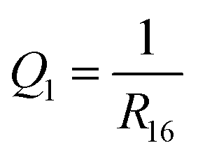 | (2) |
The role of the second parameter, which was denoted Q2, was to monitor rotation around the C3C4 bond. It was defined as the cosine of the torsion angle formed by atoms C2, C3, C4, and C5:
| Q2 = cos(τ2345) | (3) |
Additionally, a third parameter, denoted Q3, was introduced in order to monitor the electronic state of the molecule. If the current state in the given trajectory was state S1, then Q3 was set to the value of the energy gap between states S1 and S0, and if the current state was S0, then Q3 was the negative of the energy gap:
 | (4) |
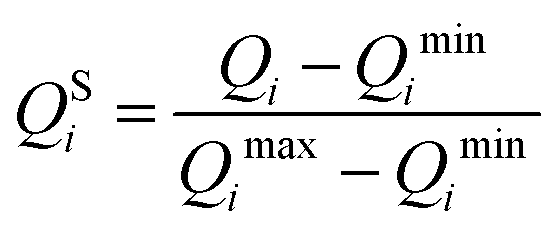
Subsequent analysis required that all three parameters vary on a similar scale and that they are either measured in the same units, or are dimensionless. In order to satisfy both these conditions, prior to further analysis, values of Q1, Q2, and Q3 were each scaled with the standard min–max scaler, which shifts the data in such a way that all features lie in the range [0,1]:
 | (5) |
Each simulated trajectory corresponds to a curve in the three-dimensional Euclidean space spanned by QS1, QS2, and QS3. In what follows, I refer to these three-dimensional curves as the representations of trajectories.
The degree of similarity between pairs of representations of trajectories was quantified with the use of the Fréchet distance47 (FD). The FD is a measure of similarity between curves that takes into account the location and the ordering of points comprising the curves. While the formal definition is mathematically somewhat complex, the FD has a straightforward intuitive definition, which is illustrated in Fig. 2. Imagine a person walking a dog on a leash, such that the person follows a curve I, and the dog follows a curve II. Both curves exist in a metric space, and are finite in length. The dog and its owner can each vary their speed, but they cannot move backwards. Then, the FD between the two curves is the length of the shortest leash that permits the dog and its owner to traverse their respective paths from start to finish. A short FD means that the two curves are similar, and a large FD means they are dissimilar. Note that the value of the FD is symmetric with respect to interchanging the two curves. (The FD is the same regardless of who walks which path.) The FD between any curve and itself is zero.
 | ||
| Fig. 2 Informal definition of the Fréchet distance between paths I and II. See text for details. | ||
Because in the NAMD simulations, the trajectories are discretised at successive time steps, the FD was approximated as the discrete Fréchet distance (DFD).48,49 The calculation of the DFD was performed using the algorithm given by Eiter and Mannila.48
The procedure outlined above yields an Ntrajs × Ntrajs symmetric distance matrix D whose elements Dij are the values of the DFD between pairs of representations of trajectories (i and j). On the basis of the distance matrix, the set of trajectories is partitioned into clusters with the use of the single-linkage clustering algorithm.50 The clustering was performed with the scikit-learn Python library.51
While the choice of parameters Q1 and Q2 is ad hoc in character, the overall procedure is quite general, and can easily be adapted to analyse the results of NAMD simulations for other types of systems.
3 Results and discussion
3.1 Photorelaxation dynamics
For the sake of clarity, the discussion of the simulation results has been split into two subsections. In this subsection, I focus on the mechanistic features of the simulated photorelaxation dynamics of tBu-1. In the following one, I use the pattern recognition analysis to identify the main relaxation pathways that emerge from this data.The time evolution of molecular geometry and the electronic structure is characterised in Fig. 3. In particular, panel (a) shows values of the C1…C6 distance (R16) in the ensemble of simulated trajectories. It can be seen that the simulated dynamics was dominated by ring closing, which took place in 38 of the 50 simulated trajectories. This result is qualitatively in line with the available experimental data, according to which furylfulgide tBu-1 shows a high photocyclisation quantum yield of 0.79 (ref. 34) (this value pertains to tBu-1 in toluene solution, photoexcited at 366 nm).
 | ||
| Fig. 3 Time-evolution of molecular geometry and electronic structure during the relaxation dynamics of the Eα isomer of furylfulgide tBu-1. t = 0 corresponds to the time of the initial photoexcitation. In panel (a), the dashed blue line indicates a C1…C6 distance of 1.8 Å, which I consider as the criterion for ring closing. | ||
The median ring-closing time obtained for furylfulgide tBu-1 is 197 fs. This coincides very closely with the median ring-closing time in the set of simulations reported for Me-1 in ref. 25, which is 201 fs. Thus, it turns out that the presence of a bulky alkyl group at position C3 has only a marginal effect on the timescale of photocyclisation. I will return to this point later on, in Section 3.2.
Fig. 3(b) shows values of the torsion angle formed by atoms C2, C3, C4, and C5 (τ2345) in the ensemble of simulated trajectories. It can be seen that few among the simulated trajectories underwent a substantial rotation around the C3C4 bond. In a single simulated trajectory, τ2345 briefly reached a value of around −90°. In Fig. 3(b), that occurrence is indicated with an arrow. However, the simulation time of 500 fs was too short to determine whether the molecule in that trajectory would go on to undergo a full E → Z photoisomerisation, or whether it would ultimately revert to an E-type geometry. Still, it is evident that the incidence of E → Z photoisomerisation in the simulations must be very low, or zero. This result is in agreement with the experimentally determined photoproduct distribution of furylfulgide tBu-1.34
Panel (c) of Fig. 3 shows the classical populations of states S0 and S1. At the outset of the simulation, the entire ensemble of simulated trajectories was occupying state S1, such that its classical population was equal to unity. The classical population of state S1 remained at a value of 1.0 until around t = 100 fs, at which point it began to decrease rapidly. The sharp drop in the classical population of state S1, and the corresponding rise in the population of state S0, indicates the onset of internal conversion from the former state into the latter. This is due to the photocyclisation reaction: most of the trajectories that underwent ring closing approached the S1/S0 conical intersection seam during a narrow time window between t = 150 fs and t = 300 fs. In doing so, the majority of those trajectories hopped down from state S1 into state S0, and subsequently continued evolving in state S0 for the remaining simulation time of 500 fs.
Complementing this narrative, as part of the ESI† I included animations of ten representative simulated trajectories. Each animation shows the time evolution of molecular geometry, and the energies and populations of states S0 and S1, along the given trajectory. (See Section S2.3 in the ESI† for the definition of the state populations.) The passage of time is indicated with a vertical black line moving along the time axis. The occupied state is marked with a black circle.
3.2 Pattern recognition analysis
I now move on to examine the results of the NAMD simulations through the lens of the pattern recognition algorithm. The structure of the distance matrix D is visualised in Fig. 4. In Fig. 5, the resulting clustering of simulated trajectories is depicted in the form of a dendrogram. | ||
| Fig. 4 Visualisation of distance matrix D whose elements are values of the DFD between representations of simulated trajectories. The value of the DFD is indicated with the use of colour. The trajectories are numbered from 0 to 49. Due to the properties of the DFD, the distance matrix is symmetric, and its diagonal elements are zero. | ||
 | ||
| Fig. 5 Dendrogram representing the single-linkage clustering of simulated trajectories. The trajectories are numbered from 0 to 49. The branches of the tree were assigned colours according to a threshold criterion. All clusters which appear above the threshold are drawn in the same colour (blue). New clusters which appear below the threshold are assigned other colours. The position of the threshold was arbitrarily set to half the maximum DFD between representations of trajectories. | ||
Focusing first on the distance matrix, it can be seen that the values of the DFD show considerable variation: for some pairs of trajectories, the DFD between the representations is near-zero, while for some others, it takes values of up to around 1.1. The large variation in the values of the DFD shows that the trio of parameters Q1, Q2, and Q3 are able to capture the differences between the simulated trajectories. This observation provides a post hoc justification for this choice of parameters. Other than that, it is difficult to analyse the structure of the distance matrix simply by inspection. Hence the need to use a clustering algorithm.
The structure of the dendrogram in Fig. 5 suggests that there are three distinct clusters of trajectories in the ensemble. The largest of the three consists of 26 trajectories out of a total of 50; in Fig. 5, the branch which corresponds to this cluster of trajectories is drawn in red. The inspection of the trajectories allocated to this cluster shows that they all follow the same general sequence of events: the molecule underwent ring closing accompanied by a hop to state S0, and it remained in state S0 for the rest of the simulation. This indicates that the main photorelaxation pathway of tBu-1 is photocyclisation combined with deactivation to the ground electronic state.
One of the smaller clusters of trajectories, which consists of 11 trajectories, and which is drawn in green in Fig. 5, also shows photocyclisation. Here, however, the molecule either did not hop down to state S0, or it spent only a brief time evolving in state S0 before returning again to state S1 through an upward hop. Thus, the simulations predict a second, minor, photorelaxation pathway, one in which photocyclisation takes place without deactivation to the ground electronic state. In this case, the closed-ring isomer is formed in state S1.
The prediction that a substantial fraction of the closed-ring photoproduct is formed in state S1 is not supported by the spectroscopic data reported by Siewertsen and co-workers,18,19 according to which ring closing is accompanied by complete internal conversion to the ground state. For this reason, I do not rule out the possibility that the NAMD simulations have underestimated the incidence of internal conversion to the ground state, and that the formation of some of the closed-ring photoproducts in state S1 is a simulation artifact.
The question presents itself, does this possible simulation artifact affect the calculated timescale of photocyclisation? In order to answer that question, I re-calculated the median ring-closing time, but now taking into account only those trajectories that have been assigned to the main (red) cluster. The median ring-closing time for this subset of simulated trajectories is 204 fs, very close to the value for all trajectories which undergo ring closing. Thus, the possible underestimation of internal conversion to the ground state did not significantly affect the calculated timescale of ring closing. This finding can be explained by noting that the timescale of ring closing is mainly determined by nuclear motions (specifically, the approach of the furyl moiety to atom C6), and not by the electronic dynamics.
The third distinct cluster of simulated trajectories also consists of 11 trajectories; in Fig. 5, it is drawn in orange. The trajectories which comprise this cluster show deactivation to state S0 without photoisomerisation.
It is remarkable that, in compound tBu-1, unproductive deactivation to the ground state is only a minor photorelaxation pathway. Previously, in ref. 25, simulations for compound Me-1 showed that it is actually the predominant outcome, with a quantum yield of 0.64 ± 0.11. Evidently, the replacement of the methyl group at position C3 with the bulkier and more massive tert-butyl group suppresses this relaxation pathway.
The remaining two trajectories which have not been assigned to any of the three main clusters are essentially outliers. In the dendrogram in Fig. 5, these two trajectories appear in blue. One of the two (trajectory no. 7) is a trajectory in which the molecule hopped down into state S0 while undergoing ring closing, evolved in state S0 for around 200 fs, then hopped back into state S1, and remained in that state for the rest of the simulation. Because DFD analysis takes into account the entire history of a given trajectory, this trajectory is identified as an outlier.
The second outlier trajectory (no. 33) is one in which the molecule underwent partial rotation around the C3C4 bond, possibly indicating an instance of E → Z photoisomerisation. However, the simulation time of 500 fs was too short for this process to complete.
Having identified the main photorelaxation pathways, I can estimate the photocyclisation quantum yield of tBu-1. As discussed above, a total of 38 trajectories out of 50 underwent ring closing. Therefore, my simulation-based estimate of the photocyclisation quantum yield is 0.76 ± 0.12. (Here, the confidence interval was estimated with the normal approximation interval52 at the 95% level.)
In ref. 25, the photocyclisation quantum yield of furylfulgide Me-1 was calculated to be 0.27 ± 0.14. (N.B.: this value pertains to isomer Eα alone, that is to say, in the absence of isomer Eβ.) In other words, there is a substantial increase in the quantum of ring closing on going from Me-1 to tBu-1. This increase is not accompanied by a reduction in the timescale of ring closing. Rather, it is achieved by suppressing E → Z photoisomerisation, and nonreactive deactivation to the electronic ground state, which compete with ring closing.
3.3 Implications for kinetics of ring closing
My final order of business will be to tie in the results obtained in the present study and in ref.25 with the available experimental data. As stated in the previous section, the simulations indicate that the photocyclisation quantum yield increases on going from compound Me-1 to tBu-1. This result is consistent with the photocyclisation quantum yields reported by Yokoyama and co-workers.12,27,34On the other hand, the presence of the tert-butyl substituent does not have a significant effect on the timescale of ring closing. Indeed, the median ring-closing time calculated for tBu-1 coincides closely with that predicted for Me-1. In effect, the simulation results indicate that the increase in the photocyclisation quantum yield occurs without a reduction of the timescale of photocyclisation. This finding is compatible with the experimental quantum yields of these compounds. However, it cannot be reconciled with the kinetic model proposed by Siewertsen et al.,13,18 according to which the timescale of ring closing is shorter than in the NAMD simulations, and sensitive to the presence of a bulky substituent at position C3.
In my view, the possibility must be considered that the TA spectroscopic measurements performed by Siewertsen et al.13,18 have not fully resolved the sequence of events during the first few hundred femtoseconds after photoexcitation. That might potentially explain the anomalously short photocyclisation timescales reported for furylfulgides iPr-1 and 7rF. Notwithstanding the above, there seems no reason to doubt the other findings of ref. 13 and 18. The issue appears limited to the earliest events following photoexcitation.
4 Conclusions
In this study, I identified the need for a re-assessment of the spectroscopic data on the kinetics of the photocyclisation reaction of furylfulgides. In order to go some way towards achieving this goal, I undertook to determine whether the timescale of ring closing is affected by the presence of a bulky alkyl substituent at position C3. To that end, I modelled the photorelaxation dynamics of compound tBu-1, and I compared the simulation results to those obtained previously25 for compound Me-1.In the event, it turns out that the timescale of ring closing does not change to a significant extent on going from Me-1 to tBu-1. The apparent lack of sensitivity to the presence of a bulky substituent at position C3 stands in contrast to the findings of the studies by Siewertsen and co-workers,18,19 who reported that a bulky substituent reduces the timescale of ring closing. I interpret this discrepancy as supporting my contention that these studies have not fully resolved the very earliest events during the photorelaxation dynamics of furylfulgides.
As a byproduct of the simulations reported in this study, I have formulated a simple, yet effective, pattern recognition workflow for the automated analysis of NAMD trajectories. This algorithm has demonstrated its usefulness by facilitating the identification of the relaxation pathways of furylfulgide tBu-1, and I expect that it can be easily generalised to other types of systems.
Data availability
The data generated in this study (nonadiabatic molecular dynamics simulations of the photorelaxation process of furylfulgide tBu-1) is available at the Zenodo repository at https://doi.org/10.5281/zenodo.8416144.Conflicts of interest
There are no conflicts of interest to declare.Acknowledgements
I thank the Alexander von Humboldt Foundation for the award of a research fellowship. What is more, I would like to express my gratitude to the Ruhr University Bochum for its kind hospitality during the research project that led to this article. I also gratefully acknowledge funding from the European Union's Horizon 2020 research and innovation programme under the Marie Skłodowska-Curie grant agreement No. 847413. The simulations reported in this study were carried out with the use of computational resources provided to me by the Wrocław Centre for Networking and Supercomputing (WCSS, https://wcss.pl), the Centre of Informatics of the Tricity Academic Supercomputer and Network (CI TASK, https://task.gda.pl), and the Poznań Supercomputing and Networking Center affiliated to the Institute of Bioorganic Chemistry of the Polish Academy of Sciences (PCSS, https://www.pcss.pl). I gratefully acknowledge the generous support from these agencies.References
- Y. Chen, C. Wang, M. Fan, B. Yao and N. Menke, Opt. Mater., 2004, 26, 75–77 CrossRef CAS.
- Y. Chen, T. Li, M. Fan, X. Mai, H. Zhao and D. Xu, Mater. Sci. Eng. B, 2005, 123, 53–56 CrossRef.
- Y. Chen, J. P. Xiao, B. Yao and M. G. Fan, Opt. Mater., 2006, 28, 1068–1071 CrossRef CAS.
- S. Malkmus, F. Koller, S. Draxler, T. Schrader, W. Schreier, T. Brust, J. DiGirolamo, W. Lees, W. Zinth and M. Braun, Adv. Funct. Mater., 2007, 17, 3657–3662 CrossRef CAS.
- S. Rath, M. Heilig, H. Port and J. Wrachtrup, Nano Lett., 2007, 7, 3845–3848 CrossRef CAS PubMed.
- Y. Jiao, R. Yang, Y. Luo, L. Liu, B. Xu and W. Tian, CCS Chem., 2022, 4, 132–140 CrossRef CAS.
- Y. Du, C.-R. Huang, Z.-K. Xu, W. Hu, P.-F. Li, R.-G. Xiong and Z.-X. Wang, JACS Au, 2023, 3, 1464–1471 CrossRef CAS PubMed.
- H. Koshima, H. Nakaya, H. Uchimoto and N. Ojima, Chem. Lett., 2012, 41, 107–109 CrossRef CAS.
- Q. Yu, B. Aguila, J. Gao, P. Xu, Q. Chen, J. Yan, D. Xing, Y. Chen, P. Cheng, Z. Zhang and S. Ma, Chem. – Eur. J., 2019, 25, 5611–5622 CrossRef CAS PubMed.
- P. D’Arcy, H. G. Heller, P. J. Strydom and J. R. M. Whittall, J. Chem. Soc., Perkin Trans., 1981, 12, 202–205 RSC.
- Y. Yoshioka, M. Usami, M. Watanabe and K. Yamaguchi, THEOCHEM, 2003, 623, 167–178 CrossRef CAS.
- Y. Yokoyama, T. Iwai, Y. Yokoyama and Y. Kurita, Chem. Lett., 1994, 225–226 CrossRef CAS.
- R. Siewertsen, F. Strübe, J. Mattay, F. Renth and F. Temps, Phys. Chem. Chem. Phys., 2011, 13, 15699–15707 RSC.
- D. A. Parthenopoulos and P. M. Rentzepis, J. Mol. Struct., 1990, 224, 297–302 CrossRef CAS.
- M. Handschuh, M. Seibold, H. Port and H. C. Wolf, J. Phys. Chem. A, 1997, 101, 502–506 CrossRef CAS.
- H. Port, P. Gärtner, M. Hennrich, I. Ramsteiner and T. Schöck, Mol. Cryst. Liq. Cryst., 2005, 430, 15–21 CrossRef CAS.
- T. Brust, S. Draxler, S. Malkmus, C. Schulz, M. Zastrow, K. Rück-Braun, W. Zinth and M. Braun, J. Mol. Liq., 2008, 141, 137–139 CrossRef CAS.
- R. Siewertsen, F. Renth, F. Temps and F. Sönnichsen, Phys. Chem. Chem. Phys., 2009, 11, 5952–5961 RSC.
- R. Siewertsen, F. Strübe, J. Mattay, F. Renth and F. Temps, Phys. Chem. Chem. Phys., 2011, 13, 3800–3808 RSC.
- A. Nenov, W. J. Schreier, F. O. Koller, M. Braun, R. de Vivie-Riedle, W. Zinth and I. Pugliesi, J. Phys. Chem. A, 2012, 116, 10518–10528 CrossRef CAS PubMed.
- C. Slavov, N. Bellakbil, J. Wahl, K. Mayer, K. Rück-Braun, I. Burghardt, J. Wachtveitl and M. Braun, Phys. Chem. Chem. Phys., 2015, 17, 14045–14053 RSC.
- G. Tomasello, M. Bearpark, M. Robb, G. Orlandi and M. Garavelli, Angew. Chem., Int. Ed., 2010, 49, 2913–2916 CrossRef CAS PubMed.
- J. B. Schönborn, A. Koslowski, W. Thiel and B. Hartke, Phys. Chem. Chem. Phys., 2012, 14, 12193–12201 RSC.
- J. B. Schönborn and B. Hartke, Phys. Chem. Chem. Phys., 2014, 16, 2483–2490 RSC.
- M. A. Kochman, T. Gryber, B. Durbeej and A. Kubas, Phys. Chem. Chem. Phys., 2022, 24, 18103–18118 RSC.
- L.-Y. Peng, Z.-W. Li, Q. Fang, B.-B. Xie, S.-H. Xia and G. Cui, Phys. Chem. Chem. Phys., 2022, 24, 29918–29926 RSC.
- Y. Yokoyama, T. Goto, T. Inoue, M. Yokoyama and Y. Kurita, Chem. Lett., 1988, 1049–1052 CrossRef CAS.
- H. Kandori, Y. Shichida and T. Yoshizawa, Biokhimiya, 2001, 66, 1197–1209 CAS.
- B. G. Levine and T. J. Martínez, Annu. Rev. Phys. Chem., 2007, 58, 613–634 CrossRef CAS PubMed.
- H. M. D. Bandara and S. C. Burdette, Chem. Soc. Rev., 2012, 41, 1809–1825 RSC.
- M. Boggio-Pasqua, A. Perrier, A. Fihey and D. Jacquemin, in Modeling Diarylethene Excited States with Ab Initio Tools: From Model Systems to Large Multimers, ed. Y. Yokoyama and K. Nakatani, Springer, Japan, Tokyo, 2017, pp. 321–341 Search PubMed.
- Y. Yokoyama, Chem. Rev., 2000, 100, 1717–1740 CrossRef CAS PubMed.
- F. Renth, R. Siewertsen and F. Temps, Int. Rev. Phys. Chem., 2013, 32, 1–38 Search PubMed.
- J. Kiji, T. Okano, H. Kitamura, Y. Yokoyama, S. Kubota and Y. Kurita, Bull. Chem. Soc. Jpn., 1995, 68, 616–619 CrossRef CAS.
- F. Strübe, R. Siewertsen, F. D. Sönnichsen, F. Renth, F. Temps and J. Mattay, Eur. J. Org. Chem., 2011, 2011, 1947–1955 CrossRef.
- Y. Shao, M. Head-Gordon and A. I. Krylov, J. Chem. Phys., 2003, 118, 4807–4818 CrossRef CAS.
- J. C. Tully and R. K. Preston, J. Chem. Phys., 1971, 55, 562–572 CrossRef CAS.
- J. C. Tully, J. Chem. Phys., 1990, 93, 1061–1071 CrossRef CAS.
- N. L. Doltsinis and D. Marx, J. Theor. Comput. Chem., 2002, 01, 319–349 CrossRef CAS.
- X. Li, Y. Xie, D. Hu and Z. Lan, J. Chem. Theory Comput., 2017, 13, 4611–4623 CrossRef CAS PubMed.
- X. Li, D. Hu, Y. Xie and Z. Lan, J. Chem. Phys., 2018, 149, 244104 CrossRef PubMed.
- P. O. Dral and M. Barbatti, Nat. Rev. Chem., 2021, 5, 388–405 CrossRef CAS PubMed.
- Y. Zhu, J. Peng, X. Kang, C. Xu and Z. Lan, Phys. Chem. Chem. Phys., 2022, 24, 24362–24382 RSC.
- G. Díaz Mirón, J. A. Semelak, L. Grisanti, A. Rodriguez, I. Conti, M. Stella, N. Seriani, N. Došlić, I. Rivalta, M. Garavelli, D. A. Estrin, G. S. Kaminski Schierle, M. C. G. Lebrero, A. Hassanali and U. N. Morzan, ChemRxiv, preprint, 2023 Search PubMed.
- C. Müller, Bunsen-Magazin, 2023 Search PubMed.
- K. Acheson and A. Kirrander, J. Chem. Theory Comput., 2023, 19, 6126–6138 CrossRef CAS PubMed.
- H. Alt, in The Computational Geometry of Comparing Shapes, ed. S. Albers, H. Alt and S. Näher, Springer Berlin Heidelberg, Berlin, Heidelberg, 2009, pp. 235–248 Search PubMed.
- T. Eiter and H. Mannila, Tech. Report CD-TR 94/64, Information Systems Department, Technical University of Vienna., 1994 Search PubMed.
- P. C. Besse, B. Guillouet, J.-M. Loubes and F. Royer, IEEE Trans. Intell. Transp. Syst., 2016, 17, 3306–3317 Search PubMed.
- F. Murtagh and P. Contreras, Wiley Interdiscip. Rev.: Data Min. Knowl. Discovery, 2012, 2, 86–97 Search PubMed.
- F. Pedregosa, G. Varoquaux, A. Gramfort, V. Michel, B. Thirion, O. Grisel, M. Blondel, P. Prettenhofer, R. Weiss, V. Dubourg, J. Vanderplas, A. Passos, D. Cournapeau, M. Brucher, M. Perrot and E. Duchesnay, J. Mach. Learn. Res., 2011, 12, 2825–2830 Search PubMed.
- L. D. Brown, T. T. Cai and A. DasGupta, Stat. Sci., 2001, 16, 101–133 Search PubMed.
Footnote |
| † Electronic supplementary information (ESI) available: Characterisation of the Eα ⇌ Eβ equilibrium of furylfulgide tBu-1, setup of the NAMD simulations. See DOI: https://doi.org/10.1039/d3nj04752k |
| This journal is © The Royal Society of Chemistry and the Centre National de la Recherche Scientifique 2024 |