
 Open Access Article
 This Open Access Article is licensed under a Creative Commons Attribution-Non Commercial 3.0 Unported Licence
Efficient cationic dye removal from water through Arachis hypogaea skin-derived carbon nanospheres: a rapid and sustainable approach†
Aman
Sharma
 ac,
Jyothi Mannekote
Shivanna
b,
Abdullah N.
Alodhayb
d and
Gurumurthy
Hegde
*ac
ac,
Jyothi Mannekote
Shivanna
b,
Abdullah N.
Alodhayb
d and
Gurumurthy
Hegde
*ac
aDepartment of Chemistry, School of Sciences, CHRIST (Deemed to be University), Hosur Road, Bengaluru 560029, India. E-mail: murthyhegde@gmail.com
bDepartment of Chemistry, AMC Engineering College, Bannerghatta Road, Bengaluru 560083, India
cCentre for Advanced Research and Development (CARD), CHRIST (Deemed to be University), Hosur Road, Bengaluru 560029, India
dDepartment of Physics and Astronomy, College of Science, King Saud University, Riyadh 11451, Saudi Arabia
First published on 19th April 2024
Abstract
The present study investigates the potential of Arachis hypogaea skin-derived carbon nanospheres (CNSs) as an efficient adsorbent for the rapid removal of cationic dyes from aqueous solutions. The CNSs were synthesized through a facile, cost-effective, catalyst-free and environmentally friendly process, utilizing Arachis hypogaea skin waste as a precursor. This is the first reported study on the synthesis of mesoporous carbon nanospheres from Arachis hypogaea skin. The structural and morphological characteristics of the CNSs were confirmed by different nano-characterization techniques. The adsorption performance of the carbon nanospheres was evaluated through batch adsorption experiments using two cationic dyes-methylene blue (MB) and malachite green (MG). The effects of the initial dye concentration, contact time, adsorbent dosage, and pH were investigated to determine the optimal conditions for dye removal. The results revealed that the obtained CNSs exhibited remarkable adsorption capacity and rapid adsorption kinetics. Up to ∼98% removal efficiency was noted for both dyes in as little as 2 min for a 5 mg L−1 dye concentration, and the CNSs maintained their structural morphology even after adsorption. The adsorption data were fitted to various kinetic and isotherm models to gain insights into the adsorption mechanism and behaviour. The pseudo-second-order kinetic model and Redlich–Peterson model best described the experimental data, indicating multi-layer adsorption and chemisorption as the predominant adsorption mechanism. The maximum adsorption capacity was determined to be 1128.46 mg g−1 for MB and 387.6 mg g−1 for MG, highlighting the high affinity of the carbon nanospheres towards cationic dyes. Moreover, CNS reusability and stability were examined through desorption and regeneration experiments, which revealed sustained efficiency over 7 cycles. CNSs were immobilised in a membrane matrix and examined for adsorption, which demonstrated acceptable efficiency values and opened the door for further improvement.
Introduction
The textile industry is one of the largest in the world, yet wastewater discharged from it contains significant amounts of chemicals, toxic metals, and colours. If handled improperly, textile wastewater effluents, which are hazardous waste with poisonous complex components, can negatively impact the environment, compromising human health and marine ecosystems.1 Due to the limited ability of these dyes to break down naturally, the pollution generated by the textile dyeing sector remains long-lasting and cannot be concealed by the vivid hue of wastewater emissions.2About 60 to 70% of the dyes used in the textile industry are azo dyes. Their interaction with the textile fiber and solubility in water are guaranteed by the presence of the main chromophore (–N![[double bond, length as m-dash]](https://www.rsc.org/images/entities/char_e001.gif) N–) group.3 The two most often used cationic dyes in the textile industry are methylene blue (MB) and malachite green (MG). MG is a common cationic azo dye of the triphenylmethane class, with a crystalline, green appearance and is water-soluble.4 MG is frequently used in the colouring of paints, plastics, rubber, and other materials, as well as in the dyeing and printing of a range of natural and synthetic fibres.5,6 Approximately 45–50% of the total production of industrial dyes is attributed to the reactive dye, MG.7 However, it has been outlawed in several countries for aquaculture use due to its detrimental effects.8 MB is a cationic thiazine dye that is widely used as a colourant, widely used for biological staining techniques, as well as for staining silk, wool, and cotton.9 The marine ecosystem is severely impacted by the uncontrolled disposal of these dyes and auxiliary chemicals into water bodies.10 Skin and eye irritation, nausea, breathing problems, vomiting, and diarrhoea are only a few adverse consequences of these dyes on human health.11 In light of the importance of dye removal from wastewater streams, the quest for effective biogenic sorbents still has potential as a research topic.
N–) group.3 The two most often used cationic dyes in the textile industry are methylene blue (MB) and malachite green (MG). MG is a common cationic azo dye of the triphenylmethane class, with a crystalline, green appearance and is water-soluble.4 MG is frequently used in the colouring of paints, plastics, rubber, and other materials, as well as in the dyeing and printing of a range of natural and synthetic fibres.5,6 Approximately 45–50% of the total production of industrial dyes is attributed to the reactive dye, MG.7 However, it has been outlawed in several countries for aquaculture use due to its detrimental effects.8 MB is a cationic thiazine dye that is widely used as a colourant, widely used for biological staining techniques, as well as for staining silk, wool, and cotton.9 The marine ecosystem is severely impacted by the uncontrolled disposal of these dyes and auxiliary chemicals into water bodies.10 Skin and eye irritation, nausea, breathing problems, vomiting, and diarrhoea are only a few adverse consequences of these dyes on human health.11 In light of the importance of dye removal from wastewater streams, the quest for effective biogenic sorbents still has potential as a research topic.
Chemical oxidation, electrophoresis, ion exchange, chemical precipitation, photocatalysis, flocculation, membrane separation, and photocatalysis are some of the treatment methods used to eliminate organic contaminants from wastewater effluents.12,13 However, the methods mentioned earlier come with various disadvantages, including ineffectiveness with low-concentration solutions, the generation of by-product sludge, and the need for subsequent treatment. Due to their substantial capacity for removing organic matter and affordability, adsorption techniques are highly effective in treating industrial wastewater.14 Through considerable prior research12–18 for treating textile and dye effluents, the efficacy of adsorption methods has been proven.
Carbonaceous adsorbents are generally prepared from different biomass and agricultural wastes due to their many benefits, including renewability, affordability of the precursor, and environmental friendliness.19 Agricultural waste and biomass materials such as garlic peel,20 areca nuts,18 oil palm leaves,21 onion peel,22etc., were frequently used as cost-effective biosorbents for eliminating cationic dyes by synthesizing CNSs from these precursors. Apart from these, a few other carbon materials derived from forestry residues, food processing waste, and agricultural waste are also used in dye removal applications such as oil palm fiber-based activated carbon,23 watermelon peel biochar,24 pea peel biochar,25 mandarin peels,26 carbon derived from neem bark,27 raw walnut shell-based activated carbon,28 groundnut shell powder, coconut coir powder and activated corn leaf carbon,29etc.
Moreover, biowaste-derived CNSs have distinct advantages as they provide a sustainable, environmentally friendly, and easy synthesis approach option that makes use of agricultural byproducts that would otherwise go to waste, as reported in earlier research.18–22 Biomass-derived CNSs have inbuilt porosity being mesoporous in nature with spherical morphology, making them an ideal candidate for dye degradation applications. Furthermore, the renewable nature of biowaste provides a steady and plentiful supply, decreasing reliance on finite resources. Moreover, the use of biowaste-derived nanomaterials promotes circular economy concepts by transforming waste streams into value-added goods. Biowaste-derived CNSs frequently have distinct properties and functionalities, demonstrating their promise for not just effective and efficient water purification but also different applications. The adsorption capacity and surface characteristics of a bio-based adsorbent are impacted by factors such as the chemical activator utilized, the origin of the precursor material, and the method of activation. In this catalyst-free synthesis, the major role is played by the precursor material and the functionalities present in it. Generally, a good bio-adsorbent for removing dyes should meet the following criteria: high selectivity in a wide range of concentrations, significant adsorption capacity for simple and complex samples, and other factors such as recyclability, quick desorption from the dye surface, and environmental friendliness.18,30 All of the criteria are fulfilled by the CNSs synthesized from this biomass.
The current work investigated the dye removal efficacy of Arachis hypogaea (groundnut/peanut) biowaste-based novel nano-adsorbents for cationic dyes such as MB and MG under various parameters without any chemical modification. This is the first reported study on the synthesis of carbon nanospheres from groundnut skin. Groundnut is an oil plant that is widely farmed in China. China's groundnut production accounts for one-third of global total production. Arachis hypogaea shell is a plentiful and low-cost agricultural byproduct. However, most groundnut shells are either burned or discarded carelessly, which leads to pollution and a significant depletion of natural resources. According to a study, groundnut shells can be used as an excellent adsorbent to remove organic contaminants, dyes, and heavy metals from aqueous solutions.31 However, the use of groundnut skin has yet to be investigated to date for these applications. The skin of Arachis hypogaea is found to possess 88% of the overall antioxidant activity and 30% of the extracted oil content. It contains a cellulose content of 40.5%, lignin content of 26.4%, and hemicellulose content of 14.7%.32 Our study underscores the economic viability of harnessing agricultural waste-derived precursors, aligning with sustainability objectives through the utilization of renewable resources and minimal environmental impact, while also introducing a novel catalyst-free synthesis approach that achieves exceptional dye removal efficiency. Using this waste to wealth approach will minimize costs, which is one of the major goals, thereby using it for wastewater purification applications.
Experimental
Materials
The biowaste from Arachis hypogaea skin used to make the nanospheres was obtained from the Western Ghats. Methylene blue, malachite green, congo red, and indigo carmine dyes were procured from Sigma Aldrich Pvt. Ltd, sodium hydroxide (NaOH) was procured from CDH, and hydrochloric acid (HCl) was procured from Thomas Baker. Polysulfone (PSU), obtained as the base polymer from Sigma Aldrich, was employed in the preparation of the membrane. N-Methyl 2-pyrrolidone (NMP) was obtained from Finar Chemicals. The pyrolysis procedure was carried out in a tube furnace procured from NoPo Nanotechnologies, India. Using a pH meter (Labman Scientific Instruments), pH changes were monitored. A magnetic stirrer thoroughly mixed both the adsorbent and adsorbate in a beaker at the desired mixing speed. The dye solution that had been treated and the nanoparticles that had taken up the dye were separated using a microprocessor-based centrifuge. For the regeneration investigation, ethanol served as the solvent. Millipore distilled water was used for all of the studies. Acetone and water were used as solvents for cleaning and rinsing. A glass plate was used as the substrate for membrane casting.Synthesis
The synthesis of Arachis hypogaea skin-derived carbon nanoparticles requires grinding of the Arachis hypogaea skin to a coarse powder form using a mixer. Then the powder is sieved using 75 μm mesh to obtain a homogeneous powder. The precursor powder is dried to eliminate any residual moisture within the powder. The carbonization of the precursor is carried out at 800 °C under a steady flow of nitrogen gas (150 mL cm−3 min−1) in a quartz tube furnace. The resulting sample was labeled as Groundnut Skin-Carbon Nanospheres (GS-CNSs) and was then characterized.Characterisation
The absorbance of dyes was measured using a UV-Visible spectrophotometer. An FE-SEM from Thermoscientific- Apreo 2 S was used to characterize the surface morphology of the synthesised nanoparticles before and after the adsorption. Utilising a MiniFlex 600 from Rigaku Corporation, X-ray diffraction (XRD) patterns are used to assess the crystallinity of GS-CNSs. The Fourier transform infrared spectra (FTIR) technique using an IRSpirit-L, Shimadzu was used to identify the available functional group of raw groundnut skin powder and pyrolyzed GS-CNSs. Raman spectra were analysed using a Renishaw inVia Raman microscope for information about the crystalline structure. The determination of surface characteristics, such as pore dimensions, volume, and surface area, was accomplished using N2 adsorption–desorption isotherms measured with a BELSORP-max Microtrac instrument. The thermal stability of the precursor was tested by thermogravimetry analysis (TGA) using a PerkinElmer STA 6000. An optical profilometer was used for surface topology for membrane characterization.Batch adsorption experiments
Adsorption experiments were conducted by introducing 5 mg of GS-CNSs into a 10 mL dye solution with a native pH. The dye concentrations were determined using a UV-Vis spectrophotometer at 663 nm for MB and 614 nm for MG. Removal efficiency in the percentage of the nanoparticles was calculated using eqn (1): | (1) |
GS-CNSs were then employed to optimize contact time. To evaluate MB and MG dyes at a native pH, 5 mg of adsorbent was introduced into a 10 mL dye solution with a concentration of 10 mg L−1. For the purpose of adsorbent dosage optimization, 1, 3, and 5 mg of adsorbent were employed for 10 mL of a dye solution with a concentration of 10 mg L−1 at native pH. Different pH dye solutions were tested further to determine the influence of pH on dye removal. For acidic pH, 1 N HCl solution was used, and for basic pH, a few drops of 1 M NaOH were added. Likewise, varying concentrations of 5, 10, and 15 mg L−1 were prepared through dilution of the initial 50 mg L−1 stock solution to optimize the dye concentrations. These solutions were subjected to stirring at 300 revolutions per min (rpm) using a magnetic stirrer over various time intervals in separate experiments, followed by 10 min for centrifugation at 3000 rpm.
To gain insight into the adsorption mechanism, specifically the bonding interactions between the adsorbent molecules and the adsorbate, the Freundlich, Langmuir, Temkin, and Redlich–Peterson isotherms were investigated. Kinetic studies were carried out using pseudo first order and pseudo second order models. These isotherms were fitted using linear square fitting using the Origin Pro 9.0 64 bit software.
Preparation of membranes
According to published research, diffusion-induced phase separation (DIPS) is used to obtain PSU-based flat sheet membranes. The casting solution of PSU was prepared by dissolving 4 g of PSU in 16 mL of NMP at 60 °C. After complete dissolution, 10 mg of GS-CNSs were added for dispersion to the viscous solution. The obtained homogeneous solution was stirred at 60 °C for 24 h. Subsequently, the solution was cast onto a pristine glass plate and submerged in a coagulation bath (water) overnight. After the phase inversion process had been completed, the membrane was carefully removed from the glass plate and subjected to multiple rinses with distilled water to thoroughly eliminate any remaining excess NMP.33 The membrane was then dried and kept for further investigation.Results and discussion
Synthesis of GS-CNSs
Pyrolysis method is used to produce carbon nanospheres because it efficiently transforms carbon-rich precursors into uniform, spherical carbon nanoparticles by breaking down the precursor molecules at high temperatures in the absence of oxygen. This method offers better control over particle size and composition, making it ideal for producing carbon nanospheres with desired properties for various applications. The initial stage, at around 100 °C, is where moisture's main evaporation occurs. Subsequently, hemicellulose undergoes rapid decomposition at elevated temperatures between 220 °C and 315 °C. Lignin, on the other hand, goes through pyrolysis over a broad temperature spectrum. Cellulose degradation primarily occurs between 315 °C and 400 °C. All volatile substances, including heteroatoms such as CO2, CH4, CO, and certain organic compounds, are eliminated during carbonisation. Consequently, most of the remaining solid residue is carbonaceous in nature.34Characterization
Fig. 1a confirms the spherical nature of the nanosphere synthesized with a uniform size of 20–70 nm. Instead of being distinct entities, the GS-CNSs seem to be present as a cluster of spheres which helps in dye removal. The aggregation of the spherical particles may have resulted from prolonged reaction durations and controlled cooling from synthesis temperature to room temperature. Fig. 1b shows that the spherical nature is intact even after dye adsorption. After adsorption, the homogeneous morphology and elimination of pores in the FESEM images of the GS-CNSs indicated that the surface had been covered by dye molecules that had adhered to the pores. The GSCNS's carbon content was as high as 77.96% before adsorption, according to the EDS of the GS-CNSs, and it remained at roughly 75.64% even after adsorption.
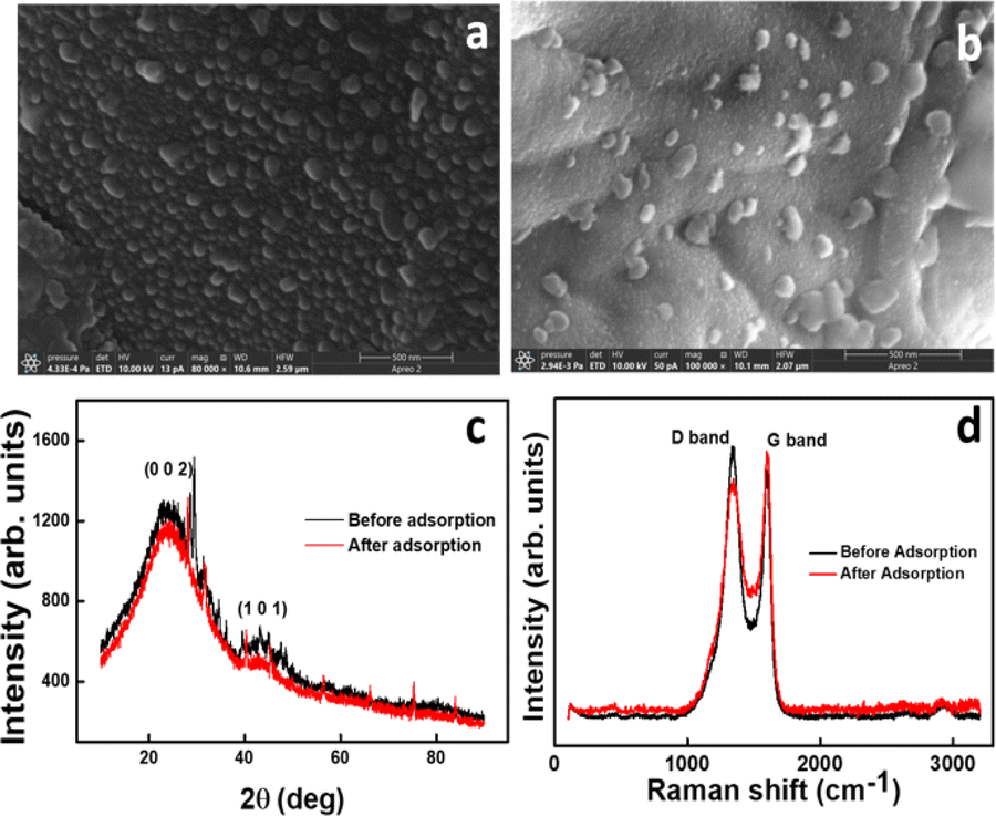 | ||
| Fig. 1 SEM image of GS-CNSs (a) before adsorption and (b) after dye adsorption; (c) XRD patterns and (d) Raman spectra of GS-CNSs before and after dye adsorption. | ||
C bonds in the G-band at 1600 cm−1 (Fig. 1d) indicates the graphitic nature of the resulting carbon nanospheres. In recent literature,37 this structure can be confirmed. The D-band peak to G-band peak intensity ratio is integralised to determine the degree of disorder in carbon (ID/IG). The ID/IG ratio of GS-CNSs was calculated to be 1.11 before adsorption and 0.89 after adsorption, which confirms the relatively high level of disorder structural defects of the synthesized nanospheres. The decrease in the ID/IG ratio might suggest that the dye molecules have adsorbed onto the surface of the nanoparticles and influenced their structural properties. This can happen through pi–pi stacking interactions, van der Waals forces, or other chemical interactions between the dye molecules and the GS-CNSs.
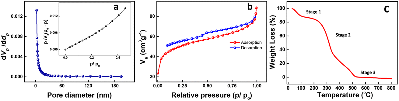 | ||
| Fig. 2 (a) BJH pore size distribution plot; (b) N2 adsorption–desorption isotherm for GS-CNSs; (c) TGA curve for raw precursors. | ||
CO stretching in the precursor. A peak at 2238 cm−1 shows an alkyne moiety in the precursor since it has cellulose and lignin. The peaks at 2021 cm−1 and 1912 cm−1 confirm the presence of the allene group. The peak at 1747 cm−1 confirms the CO stretching of the COOH group in hemicellulose and lignin present in the Arachis hypogaea powder. Due to lignin's conjugated carbonyl and the hemicelluloses in the groundnut, there is a stretching vibration at 1627 cm−1. The peak at 1435 cm−1 corresponds to the bending of C–H bonds in the methyl group of lignin.
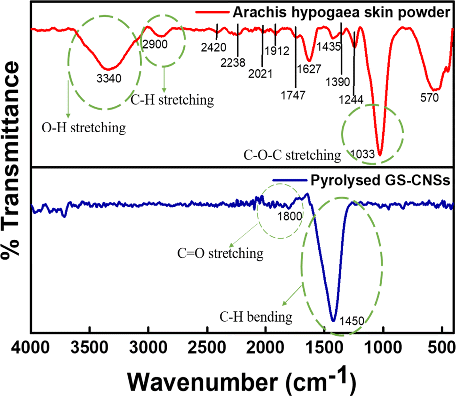 | ||
| Fig. 3 FTIR analysis of raw Arachis hypogaea skin powder and pyrolysed GS-CNSs. | ||
A characteristic feature of cellulose and hemicellulose is the symmetric deformation of C–H aldehyde bending, which is observable at 1390 cm−1. The 1244 cm−1 peak shows aromatic ester C–O stretching for a lignocellulosic nature. The peaks observed in the spectral range of 1000–1175 cm−1 and 900–550 cm−1 correspond to the stretching and non-symmetrical bending deformations involving C–O, C–C, and C–O–C bonds, as well as vibrations associated with C–H bonds, all of which are linked to the presence of cellulose and hemicellulose. Thus, FTIR data show that hemicellulose and lignocellulose are the main components of biowaste that can serve as carbon precursors in the production of highly ordered carbon nanospheres.18,36,38 After pyrolysis, the lignocellulosic group has been converted to carbon. The peak at 1800 cm−1 and 1450 cm−1 indicates the occurrence of CO stretching and C–H bending, respectively, showcasing that the precursor is pyrolysed.
Adsorption studies
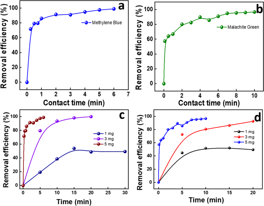 | ||
| Fig. 4 Effect of contact time for GS-CNSs on (a) MB and (b) MG dyes; effect of GS-CNS dosage on (c) MB and (d) MG dye adsorption. | ||
A comparative study is tabulated in Table 1 to demonstrate the effectiveness of the present work with respect to the previously conducted research and its results for cationic dye removal using carbon nanospheres as adsorbents.
| Dye | Dye conc. (μM) | CNS dosage (mg) | Adsorbent used & synthesis method | Removal efficiency (%) | Time (min) | Adsorption isotherm & kinetics | Ref |
|---|---|---|---|---|---|---|---|
| Malachite green | 10 | 1 | CNSs derived from oil palm leaves; pyrolysis at 1000 °C | 90 | 10 | Temkin isotherm; pseudo second order | 21 |
| Brilliant green | 10 | 1 | CNSs derived from oil palm leaves; pyrolysis at 1000 °C | 99 | 10 | Freundlich; pseudo second order | 21 |
| Malachite green | 10 | 1.5 | Garlic peel based mesoporous CNSs; pyrolysis at 1000 °C | 98.9 | 70 | Langmuir; pseudo second order | 20 |
| Methylene blue | 10 | 1.5 | Porous areca nut CNSs; pyrolysis at 1000 °C | 99 | 70 | Langmuir; pseudo second order | 18 |
| Methylene blue | 15.63 | 5 | Arachis hypogea skin derived CNSs; pyrolysis at 800 °C | 98.4 | 2 | R–P; pseudo second order | This work |
| 31.26 | 98.8 | 6 | |||||
| Malachite green | 13.70 | 5 | Arachis hypogea skin derived CNSs; pyrolysis at 800 °C | 97.4 | 2 | R–P; pseudo second order | This work |
| 27.40 | 96.6 | 10 |
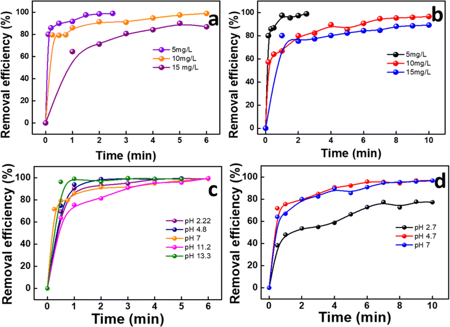
For MB, the removal efficiency was nearly 19, 80, and 98% for 1, 3, and 5 mg, respectively, by keeping the contact time at 5 min. Within 2 min, the efficiency was 91.3% for 5 mg adsorbent dosage. It is obvious that GS-CNSs can remove 99% of the methylene blue dye regardless of dosage; however, smaller dosages will require a longer time. Additionally, it's possible that greater dosages will result in more open adsorbent sites and surface area, which will make it easier for dye molecules to bind to the surface.40
The removal efficiency of MG for doses of 1, 3, and 5 mg is each depicted in Fig. 4d. For MG, the removal efficiency was 44, 74, and 85% for 1, 3, and 5 mg, respectively, by keeping the contact time at 5 min. For the 3 mg dosage, the removal efficiency crossed 92% after 20 min, whereas for the 5 mg dosage, it reached 96.6% in just 10 min. It must also be noted that the efficiency reached 80% within 2 min. Because of this, the dosage of 5 mg of GS-CNSs was decided upon for further investigations.
In addition, anionic dyes (such as congo red and indigo carmine) were tested in order to test the feasibility, but the removal efficiency was low even after a longer duration. Indigo carmine resulted in 12% removal in 5 minutes with a 3 mg dosage of GS-CNSs, whereas congo red showed 14% removal with the same GS-CNS dosage and time for 10 mg L−1 dye solution [refer to ESI Fig. S2† for dye removal studies for anionic dyes]. On the other hand, the cationic dyes MB and MG showed around 80% and 74% removal, with a 3 mg dosage of GS-CNSs in 5 minutes. This also contributes to the selectivity and surface charge on the carbon nanospheres, due to which a higher removal efficiency of cationic dyes can be observed than anionic dyes. Electrostatic stabilization plays a vital role here.
 | ||
| Fig. 5 Effect of (a) MB and (b) MG dye concentration on GS-CNSs; effect of pH on (c) MB and (d) MG dye adsorption with GS-CNSs. | ||
For MB, 5, 10, and 15 mg L−1 dye concentrations were used with 5 mg of adsorbent dosage for the experiment. For 5 mg L−1 (15.63 μM), the efficiency reached 98.4% in just 2 min. Similarly, for 10 mg L−1 (31.26 μM) and 15 mg L−1 (46.9 μM) concentrations, the efficiency was 98.8% and 86.81%, respectively in 6 min.
For MG, the 5 mg L−1 (13.70 μM) dye concentration showed 97.4% removal in merely 2 min, as depicted in Fig. 5b. When investigated for 10 mg L−1 (27.40 μM) and 15 mg L−1 (41.11 μM) dye concentrations, the dye removal efficiency was 96.61 and 89.24%, respectively, in 10 min. It is evident from the provided data for both the dyes that at lower concentrations, adsorption occurs at a higher pace, which is attributed to a smaller ratio of dye molecules to active adsorbent sites at lower concentrations. However, as the concentration increases, this ratio increases, leading to the saturation of the pores. During this saturation stage, the efficiency of dye removal decreases as dye molecules start to compete with each other for binding to the inner pores of the adsorbent.41 The critical variables influencing the retarding adsorption process are hence the optimal concentration and the growing ion competition that results in the saturation of active adsorption sites when dealing with higher initial concentrations. The reduced adsorption rate at higher concentrations can also be caused by the repulsion between adsorbed and remaining dye molecules.18,42
For MG dye, the efficiency was better at native and slightly acidic pH. Within 10 min of contact time, the efficiency of dye removal was found to be 96.6% at both pH 4.7 and pH 7 though it dropped to 77.18% at pH 2.72, as indicated in Fig. 5d. At a highly basic pH, the dye turns cyan and then colourless when saturated NaOH solution is added to the dye solution. Under low pH conditions, the abundance of readily available H+ ions can result in the protonation of electron-rich sites on the contaminants and/or CNSs. However, contaminants may compete with the OH− availability for basic pH for the sorbent's adsorption sites.45 Because MG is known to exist in cationic form in aqueous environments, it is attracted to negatively charged surfaces. The adsorption of MG was enhanced at higher pH values until 7 and subsequently reduced as the pH increased. This behaviour may be explained by the presence of extra negative charges on the nanoparticles' surfaces, which might strengthen their electrostatic interaction with the cationic dye MG.46 Due to the transformation of MG into protonated MG (MGH) under acidic pH conditions and into a carbinol base under basic pH conditions, the structural modifications of the molecule should be taken into consideration when removing the compound.47
Adsorption isotherms
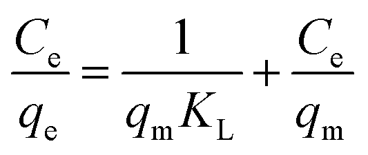
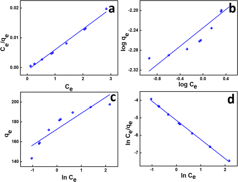
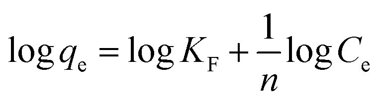
The relationship between the quantity of adsorbate adsorbed onto a particular adsorbent surface and the equilibrium concentration of the substrate while in contact with the adsorbent under constant temperature conditions is shown by adsorption isotherm curves.48,49 The Langmuir, Freundlich, Temkin, and Redlich–Peterson models were utilized in the current work to understand the adsorption mechanism and to linearly fit the batch equilibrium data.The following linear form can be used to express the Langmuir eqn (2):51
 | (2) |
This also implies the existence of homogeneous energy surface sites where adsorption occurs, as indicated by the initial increase in the curve and the achievement of the n-equilibrium point.49 As shown in Fig. 6a for methylene blue and Fig. 7a for malachite green, the graph is plotted with Ce/qe on the y-axis against Ce on the x-axis. From the plotted graph, the regression coefficient obtained for MB was 0.9905, and for MG, it was 0.9810, showing that MB adsorption best fits this isotherm. After calculations, the maximum adsorbent capacity for MB and MG was 1128.46 mg g−1 and 387.6 mg g−1, respectively. The RL parameter signifies that adsorption is non-reversible when RL = 0, linear when RL = 1, unfavourable when RL > 1, and favourable when RL falls within the range of 0 to 1. Here, for both MB and MG adsorption, the RL is favourable since the values obtained were 0.43 and 0.25, respectively.
 | ||
| Fig. 6 (a) Langmuir, (b) Freundlich, (c) Temkin, and (d) Redlich–Peterson isotherms of MB adsorption. | ||
 | ||
| Fig. 7 (a) Langmuir, (b) Freundlich, (c) Temkin, and (d) Redlich–Peterson isotherms of MG adsorption. | ||
The Langmuir model is grounded on the concept that the adsorption occurs through monolayer adsorption on a uniformly structured adsorbent surface. There are only a few identical adsorbate-binding sites. Additionally, adsorbed molecules do not come into contact with one another.
 | (3) |
 | (4) |
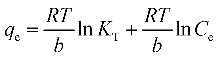
![[thin space (1/6-em)]](https://www.rsc.org/images/entities/char_2009.gif) Ce,20,54 as shown in Fig. 6c and 7c for MB and MG, respectively, and the values obtained from the graph are tabulated in Table 2. The Temkin graph indicates a regression coefficient fit of R2 = 0.8163 and 0.8905 for MB and MG, respectively. As a result, KT = 1.09764 L g−1 for MB. Similarly, BT = RT/b = 1.608 J mol−1 for MB and −0.03107 J mol−1 for MG show that the adsorption process is exothermic and physical in nature.
Ce,20,54 as shown in Fig. 6c and 7c for MB and MG, respectively, and the values obtained from the graph are tabulated in Table 2. The Temkin graph indicates a regression coefficient fit of R2 = 0.8163 and 0.8905 for MB and MG, respectively. As a result, KT = 1.09764 L g−1 for MB. Similarly, BT = RT/b = 1.608 J mol−1 for MB and −0.03107 J mol−1 for MG show that the adsorption process is exothermic and physical in nature.
| Isotherm models | Parameters | Methylene blue | Malachite green |
|---|---|---|---|
| Langmuir | q m (mg g−1) | 1128.46 | 387.6 |
| K L (L g−1) | 0.13 | 0.3 | |
| R L | 0.43 | 0.25 | |
| R 2 | 0.99054 | 0.98101 | |
| Freundlich | K F | 0.11 | 9.3 |
| n F | 10.79 | 5.41 | |
| R 2 | 0.78257 | 0.84777 | |
| Temkin | B T | 1.608 | −0.03107 |
| K T | 1.09764 | — | |
| R 2 | 0.81634 | 0.89053 | |
| Redlich–Peterson | B | −1.09269 | 2.72789 |
| A | 169.824 | 169.43 | |
| R 2 | 0.99807 | 0.99572 |
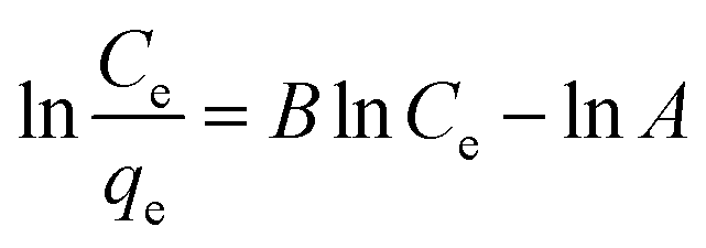 | (5) |
Ce/qevs. lnCe and the accompanying Fig. 6d and 7d for MB (R2 = 0.9980) and MG (R2 = 0.9980) dyes, the corresponding values are tabulated in Table 2, which best fit this isotherm. The Redlich–Peterson parameter was calculated to be −1.09269 for MB, whereas for MG, it was 2.72789. This isotherm model is versatile and can be applied to both homogeneous and heterogeneous systems. It captures adsorption equilibrium by exhibiting a linear relationship between a concentration in the numerator and an exponential function in the denominator, making it suitable for a broad spectrum of adsorbate concentrations.56
The experimental data show a strong fit for the Redlich–Peterson isotherm model, demonstrating its usefulness in predicting the adsorption behavior found in our study. The Redlich–Peterson model combines the Langmuir and Freundlich isotherm equations, providing a versatile method for characterizing adsorption on heterogeneous surfaces. It takes into account both monolayer and multilayer adsorption, allowing for differences in surface heterogeneity and adsorbate–adsorbent interactions. This complete model sheds light on the adsorption mechanisms that govern the interaction between GS-CNSs and the dye, helping in better understanding of the underlying processes that drive adsorption events.
Adsorption kinetics
Adsorption kinetics determines the rate of uptake of an adsorbate over time at a particular concentration and offers details on adsorbate diffusion into the pores, indicating a likely sorption process. It aids in comprehending ideal circumstances and how changes in various adsorption factors impact rates.48,57 The parameters and the corresponding values with the regression coefficient for the two kinetic models studied are tabulated in Table 3.| Kinetic models | Methylene blue | Malachite green | |
|---|---|---|---|
| PFO | k 1 (min−1) | 0.0465206 | 0.0467048 |
| q e (mg g−1) | 65.831 | 61.384 | |
| R 2 | 0.7805 | 0.77936 | |
| PSO | k 2 (g mg−1 min−1) | 0.000285 | 0.0001176 |
| q e (mg g−1) | 20063.6 | 19889.53 | |
| R 2 | 0.99876 | 0.99678 | |
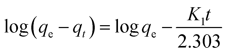
This model is given in eqn (6):58
 | (6) |
The amount of adsorbate in the adsorbent at equilibrium and time t (min), respectively, is represented by the variables qe and qt (mg g−1). k1 (min−1) is the pseudo-first-order rate constant in this equation. As a result of this characteristic, it is convenient to create a plot of log(qe − qt) on the y-axis and contact time t on the x-axis, which is displayed in Fig. 8a and c for MB (R2 = 0.7805) and MG (R2 = 0.77936), respectively, to test this isotherm. The values are shown in Table 3k1 values for MB were found to be 0.0465206 min−1, whereas for MG, it was 0.0467048 min−1.
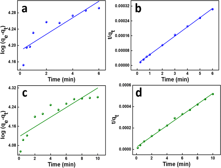 | ||
| Fig. 8 Pseudo first order kinetics for (a) MB and (c) MG; pseudo second order kinetics for (b) MB (d) MG adsorption. | ||
 | (7) |
This suggests that the rate-limiting step of the adsorption process involves the interaction between the adsorbate molecules and the active sites on the adsorbent surface. This implies that the adsorption is controlled by the availability of active sites and the chemical affinity between the adsorbate and adsorbent. This kinetics is indicative of a heterogeneous adsorbent surface, where different active sites have different affinities for the adsorbate.
In conclusion, the experimental data demonstrate a strong fit to the PSO kinetic model as seen from the data provided in Table 3, indicating the adsorption of dyes onto GS-CNSs. This model suggests that the rate-limiting step in the adsorption process involves chemisorption, wherein the interaction between dye molecules and GS-CNSs occurs through strong chemical bonding. The superior fit of the PSO model emphasizes the importance of chemical interactions in driving the adsorption behavior of GS-CNSs, providing useful insights for the design and optimization of adsorption processes in a variety of applications.
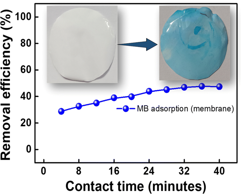 | ||
| Fig. 9 Removal efficiency of MB using a polysulfone membrane with GS-CNSs. | ||
A homogeneous membrane structure without significant irregularities or surface variations for pure polysulfone membranes can be observed when viewed under an optical profilometer. This suggests that the membrane fabrication process using NMP has resulted in a high-quality and well-formed polysulfone membrane with consistent surface morphology. [Refer to the ESI for Fig. S3 and S4†].
The 2D and 3D optical profilometer image of the polysulfone membrane incorporating GS-CNSs exhibits a modified surface topography compared to the pure polysulfone membrane. The image reveals the presence of carbon nanospheres dispersed throughout the membrane, leading to slight surface roughness and variations. This indicates the successful incorporation of the carbon nanospheres into the polysulfone matrix.
The optical profilometer image of the membrane after dye removal reveals significant changes in its surface topography. Prior to dye adsorption, the membrane exhibited a relatively smooth and uniform surface. However, following the adsorption process, distinct variations in the surface morphology are observed. The image displays irregularities, including localized depressions and roughness, indicating dye molecules being adsorbed onto the membrane surface. These alterations in the surface topography suggest that the dye molecules have effectively interacted and adhered to the membrane matrix. The optical profilometer image provides visual evidence of the successful dye removal process and highlights the membrane's ability to capture and retain cationic dyes from aqueous solutions.
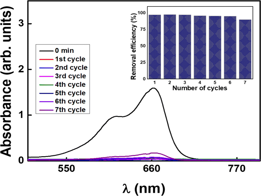 | ||
| Fig. 10 Absorbance spectra of treated MB dye samples in reusability study; the inset shows GS-CNSs showing the number of adsorption cycles. | ||
Conclusions and outlook
In the present study, Arachis hypogaea skin-derived carbon nanospheres are used as adsorbents to remove cationic dyes such as MB and MG in the aqueous solution. With merely 5 mg of adsorbent and 5 mg L−1 dye concentration, the removal efficiency reached approximately ∼98% for both dyes in just 2 min. Even for higher concentrations, the removal efficiency was around 98.8% for MB and 96.6% for MG in 6 and 10 min, respectively, with the same adsorbent dosage. The adsorption data were fitted to various kinetic and isothermal models to get insight into the adsorption mechanism and behavior. The pseudo-second-order kinetic model and the Redlich–Peterson model best fit the experimental data, showing that multi-layer adsorption and chemisorption were the primary adsorption mechanisms. The GS-CNSs also showed high surface area and high adsorption capacity for both dyes. This implies that these CNSs could be a promising alternative for wastewater treatment and dye removal mitigation. The use of groundnut skin as a precursor material for CNS synthesis also suggests a sustainable and cost-effective approach. The adsorption was a highly efficient and cost-effective method for the fast removal of cationic dyes. However, it is worth noting that the achieved removal efficiency of 48% using a membrane leaves room for further improvement in dye removal using a membrane system. Additional research is necessary to enhance the performance of the membrane system and achieve higher removal efficiencies. Factors such as membrane composition, surface modifications, and optimization of operating conditions should be explored to enhance the membrane's dye adsorption and removal capabilities. Further research in this direction to optimize the membrane system and understand the underlying mechanisms is in progress and will be reported elsewhere.Author contributions
Aman Sharma: conceptualization, investigation, methodology, data curation, formal analysis, writing—draft manuscript, writing—original draft, revision of the manuscript and editing, writing—review and editing. Jyothi Mannekote Shivanna: revision of the manuscript and editing, supervision, formal analysis, reviewing, and final approval of the manuscript to be published. Abdullah N. Alodhayb: revision of the manuscript and editing, reviewing, and final approval of the manuscript to be published. Gurumurthy Hegde: revision of the manuscript and editing, supervision, validation, formal analysis, reviewing, and final approval of the manuscript to be published.Conflicts of interest
There are no conflicts to declare.Acknowledgements
One of the authors, Gurumurthy Hegde, thanks the Centre for Research Projects, CHRIST (Deemed to be University) for providing financial support with grant number SMSS-2214. Another author Abdullah N. Alodhayb acknowledges Researchers Supporting Project number (RSP2024R304), King Saud University, Riyadh, Saudi Arabia.References
- F. Amalina, A. S. Abd Razak, S. Krishnan, A. W. Zularisam and M. Nasrullah, Cleaner Waste Syst., 2022, 3, 100051, DOI:10.1016/j.clwas.2022.100051.
- M. M. Hassan and C. M. Carr, Chemosphere, 2021, 265, 129087, DOI:10.1016/j.chemosphere.2020.129087.
- N. Kaya and Z. Y. Uzun, Biomass Convers. Biorefin., 2020, 11, 1067–1083, DOI:10.1007/s13399-020-01063-8.
- N. P. Raval, P. U. Shah and N. K. Shah, Appl. Water Sci., 2016, 7, 3407–3445, DOI:10.1007/s13201-016-0512-2.
- S. J. Culp, L. R. Blankenship, D. F. Kusewitt, D. R. Doerge, L. T. Mulligan and F. A. Beland, Chem.–Biol. Interact., 1999, 122, 153–170, DOI:10.1016/s0009-2797(99)00119-2.
- C. J. Cha, D. R. Doerge and C. E. Cerniglia, Appl. Environ. Microbiol., 2001, 67, 4358–4360, DOI:10.1128/AEM.67.9.4358-4360.2001.
- P. Ganguly, R. Sarkhel and P. Das, Surf. Interfaces, 2020, 20, 100616, DOI:10.1016/j.surfin.2020.100616.
- Y.-R. Lin, Y.-F. Hu, C.-Y. Huang, H.-T. Huang, Z.-H. Liao, A.-T. Lee, Y.-S. Wu and F.-H. Nan, Front. Environ. Sci., 2022, 10, 1–9, DOI:10.3389/fenvs.2022.906886.
- A. H. Jawad, R. Razuan, J. N. Appaturi and L. D. Wilson, Surf. Interfaces, 2019, 16, 76–84, DOI:10.1016/j.surfin.2019.04.012.
- H. Chandarana, P. Senthil Kumar, M. Seenuvasan and M. Anil Kumar, Chemosphere, 2021, 285, 131480, DOI:10.1016/j.chemosphere.2021.131480.
- A. Waheed, N. Baig, N. Ullah and W. Falath, J. Environ. Manage., 2021, 287, 112360, DOI:10.1016/j.jenvman.2021.112360.
- L. Soldatkina and M. Yanar, ChemEngineering, 2023, 7, 6, DOI:10.3390/chemengineering7010006.
- M. M. Aljumaily, N. S. Ali, A. E. Mahdi, H. M. Alayan, M. AlOmar, M. M. Hameed, B. Ismael, Q. F. Alsalhy, M. A. Alsaadi, H. S. Majdi and Z. B. Mohammed, Water, 2022, 14, 1396, DOI:10.3390/w14091396.
- A. T. Mansour, A. E. Alprol, K. M. Abualnaja, H. S. El-Beltagi, K. M. A. Ramadan and M. Ashour, Polymers, 2022, 14, 1735, DOI:10.3390/polym14071375.
- A. K. Badawi, M. Abd Elkodous and G. A. M. Ali, RSC Adv., 2021, 11, 36528–36553, 10.1039/D1RA06892J.
- N. U. M. Nizam, M. M. Hanafiah, E. Mahmoudi, A. A. Halim and A. W. Mohammad, Sci. Rep., 2021, 11, 1–17, DOI:10.1038/s41598-021-88084-z.
- I. Akkari, Z. Graba, N. Bezzi, M. M. Kaci, F. A. Merzeg, N. Bait, A. Ferhati, G. L. Dotto and Y. Benguerba, Environ. Sci. Pollut. Res. Int., 2023, 30, 3027–3044, DOI:10.1007/s11356-022-22402-4.
- D. Pathania, A. Araballi, F. Fernandes, J. M. Shivanna, G. Sriram, M. Kurkuri, G. Hegde and T. M. Aminabhavi, Environ. Res., 2023, 224, 115521, DOI:10.1016/j.envres.2023.115521.
- A. H. Jawad, A. S. Abdulhameed and M. S. Mastuli, J. Taibah Univ. SCI., 2020, 14, 305–313, DOI:10.1080/16583655.2020.1736767.
- D. Pathania, V. S. Bhat, J. Mannekote Shivanna, G. Sriram, M. Kurkuri and G. Hegde, Spectrochim. Acta, Part A, 2022, 276, 121197, DOI:10.1016/j.saa.2022.121197.
- B. Krishnappa, V. S. Bhat, V. Ancy, J. C. Joshi, S. Jyothi M, M. Naik and G. Hegde, Molecules, 2022, 27, 7017, DOI:10.3390/molecules27207017.
- B. Krishnappa, S. Saravu, J. M. Shivanna, M. Naik and G. Hegde, Environ. Sci. Pollut. Res., 2022, 29, 79067–79081, DOI:10.1007/s11356-022-21251-5.
- B. H. Hameed and M. I. El-Khaiary, J. Hazard. Mater., 2008, 155, 601–609, DOI:10.1016/j.jhazmat.2007.11.102.
- M. A. El-Nemr, N. M. Abdelmonem, I. M. A. Ismail, S. Ragab and A. El-Nemr, Desalin. Water Treat., 2020, 203, 403–431, DOI:10.5004/dwt.2020.26207.
- M. A. El-Nemr, N. M. Abdelmonem, I. M. A. Ismail, S. Ragab and A. El Nemr, Desalin. Water Treat., 2020, 203, 327–355, DOI:10.5004/dwt.2020.26190.
- E. F. D. Januário, T. B. Vidovix, L. A. de Araújo, L. Bergamasco Beltran, R. Bergamasco and A. M. S. Vieira, Environ. Technol., 2022, 43, 4315–4329, DOI:10.1080/09593330.2021.1946601.
- K. Sathya, H. Jayalakshmi, S. N. Reddy, M. V. Ratnam and D. Bandhu, Biomass Convers. Biorefine., 2023, 13(18), 1–13, DOI:10.1007/s13399-023-05213-6.
- A. Vakili, A. A. Zinatizadeh, Z. Rahimi, S. Zinadini, P. Mohammadi, S. Azizi, A. Karami and M. Abdulgader, J. Cleaner Prod., 2023, 382, 134899, DOI:10.1016/j.jclepro.2022.134899.
- S. Sunkar, P. Prakash, B. Dhandapani, O. Baigenzhenov, J. A. Kumar, V. Nachiyaar, S. Zolfaghari, S. Tejaswini and A. Hosseini-Bandegharaei, Environ. Res., 2023, 233, 116486, DOI:10.1016/j.envres.2023.116486.
- M. S. Jyothi, V. J. Angadi, T. V. Kanakalakshmi, M. Padaki, B. R. Geetha and K. Soontarapa, J. Polym. Environ., 2019, 27, 2408–2418, DOI:10.1007/s10924-019-01531-x.
- P. Wang, Q. Ma, D. Hu and L. Wang, Desalin. Water Treat., 2016, 57, 10261–10269, DOI:10.1080/19443994.2015.1033651.
- N. R. Putra, D. N. Rizkiyah, M. A. Che Yunus, A. H. Abdul Aziz, A. S. H. Md Yasir, I. Irianto, J. Jumakir, W. Waluyo, S. Suparwoto and L. Qomariyah, Molecules, 2023, 28, 4325, DOI:10.3390/molecules28114325.
- C. Lavanya, K. Soontarapa, M. S. Jyothi and R. Geetha Balakrishna, Sep. Purif. Technol., 2019, 211, 348–358, DOI:10.1016/j.seppur.2018.10.006.
- J. Deng, M. Li and Y. Wang, Green Chem., 2016, 18, 4824–4854, 10.1039/C6GC01172A.
- A. Nieto-Márquez, R. Romero, A. Romero and J. L. Valverde, J. Mater. Chem., 2011, 21, 1664–1672, 10.1039/C0JM01350A.
- S. Yallappa, D. R. Deepthi, S. Yashaswini, R. Hamsanandini, M. Chandraprasad, S. Ashok Kumar and G. Hegde, Nano-Struct. Nano-Objects, 2017, 12, 84–90, DOI:10.1016/j.nanoso.2017.09.009.
- S. Supriya, A. Divyashree, S. Yallappa and G. Hegde, Mater. Today, 2018, 5, 2907–2911, DOI:10.1016/j.matpr.2018.01.085.
- G. Hegde, S. A. Abdul Manaf, A. Kumar, G. A. M. Ali, K. F. Chong, Z. Ngaini and K. V. Sharma, ACS Sustainable Chem. Eng., 2015, 3, 2247–2253, DOI:10.1021/acssuschemeng.5b00517.
- M. Zhang, L. Chang, Y. Zhao and Z. Yu, Arabian J. Sci. Eng., 2019, 44, 111–121, DOI:10.1007/s13369-018-3258-3.
- J. Pal and M. K. Deb, Appl. Nanosci., 2013, 4, 967–978, DOI:10.1007/s13204-013-0277-y.
- A. T. Ojedokun and O. S. Bello, Appl. Water Sci., 2016, 7, 1965–1977, DOI:10.1007/s13201-015-0375-y.
- I. J. Idan, S. N. A. B. Jamil, L. C. Abdullah and T. S. Y. Choong, Int. J. Chem. Eng., 2017, 1–13, DOI:10.1155/2017/9792657.
- A. H. Jawad, A. S. Abdulhameed, L. D. Wilson, S. S. Syed-Hassan, Z. A. ALOthman and M. R. Khan, Chin. J. Chem. Eng., 2021, 32, 281–290, DOI:10.1016/j.cjche.2020.09.070.
- K. A. Tan, N. Morad and J. Q. Ooi, Int. J. Environ. Sci. Dev., 2016, 7, 724–728, DOI:10.18178/IJESD.2016.7.10.869.
- R. S. Almufarij, B. Y. Abdulkhair, M. Salih, H. Aldosari and N. W. Aldayel, Molecules, 2022, 27, 4577, DOI:10.3390/molecules27144577.
- A. S. Dehghan, M. Hassannezhad, M. Hosseini and M. R. Ganjali, J. Serb. Chem. Soc., 2019, 84, 701–712, DOI:10.2298/JSC181228038D.
- Y.-C. Lee, J.-Y. Kim and H.-J. Shin, Sep. Sci. Technol., 2013, 48, 1093–1101, DOI:10.1080/01496395.2012.723100.
- J. Wang and X. Guo, J. Hazard. Mater., 2020, 390, 122156, DOI:10.1016/j.jhazmat.2020.122156.
- M. Benjelloun, Y. Miyah, G. A. Evrendilek, F. Zerrouq and S. Lairini, Arabian J. Chem., 2021, 14, 103031, DOI:10.1016/j.arabjc.2021.103031.
- I. Langmuir, J. Am. Chem. Soc., 1918, 40, 1361–1403, DOI:10.1021/ja02242a004.
- N. Ayawei, A. N. Ebelegi and D. Wankasi, J. Chem., 2017, 11, 1–11, DOI:10.1155/2017/3039817.
- N. Ayawei, S. S. Angaye, D. Wankasi and E. D. Dikio, Open Phys. Chem. J., 2015, 5, 56–70, DOI:10.4236/ojpc.2015.53007.
- H. Shahbeig, N. Bagheri, S. Ghorbanian, A. Hallajisani and S. Pourkarimi, World J. Model. Simul., 2013, 9, 243–254 Search PubMed.
- B. R. Vergis, N. Kottam, R. Hari Krishna and B. M. Nagabhushana, Nano-Struct. Nano-Objects, 2019, 18, 100290, DOI:10.1016/j.nanoso.2019.100290.
- F. Brouers and T. J. Al-Musawi, J. Mol. Liq., 2015, 212, 46–51, DOI:10.1016/j.molliq.2015.08.054.
- F. Gimbert, N. Morin-Crini, F. Renault, P.-M. Badot and G. Crini, J. Hazard. Mater., 2008, 157, 34–46, DOI:10.1016/j.jhazmat.2007.12.072.
- J. Wang and X. Guo, Chemosphere, 2020, 258, 127279, DOI:10.1016/j.chemosphere.2020.127279.
- H. Moussout, H. Ahlafi, M. Aazza and H. Maghat, Karbala Int. J. Mod. Sci., 2018, 4, 244–254, DOI:10.1016/j.kijoms.2018.04.001.
- L. Meng, X. Zhang, Y. Tang, K. Su and J. Kong, Sci. Rep., 2015, 5, 7910, DOI:10.1038/srep07910.
- J. Jaafari, H. Barzanouni, S. Mazloomi, N. Amir Abadi Farahani, K. Sharafi, P. Soleimani and G. A. Haghighat, Int. J. Biol. Macromol., 2020, 164, 344–355, DOI:10.1016/j.ijbiomac.2020.07.042.
Footnote |
| † Electronic supplementary information (ESI) available. See DOI: https://doi.org/10.1039/d4na00254g |
| This journal is © The Royal Society of Chemistry 2024 |