
 Open Access Article
 This Open Access Article is licensed under a
 Creative Commons Attribution 3.0 Unported Licence
On the design of optimal computer experiments to model solvent effects on reaction kinetics†
Lingfeng
Gui
 a,
Alan
Armstrong
b,
Amparo
Galindo
a,
Fareed Bhasha
Sayyed
c,
Stanley P.
Kolis
d and
Claire S.
Adjiman
*a
a,
Alan
Armstrong
b,
Amparo
Galindo
a,
Fareed Bhasha
Sayyed
c,
Stanley P.
Kolis
d and
Claire S.
Adjiman
*a
aDepartment of Chemical Engineering, The Sargent Centre for Process Systems Engineering and Institute for Molecular Science and Engineering, Imperial College London, London, SW7 2AZ, UK. E-mail: c.adjiman@imperial.ac.uk
bDepartment of Chemistry and Institute for Molecular Science and Engineering, Imperial College London, Molecular Sciences Research Hub, White City Campus, London, W12 0BZ, UK
cSynthetic Molecule Design and Development, Eli Lilly Services India Pvt Ltd, Devarabeesanahalli, Bengaluru, 560103, India
dSynthetic Molecule Design and Development, Eli Lilly and Company, Lilly Corporate Center, Indianapolis, 46285, Indiana, USA
First published on 6th September 2024
Abstract
Developing an accurate predictive model of solvent effects on reaction kinetics is a challenging task, yet it can play an important role in process development. While first-principles or machine learning models are often compute- or data-intensive, simple surrogate models, such as multivariate linear or quadratic regression models, are useful when computational resources and data are scarce. The judicious choice of a small set of training data, i.e., a set of solvents in which quantum mechanical (QM) calculations of liquid-phase rate constants are to be performed, is critical to obtaining a reliable model. This is, however, made especially challenging by the highly irregular shape of the discrete space of possible experiments (solvent choices). In this work, we demonstrate that when choosing a set of computer experiments to generate training data, the D-optimality criterion value of the chosen set correlates well with the likelihood of achieving good model performance. With the Menshutkin reaction of pyridine and phenacyl bromide as a case study, this finding is further verified via the evaluation of the surrogate models regressed using D-optimal solvent sets generated from four distinct selection spaces. We also find that incorporating quadratic terms in the surrogate model and choosing the D-optimal solvent set from a selection space similar to the test set can significantly improve the accuracy of reaction rate constant predictions while using a small training dataset. Our approach holds promise for the use of statistical optimality criteria for other types of computer experiments, supporting the construction of surrogate models with reduced resource and data requirements.
Design, System, ApplicationIn molecular design, structure–property relationships are often evaluated with high-fidelity computationally-demanding models. Less expensive surrogate models, built from a set of computer experiments, can accelerate the search for better molecules. The reliability of the surrogate models, however, depends on how the training set is chosen. Computational tractability dictates a small number of data points should be used but this can lead to high uncertainty. We explore the impact of the experiment design strategy on model accuracy by investigating models of solvent effects on reaction rate constants. In this application, the high-fidelity model requires quantum mechanical calculations and the surrogate model is a multilinear relationship involving several solvent descriptors. It is especially challenging because the experimental inputs are discrete solvent choices. We identify the D-optimality criterion, a statistical metric commonly used for measuring the information content of a (physical) experimental design, as an indicator of good surrogate-model performance. These findings show that the application of the statistical experiment design criteria to the design of deterministic computer experiments (with systematic errors only) is a promising strategy. This approach could potentially be used in any data-deficient context where limited computational resources need to be leveraged to perform surrogate-based optimisation for molecular design. |
1 Introduction
1.1 Modelling solvent effects on reaction kinetics
A judicious choice of solvent for a liquid-phase reaction can improve reaction outcomes via the promotion of favourable reaction kinetics,1 a principle which is utilised in reaction planning and optimisation for the production of many chemicals, including bio-fuels,2,3 ionic liquids,4 pharmaceuticals,5 polymers,6 and others. However, solvent screening and selection via experiments is labour- and resource-intensive. In addition, repetitive measurements of liquid-phase reaction kinetics can be tedious and prone to human errors due to the complexity of the task, which typically involves reaction preparation, reaction monitoring, data analysis, etc. Emerging high-throughput experimentation (HTE) technologies can greatly speed up the solvent screening process. As an example, Li et al.7 completed a screening of 48 catalyst/solvent combinations for an aza-Michael reaction within a week via their high-throughput kinetic platform, significantly accelerating the development of a mechanistic model. Unfortunately, as of now, the barrier to entry associated with HTE technologies remains high due to the need for specialised equipment and operators. Even with access to HTE, the number of solvents that can be explored at any one time is limited by the dispensing capacity of the equipment. Furthermore, developing a successful HTE protocol and testing it can take a considerable amount of time, often spanning several months. In early stages, it may thus be beneficial to resort to computational methods to evaluate solvent effects on reaction kinetics in silico as a preliminary screening approach to guide experimental work with the aim to shorten development time and reduce the use of experimental materials.In general, there are two categories of methods for modelling solvent effects on reaction kinetics: first-principles methods and data-driven methods. First-principles methods are based on the fundamental theories of quantum mechanics and statistical mechanics that govern chemical reactions.8,9 Although their performance varies with the specific reactions and solvents examined, recent studies9,10 have demonstrated that they can achieve high predictive accuracy especially for relative rate constants, with mean absolute deviations as low as 0.9/0.27 in the base-10 logarithm of the predicted absolute/relative rate constant.9 Additionally, they can also provide physical insights into the reaction of interest. Nevertheless, these methods can be computationally expensive and require the use of high-performance computing facilities, especially for large molecular systems. In addition, a significant amount of specialised knowledge is required to perform these calculations in a correct manner. Machine learning (ML) methods, on the other hand, have emerged as a promising class of data-driven methods for the prediction of various reaction properties, including activation barriers and reaction rates.11 By fitting generalised mathematical models, e.g., artificial neural networks (ANNs), random forests (RFs), Gaussian process regression (GPR) models and many others, to a large amount of training data (up to 105 or more depending on the model type and number of parameters12), fast and accurate interpolation can be achieved by non-experts at a low computational cost. However, the high efficiency of these models comes at the cost of a large amount of training data, which are not always available and may be challenging to generate automatically due to the relatively high likelihood of numerical failure in applying first-principles models to varying reaction conditions. Given this context, it is desirable to develop data-sparse methods for the modelling of solvent effects on reaction kinetics, such as multivariate linear regression (MLR) models. A MLR model is distinguished by its mathematical simplicity and prerequisite for a smaller training data set than most machine learning models, thus providing unique advantages for quickly developing liquid-phase kinetics models. Additionally, they are often more computationally efficient and less prone to overfitting compared to more sophisticated ML models.13
One example of an MLR model commonly used in physical organic chemistry and chemometrics is the solvatochromic equation, a linear free energy relationship (LFER) that correlates a free energy-related quantity with a set of solvent properties that have been chosen empirically. The success of solvatochromic equations has been demonstrated for the prediction of various physicochemical properties, such as free energies of transfer of ions,14 gas/liquid partition coefficients,15 organic solvent/water partition coefficients,16,17 equilibrium constants18,19 and rate constants.20–22 The wide use of solvatochromic equations is partially due to the availability of a large collection of experimental solvatochromic parameters in the literature,17,23,24 with more being measured.25 In addition, computational methods have also been developed to estimate unknown solvatochromic parameters of pure solvents21,26 or selected solvent mixtures.27 In particular, group contribution methods21,26 for the estimation of solvatochromic parameters are useful for the assessment or design of solvent molecules for which no measured values are available.21,22
The usefulness of MLR models in enabling judicious solvent choices has previously been demonstrated in the literature. Struebing et al.22 used a solvatochromic equation as a surrogate model to substitute computationally-expensive quantum mechanical (QM) calculations. They performed surrogate-based optimisation to find solvents that can accelerate the Menshutkin reaction of pyridine and phenacyl bromide by maximising the rate constant as a function of solvent choice. To develop the surrogate model, training data were generated by performing computer experiments, i.e., QM calculations, in an initial set of six solvents chosen by chemical intuition. The surrogate model was then improved with the inclusion of new data generated during the course of the optimisation. The final optimal solvent was proven experimentally to increase the reaction rate constant by 40% compared to the best initial solvent. Despite this success in finding a solvent with enhanced performance, the accuracy of the solvatochromic equation was not verified over a larger solvent space and this may call the validity of the equation into question. Indeed, Williams and Cremaschi28 have pointed out that the sampling method, i.e., the method for determining which computer experiments to perform, can influence the quality of the solutions obtained from surrogate-based optimisation, especially when the number of training data points is small. Choosing initial computer experiments by chemical intuition, albeit common practice, may induce large inconsistencies in the performance of the resulting model, at best requiring more computer experiments to improve the model and at worst resulting in a poorer solution from surrogate-based optimisation. Therefore, the judicious design of computer experiments to generate a set of training data that is as informative as possible is important for reducing the use of resources and time and for improving model performance in a context of data scarcity. The question arises as to how one can systematically design computer experiments to generate a training data set of a given size such that the likelihood of obtaining an accurate surrogate model is improved or even maximised.
1.2 Design of physical and computer experiments
In physical experiments, a large source of uncertainty comes from the random errors in measurements. These errors propagate to the model parameters in the process of regression/fitting and cause errors in prediction. Assuming the chosen model adequately describes the target property to be predicted, the primary goal of design of experiments (DoE) is to generate a training set that minimises the uncertainties in the parameter estimation and/or the predicted properties.29 DoE techniques, including standard designs and optimal designs, are commonly used to mitigate the impact of random errors.30 Standard designs, such as factorial designs, are pre-defined designs with fixed patterns, irrespective of the statistical model used. By contrast, optimal designs are derived from model-based design of experiments (MBDoE) methods and are generated by maximising/minimising a specific statistical criterion with respect to a pre-specified statistical model.31 Optimal designs are especially useful when the shape of the selection space, i.e., the set of possible experiments, is irregular.30 Many optimal design methods reply on the assumption of normally distributed random errors with constant nonzero variance. For example, the D-optimality criterion, one of the most commonly used MBDoE statistical criteria, maximises the determinant of the Fisher information matrix30 with the aim to generate a model with minimal uncertainties in the estimated parameters. There also exist other widely applied statistical criteria, such as the A-optimality criterion,32 the I-optimality criterion33 and the condition number criterion.34,35 Of particular interest here, there have been several precedents34–36 in which an optimal design approach was used to generate a set of solvents in which reaction rate constants were measured experimentally and used to train a solvatochromic equation to quantify solvent effects on the rate constants of chemical reactions, including the solvolysis of tert-butyl chloride,34,36 the amination of ethyl trichloroacetate with ammonia35 and the Menshutkin reaction of tripropylamine and methyl iodide.36Beyond physical experiments, one can also generate training data from computer experiments. A computer experiment can be formally defined as a trial where a set of inputs (or configurations) is given to a computer model that generates a corresponding set of outputs. The purpose of performing computer experiments is often to derive a surrogate model in place of an original model that is too expensive to be used for certain activities such as optimisation.37,38 When the capability for performing computer experiments is limited, the choice of configurations is as important as for physical experiments. Common methods for the design of computer experiments include Monte Carlo sampling, Latin hypercube design and maximum entropy sampling.39 Here we focus on some published works on the design of computer experiments for the construction of surrogate models of reaction kinetics or kinetics-related quantities.
There have been several endeavours focused on the use of a space-filling objective for the design of computer experiments,40 or on the use of a Box–Behnken response surface design.41 Space-filling methods aim to achieve comprehensive coverage of the “experimental” or selection space and to minimise the unexplored gaps as much as possible such that the identified computer experiments can represent the whole input selection space. In this context, Xing et al.41 developed response surface models (RSMs) to replace the computationally expensive mechanistic models of two CO2 capture reactors. They used a Box–Behnken design to generate 46 sets of input variables from which three objective functions, including the CO2 capture rate, were calculated using the mechanistic models. The generated data were used to train the RSMs, resulting in a prediction R2 of 0.9411 and a RMSE of 0.1463 kg h−1 for the CO2 capture rate in a trickle bed reactor and a prediction R2 of 0.9999 and a RMSE of 0.0038 kg h−1 for a packed bubble column reactor. The RSMs were later incorporated into extended adaptive hybrid functions (E-AHF) to be used for chemical reactor optimisation. The effectiveness of using the Box–Behnken design was not discussed in detail. Lee et al.42 argued that Box–Behnken designs and other classical RSM designs cannot adequately cover the whole sampling space, thus making it difficult to capture highly nonlinear relationship. Instead, they suggested that space-filling methods, such as Latin hypercube sampling (LHS), can span a broader space to capture the mechanistic complexity of the process. They used LHS in the context of the continuous manufacture of active pharmaceutical ingredients (APIs), in which reaction kinetics play a critical role, to generate 2500 sample points at which simulations of the manufacturing process were run. The generated data were used to train a thin-plate spline model43 to serve as a surrogate model. Adjusted R2 values greater than 0.995 were obtained for all their models. Miriyala et al.44 showed that Sobol' sampling can achieve a level of space-filling comparable to the LHS method. A Sobol' sequence was used to sample the input space of a group of ordinary differential equations that describe the kinetics of the polyvinyl acetate reaction network. An artificial neural network (ANN) was trained using the generated data and found to require fewer training data (80 data points) compared to a GPR model (148 data points) of comparable accuracy and to provide higher computational efficiency. Williams and Cremaschi28 studied the choice of space-filling methods and the effect of the number of training data points on the performance of surface approximation and surrogate-based optimisation for 8 types of surrogate models. They evaluated LHS, Sobol' sequence sampling and Halton sequence sampling but did not report a significant impact of the choice of sampling method on the quality of the surface approximation. Nonetheless, based on the evaluation of 127 test functions with varying numbers of inputs, they found that for surrogate-based optimisation using random forests (RFs) and radial basis function networks, a Sobol' sequence generally leads to better estimates of the global minima of the test functions, especially when the number of training data is small (50 data points).
These examples demonstrate how computer experiments can be designed to fulfill the objective of space-filling, i.e., exploration of the input selection space. Exploitation, i.e., sampling regions that have been previously identified as promising in order to refine predictions, is another objective that often needs to be balanced against exploration when designing (computer) experiments. Exploitation is usually achieved by an adaptive design approach as the importance of potential sample points needs to be evaluated before the next sampling step is taken.
For example, Bracconi and Maestri45 proposed an adaptive design approach to construct a surrogate model based on Extra-Trees, a revised version of RF, for computationally expensive first-principles kinetic models in the context of the computational fluid dynamics simulation of chemical reactors. After training with an initial set of evenly distributed data points, the model was iteratively updated with a new sample point per iteration, chosen based on the quantified importance of each direction in the input space and the rate of variation of the output function value in that space. Using this approach, similar accuracies can be achieved with 60% to 80% fewer data points compared to an evenly distributed grid. In a similar context of training machine learning models with computer experiments, Eason and Cremaschi46 compared three computer experiment design methods for developing a model of CO2 capture cost. The methods considered include a pure space-filling sampling method that maintains a Latin hypercube design every time the number of sampling points is increased (incremental Latin hypercube sampling or i-LHS), a pure adaptive sampling algorithm in which points with least variance estimates are sampled, and a mixed adaptive sampling algorithm that accounts for both space-filling and uncertainty at the sample point in a weighted-sum fashion. They used a Latin hypercube design with 60 data points as the initial training data and found that when using diethanolamine as the carbon capture solvent, the mixed adaptive sampling algorithm only needs 270 total simulation runs (vs. 891 using i-LHS) and leads to a CO2 capture cost of $46.46 per ton, which is similar to the result obtained through the i-LHS approach ($46.21 per ton). As demonstrated in these examples, the required number of training data points can be lowered via the exploitation of more interesting areas of the selection/input space. When a good balance between exploration and exploitation is achieved, e.g., using the mixed adaptive sampling algorithm, even better performance may be observed. However, even an adaptive design approach cannot bypass the selection of an initial set of computer experiments, a decision which can have a large influence on subsequent adaptive sampling steps. In addition, one advantage of the one-time design approach over the adaptive design approach is that the former allows the full use of parallel computing while the latter requires sequential computing to determine and perform each new (set of) computer experiment(s), which may result in larger wall times despite the use of fewer data points.
When the input space consists of reaction solvents, the discrete nature of the solvent choice makes the application of some of the aforementioned methods more challenging. In previous work on solvent design using computer experiments,21,22 the common practice of choosing the initial set of solvents based on the chemical intuition of an expert chemist was adopted, but this does not provide any assurance on the quality of the resulting surrogate model. Instead, it is possible to project the discrete space of solvents into a latent continuous space of solvent descriptors or properties. For example, Zhou et al.47 projected the solvent space into the descriptor space of four principal components derived from the integrated areas of twelve solvent σ-potential segments calculated by COSMO-RS.48 They then applied partitional clustering49 to the principal components to classify solvents into eight classes. Diversity in the training dataset was achieved by selecting representative solvent(s) from different classes. Since solvent properties depend on molecular structure through highly complex interactions that are described at a fundamental level by quantum mechanics and statistical mechanics, the latent space of solvent properties is irregular, a situation which is challenging for space-filling methods and where MBDoE methods may be better suited.34 However, it is unclear whether MBDoE methods that are suitable for the optimal design of physical experiments can also be used to design computer experiments. While some computer experiments entail inherent uncertainties (e.g., molecular dynamics50), thus requiring multiple samples to obtain statistically valid results as in physical experiments, many other types of computer experiments are deterministic, which violates the assumption of normally distributed random errors that underpins many optimality criteria. Consequently, the application of MBDoE methods to computer experiments lacks a firm theoretical basis.51 Nevertheless, we recently showed that the D-optimal design of computer experiments can lead to an initial set of solvents that is superior to that derived from chemical intuition when attempting to build a surrogate model of the effect of solvent structure (properties) on liquid-phase rate constants.52 This MBDoE approach to the design of computer experiments generally leads to more accurate models and fewer iterations to complete surrogate-based optimisation, showing promise for the application of the D-optimality criterion to the design of computer experiments in an irregular input space.
In the current paper, we extend our previous study52 by systematically investigating the relationship between the D-optimality criterion values of a set of computer experiments and the performance of the resulting surrogate model. Four distinct selection spaces (also referred to as input spaces or sample spaces) for the computer experiments, i.e., four sets of possible solvents, are considered for the identification of D-optimal training datasets. These selection spaces differ from one another in the total number of solvents, in how the solvents are constructed (e.g., from a database of solvents from atom groups or by using a continuous relaxation of the space of solvents) and in how the solvents are projected onto the continuous latent space (e.g., using experimental property values or using group contribution methods). We investigate these differences via statistical analysis before considering the quality of the models that can be generated from each space. Specifically for each selection space, one D-optimal solvent set is identified. Rate constants for the Menshutkin reaction between pyridine and phenacyl bromide in these D-optimal solvents are then calculated using a QM method. The data thus generated are used to train a LFER, i.e., a multilinear surrogate model. The performance of each model is analysed quantitatively and qualitatively through comparisons with QM rate constants and with solvent rankings. We also explore the possibility of further improving the surrogate model by assessing three factors that may affect model performance: a) the number of training solvents in the D-optimal set, b) the incorporation of quadratic terms in the surrogate model and c) the similarity of the solvent selection space to the testing data set.
2 Methods
The method developed in this work aims to select an optimal set of computer experiments (evaluations of a high-fidelity, computationally demanding model) that can be used to develop an accurate surrogate (inexpensive) model of solvent effects on the rate constant of a given reaction. The overall methodology is illustrated in Fig. 1. In step 1, the surrogate model is chosen to be a linear or quadratic free energy relationship, as described in section 2.1. Based on this choice and the desired number, p, of computer experiments (solvents for which the rate constant can be evaluated), a Fisher information matrix is constructed, where row i corresponds to a solvent, where i = 1, …, p. The aim of the proposed method is thus to determine which specific solvents should be used to fill the rows of the matrix. In step 2, discussed in section 2.2, the space of possible computer experiments (i.e., a large set of l solvents, l > p), or selection space, is defined. In step 3, the identification of p solvents from the selection space is based on maximising the D-optimality criterion (the determinant of the Fisher information matrix), thereby generating the D-optimal design. Depending on the nature of the selection space, Fedorov's algorithm or a nonlinear programming approach is employed, as discussed in section 2.3. The p computer experiments are carried out in step 4, as a set of quantum mechanical calculations that yield rate constants, as described in section 2.4. The data thus generated are used in step 5 to train a surrogate model, using a standard linear regression solver. Finally, in step 6, several model performance indicators, described in section 2.5, are used to evaluate the ability of the surrogate models to capture the predictions of the quantum mechanical model.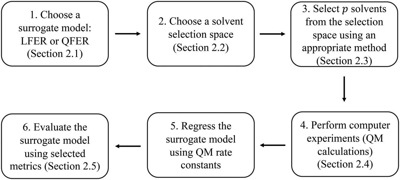 | ||
| Fig. 1 The model development procedure adopted in this work. | ||
2.1 Regression models
We use a new LFER based on the solvent descriptors tabulated in the Minnesota solvent descriptor database53 (https://comp.chem.umn.edu/solvation/mnsddb.pdf):ln![[thin space (1/6-em)]](https://www.rsc.org/images/entities/char_2009.gif) kL,LFER = β0 + β1A + β2B + β3n2 + β4γ + β5ε + β6ϕ + β7ψ, kL,LFER = β0 + β1A + β2B + β3n2 + β4γ + β5ε + β6ϕ + β7ψ, | (1) |
| lnkL,QFER = β0 + β1A + β2B + β3n2 + β4γ + β5ε + β6ϕ + β7ψ + β8A2 + β9B2 + β10γ2 + β11ε2, | (2) |
 | (3) |
| xTi = [1 Ai Bi n2i γi εi ϕi ψi]. | (4) |
| xTi = [1 Ai Bi n2i γi εi ϕi ψi A2i B2i γ2i ε2i]. | (5) |
![[scr I, script letter I]](https://www.rsc.org/images/entities/char_e143.gif) = F*TF*,30 can then be found by solving:
= F*TF*,30 can then be found by solving: | (6) |
2.2 MBDoE solvent selection spaces and test set
In this section, we define the selection spaces from which the D-optimal solvent sets are generated. Let F be a l × q matrix representing the MBDoE solvent selection space where l is the number of solvents in the space. The structure of F is similar to that of F*: column 1 of F is the identity vector and each of the other elements Fm,j, m = 1, …, l and j = 2, …, q, represents the (j − 1)th descriptor of candidate solvent m. The MBDoE problem can be stated as the selection of p rows of F to construct an optimal p × q matrix, F*,D, that maximises the D-optimality criterion.Four selection spaces are considered in our work, resulting in four MBDoE problems. Selection space 1 (SS1) is composed of all solvents in the Minnesota solvent descriptor database53 for which the experimental descriptor values are tabulated and ready to be used (excluding water).
We use the solvents in the CAMD design space in Grant et al.55 and Gui et al.56 as selection space 2 (SS2). The solvents in the CAMD design space include all the chemically feasible molecules that can be constructed from a pre-defined list of atom groups with specified physical and design constraints. These constraints can be found in the GAMS file provided in the Zenodo online repository. This CAMD design space also includes four common solvents that are described by “single-molecule” groups, i.e., chloroform, acetonitrile, N-methylformamide and dimethyl sulfoxide. Group contribution methods are used to calculate the descriptors of all these molecules. A more detailed discussion on the construction of this CAMD design space can be found in Grant et al.55 and Gui et al.56 The atom groups used to generate solvents and all the solvents in SS2 can be found in the GAMS code and Excel sheet provided in the Zenodo online repository.
Selection space 3 (SS3) is also constructed using chemically feasible molecules assembled from atom groups, but all the physical and design constraints are removed except a set of bounds on the descriptors to ensure their values are within reasonable ranges. The constraints removed include the bounds on melting point, boiling point, flash point, octanol/water partition coefficient and oral rat median lethal dose. Additional atom groups previously deactivated in SS2 due to potential reactivity in the Menshutkin reaction are activated in SS3. The bounds for the descriptors are established based on their maximum and minimum values in SS1 and SS2, as given in the GAMS code provided in the Zenodo online repository. The four single-molecule groups in SS2 are not included in SS3. Despite the risk of generating molecules that cannot physically exist as a liquid solvent (for example, ethane, 2 × CH3, is in SS3 but it is a gas at the room temperature and cannot be used as a liquid solvent under common processing conditions), this approach can greatly expand the selection space without being constrained by the availability of experimental solvent property values, bringing the potential of further increasing the D-optimality criterion values.
Even more radically, selection space 4 (SS4) is constructed with solvents solely defined by the set of bounds (same as those used for constructing SS3) on the continuous descriptors, without any explicit link to chemical structure, which produces an infinite number of “molecules” in SS4. The computer experiments can be performed for these hypothetical solvents but this approach can result in “solvents” that have unphysical combinations of descriptors (e.g., zero acidity and basicity and a high dielectric). Nevertheless, it also allows a full exploration of the high-fidelity model.
2.3 MBDoE solution methods
The strategy used to identify a D-optimal set of solvents depends on the selection space used and two approaches are described in this section. combinations. This MINLP formulation is given in section 2.1.2 of Gui et al.56 However, due to the large size of l (hundreds to thousands of solvents), the resulting MINLP cannot be solved in a tractable computational time. Instead, we use Fedorov's algorithm,57 one of the most common solution methods for the selection of experiments to maximise D-optimality. It is an iterative approach based on the exchange of selected experiments with candidate experiments in a pre-defined candidate list. Although Fedorov's algorithm cannot guarantee local or global optimality, we find that in most cases, it can identify better solutions with larger D-optimality criterion values than those generated from an optimisation-based approach using a local solver, such as DICOPT58 and SBB.59 Every time Fedorov's algorithm is used to generate a specified number of MBDoE solvents, three randomly-generated initial guesses are used, and the best solution generated among the three is considered as D-optimal. We observe that very often multiple initial guesses lead to the same solution.
In this section, a brief introduction to Fedorov's algorithm is given. A detailed discussion of its implementation can be found in the tutorial article by de Aguiar et al.57 Fedorov's algorithm starts with an initial guess of the F* matrix, and we denote the corresponding initial information matrix as (F*TF*)0. In the first iteration of Fedorov's algorithm, one of the initially-selected solvents is exchanged with another candidate solvent in the selection space F, i.e., row i of the initial F* matrix (xi) with row m of the selection space matrix F (xm). Then the updated information matrix is:
| (F*TF*)1 = (F*TF*)0 − (xixTi) + (xmxTm). | (7) |
| |F*TF*|1 = |F*TF*|0(1 + Δ(xi,xm)), | (8) |
| Δ(xi,xm) = d(xm) − d(xi) − [d(xi)d(xm) − d2(xi,xm)], | (9) |
| d(xi) = xTi(F*TF*)−10xi, | (10) |
| d(xm) = xTm(F*TF*)−10xm, | (11) |
| d(xi,xm) = xTi(F*TF*)−10xm. | (12) |
: | (13) |
, which is difficult to formulate directly in an optimisation framework. Instead, the LDL decomposition of the information matrix = LDLT is used.60L is a lower unit triangular matrix and D is a diagonal matrix. L and D can be calculated as below:61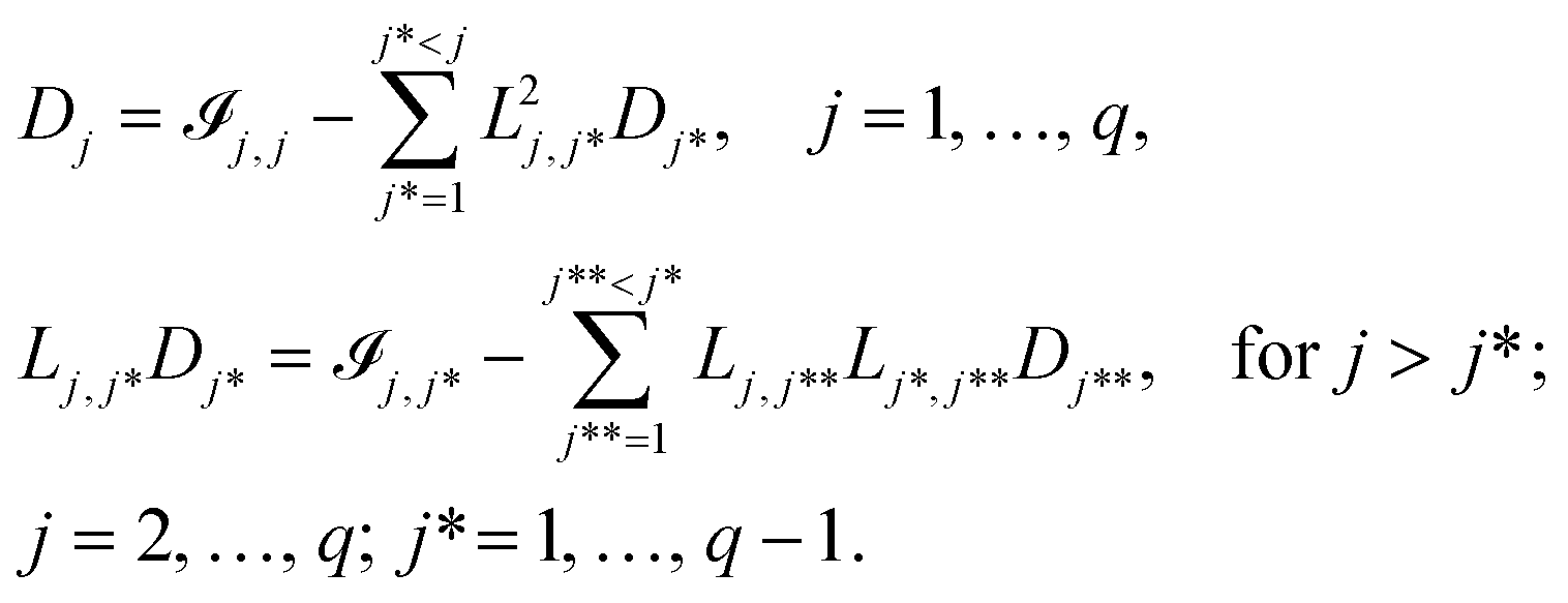 | (14) |
, i.e., the objective function of the NLP problem OF, can be expressed as,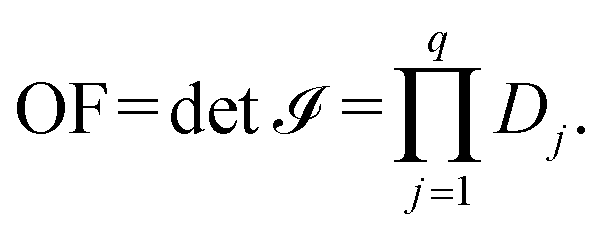 | (15) |
2.4 QM calculations of the liquid-phase reaction rate constants
The QM liquid-phase rate constant kL,QMi in solvent i is calculated using transition-state theory62,63 as: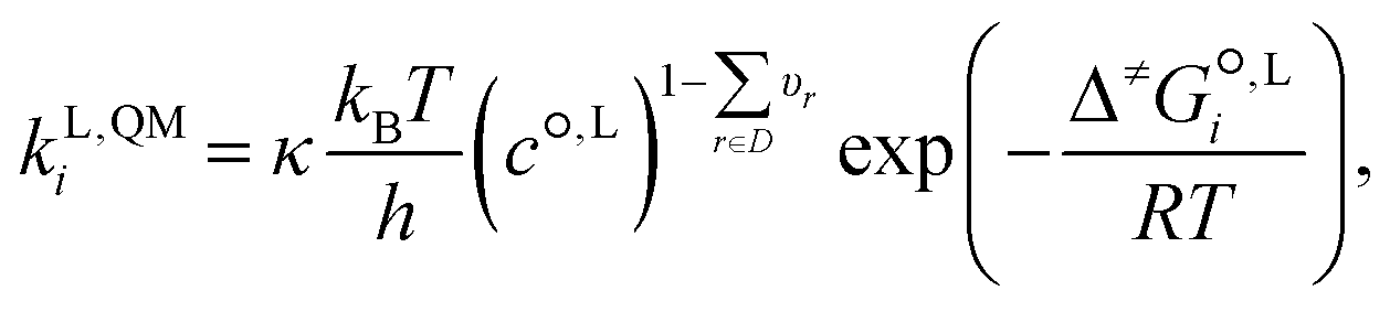 | (16) |
 is the liquid-phase activation Gibbs free energy of the reaction in solvent i, κ is the Wigner tunnelling correction factor,64kB is the Boltzmann constant, T = 298.15 K is the temperature, h is the Planck constant, R is the ideal gas constant, c°,L is the molar concentration at the standard state, D is the set of reactant(s) and υr is the stoichiometric coefficient of reactant r ∈ D.
We employ a thermodynamic cycle (TC) approach8 to calculate the liquid-phase activation Gibbs free energy  for the conversion from the reactant(s) to the transition state in solvent i,
 | (17) |
 is the solvation free energy of the transition state in solvent i,
  is the solvation free energy of reactant r in solvent i and P0 is the reference pressure. The last term is the standard-state correction, which is required to account for moving from the gas-phase standard state defined by T = 298.15 K and P0 = 1 atm to the solution-phase standard state of 1 mol L−1. The solvation free energies are calculated using the SMD solvation model54 at M06-2X/6-31+G(d)65 with the geometries in the gas and liquid phases optimised at the same level of theory in their respective phase. The ideal gas-phase activation Gibbs free energy is calculated using the composite method G3MP266 with the gas-phase M06-2X/6-31+G(d)65 geometry. All the calculations are performed in the Gaussian 16 software.67 Further details of how each term is calculated can be found in section 2.2.1 of Gui et al.56
2.5 Model performance indicators
In this work, the surrogate model is used in order to replace computationally expensive QM calculations of liquid-phase reaction rate constants. It is therefore important to test the reliability and accuracy of the surrogate models constructed. For this purpose, a test set is generated by calculating values of kL,QMi for all solvents in SS2. All values obtained can be found in the Excel sheet provided in the Zenodo online repository. One of the factors we consider for the regression of the surrogate models is the similarity of the MBDoE selection space to the test set. SS2, being identical to the test set, is the selection space with the greatest similarity to the test set. Furthermore, three metrics are used to assess the performance of the surrogate models constructed throughout this work against quantum mechanical calculations: the mean absolute deviation (MAD), Spearman's rank correlation (RC) and the root mean squared deviation of the top 20 solvent rankings (RMSDR-20).The first metric, MAD, measures the model accuracy in predicting the natural logarithms of the rate constant values for all solvents in the test set (SS2) and can be calculated as
 | (18) |
The second metric, RC, measures the model accuracy in predicting correct solvent rankings in terms of the rate constants for all solvents in the test set (where rank 1 corresponds to the largest rate constant) and it can be calculated as
 | (19) |
Finally, we examine the performance of the models in predicting the behaviour of the solvents with the largest reaction rate constants, as those are often the most relevant solvents. Because of this is a much smaller subset of solvents, a different ranking metric is defined. The final metric, the root mean squared deviation of the top 20 solvent rankings (RMSDR-20), is used to indicate the model performance for the 20 solvents that lead to the largest lnkL,QM, as these are the solvents that are typically most relevant in viewing the model,22 and it is calculated as
 | (20) |
kL,QM. RMSDR-20 is used instead of Spearman's rank correlation for this solvent subset because, when the ranges of Rsurrogatel and RQMl are different, RC (eqn (19)) is no longer on a scale from 0 to 1. Thus, the statistical meaning of RC is not straightforward to interpret.
3 Results and discussion
3.1 Relationship between model performance and D-optimality criterion values
First, the relationship between the performance of the LFER surrogate model and the D-optimality criterion values is investigated systematically. In physical experiments where measurements are subject to normally distributed random errors, the D-optimality criterion can be interpreted geometrically as the volume of the joint confidence region of the model parameters. A larger D-optimality criterion value is thus associated to provide greater chance of obtaining a more reliable model. However, since the assumption on the nature of the errors does not hold in the case of computer experiments, we analyse whether D-optimality is a good indicator of model performance.In order to investigate the relationship between the LFER model performance and D-optimality criterion values, a small (tractable) selection space of 16 solvents is created, from which all 11440 possible combinations of 9 solvents are generated. The D-optimality criterion value for each solvent combination is calculated based on the F* matrix formed by the Minnesota solvent descriptor values of the 16 solvents. The 16 solvents are chosen such that the D-optimality criterion values of the resulting 11440 solvent combination vary over a wide range. The identities of the 16 solvents can be found in the Excel sheet provided in the Zenodo online repository. lnkL,QM values are calculated for all 16 solvents. A LFER is regressed for each solvent combination, thus generating 11440 LFERs in total. We then set out to examine whether a larger D-optimality criterion value is associated with an increased probability of obtaining an accurate LFER. This probability, P, is approximated by the frequency, f, of obtaining “accurate” models within a certain interval of the natural logarithms of the D-optimality criterion values, i.e.,
 | (21) |
log units (on the basis of the natural logarithm so that 3log units is approximately equivalent to 1.3 orders of magnitude). We consider the chosen upper bound accuracy to be appropriate since it can be difficult even for some popular quantum mechanical models to predict rate constants with an error within 3 orders of magnitude of experimental values.10 Alternatively, an “accurate” model is defined as one that results in a RC greater than 0.7. The chosen threshold values of MAD and RC also ensure that a significantly large number of “accurate” models are found in each interval such that the calculated frequencies are statistically valid and can be approximated as probabilities.
The resulting probability distributions over the D-optimality criterion values for the Menshutkin reaction are shown in Fig. 2. Greater D-optimality criterion values generally lead to a larger probability of obtaining LFERs with MADs smaller than 3log units. When the natural logarithm of the D-optimality criterion value is greater than −2, the probability of achieving an MAD smaller than 3log units is nearly 100%. As for RC, a large probability of achieving RC > 0.7 can only be achieved when the natural logarithm of the D-optimality criterion value is very large (>−2). This is not surprising since the LFER is regressed from lnkL,QM instead of solvent rankings. These results indicate that for a given number of training data points, the D-optimality criterion values generally correlate well with the probability of obtaining a LFER with good MAD performance. Building on this finding, the D-optimality criterion seems to be a useful metric to design computer experiments, at least in the case of reaction rate constants. This finding is also verified for another reaction, cyclisation of the adduct of ethyl(hydroxyimino)cyanoacetate (Oxyma) and diisopropylcarbodiimide (DIC)68 using a smaller test set of eight solvents commonly found in chemical laboratories. Consistent results with the Menshutkin reaction have been obtained (see section S3 in the ESI†).
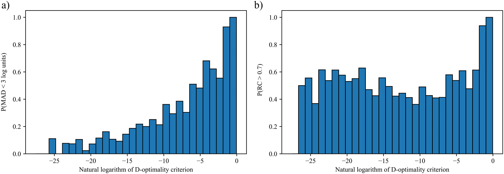 | ||
| Fig. 2 Probability distributions of obtaining LFERs with a) MAD < 3log units for the Menshutkin reaction and b) RC > 0.7 for the Menshutkin reaction. | ||
3.2 Analysis of selection spaces
Next, we conduct a thorough analysis to characterise and compare the four selection spaces defined in section 2.2. For each selection space, the number of solvents, the standard deviation and mean of each solvent property, and the average standard deviation over all these solvent properties are summarised in Table 1. It should be noted that ϕ and ψ are not considered in the analysis as they are primarily indicative of the structural characteristics of solvents rather than their broader physicochemical properties. The number of solvents in each selection space increases in going from strictly real solvents with experimental properties (SS1) to physically constrained molecules with model-predicted properties (SS2), onto chemically constrained molecules with model-predicted properties (SS3) and finally to structure-free “molecules” defined by continuous property values (SS4). The standard deviation and mean are used to characterise the similarities between the selection spaces. For SS4, the standard deviations are set to be the standard deviation of a uniform distribution based on the given bounds for each property. As can be expected, SS4 exhibits the largest standard deviations for all the properties due to the extensive property ranges. Notably, although SS1 contains the fewest solvents, it exhibits larger standard deviations for n2 and ε than SS2 and SS3, which indicates there is less homogeneity in SS1 in terms of these two properties. By contrast, although they contain more solvents, the diversity of SS2 and SS3 is constrained by the available atom groups that can be combined to define the solvent molecules. As a result, many of the solvents in SS2 and SS3 belong to the same chemical families and do not contribute to solvent diversity of these selection spaces. This is also exemplified by the larger standard deviation of n2 and ε for SS2 than those for SS3, as a result of the incorporation of the four single-molecule groups in SS2 that are not present in SS3. The other 322 solvents in SS2 are assembled from multiple atom groups and also belong to SS3. Thus, they do not account for the superior diversity of SS2 in terms of n2 and ε, and the four single-molecule groups greatly contribute to the solvent diversity in SS2. The overall diversity of the four selection spaces can be ranked based on the average standard deviations as: SS2 < SS3 < SS1 < SS4. It should also be noted that the mean values of each property in SS3 and SS4 are generally larger than those in SS1 and SS2, probably due to the presence of a large number of unphysical solvents.| Number of solvents | SS1 | SS2 | SS3 | SS4 | ||||
|---|---|---|---|---|---|---|---|---|
| 178 | 326 | 4398 | Infinite | |||||
| Mean | STD | Mean | STD | Mean | STD | Mean | STD | |
| A | 0.090 | 0.174 | 0.113 | 0.153 | 0.332 | 0.280 | 0.500 | 0.289 |
| B | 0.308 | 0.236 | 0.408 | 0.174 | 0.507 | 0.286 | 0.750 | 0.433 |
| n 2 | 2.096 | 0.202 | 2.307 | 0.094 | 2.351 | 0.079 | 2.500 | 0.866 |
| γ | 0.410 | 0.108 | 0.394 | 0.110 | 0.525 | 0.161 | 0.500 | 0.289 |
| ε | 0.112 | 0.178 | 0.121 | 0.109 | 0.096 | 0.070 | 1.005 | 0.574 |
| Average | 0.180 | 0.128 | 0.175 | 0.490 | ||||
We further analyse the property distributions in the four selection spaces using box plots in Fig. 3. The box plot for each solvent property in SS4 is approximated using a set of evenly distributed values between the associated upper and lower bounds. With all the outliers taken into consideration, the ranges of properties covered by SS1 are generally larger (n2 and ε) than or comparable (A, B and γ) to those covered by SS2 and SS3. SS2 shows the smallest coverage for all the properties except ε as single-molecule group N-methylformamide possesses an extreme dielectric constant of 1.816 after scaling. Similarly to the mean values, the median values of most solvent properties are larger in SS3 and SS4 compared to those in SS1 and SS2 due to the presence of many unphysical solvents. Notably, SS1 and SS2, which consist only of physically constrained solvents, show strong negative skewness for properties A and ε, a feature that is not seen in SS3 and SS4.
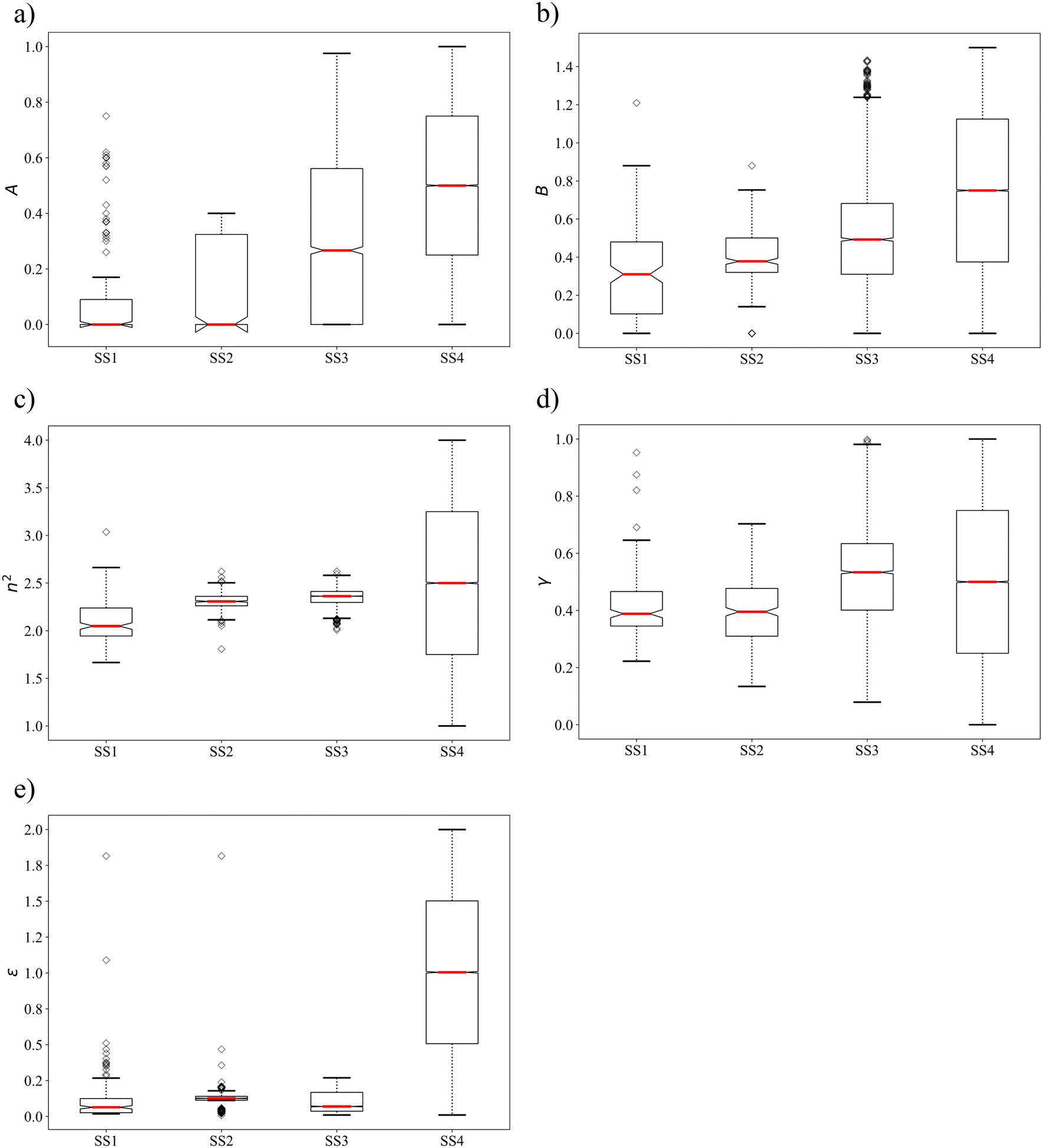 | ||
| Fig. 3 Box plots of the distributions of solvent property values in the four selection spaces a) A, b) B, c) n2, d) γ and e) ε. | ||
To better visualise the (dis)similarities between different selection spaces, the t-distributed stochastic neighbor embedding (t-SNE) algorithm69 is adopted as a dimension–reduction approach that preserves similarity information from high-dimensional data points in the reduced-dimensional space. The results are shown in Fig. 4, with all data points colour-coded based on lnkL,QM values except those in SS3 as QM calculations are not available for all the solvents in this selection space due to the overwhelmingly large number of calculations required. SS4 is not shown as it is inherently homogeneous. In the t-SNE visualisation, data points are found to form clusters according to interpoint similarities. We find that clusters generally form in accordance with chemical families, i.e., solvents that share one (or more) common functional group(s) or structural feature(s) belong to the same cluster. SS3 forms the most clusters of various sizes and thus displays the most coverage of the low-dimensional space. SS2 forms the fewest clusters, and there is a large SS2 cluster overlapping with one of the SS3 clusters due to the fact SS2 and SS3 share 322 common solvents. Compared to SS2, solvents in SS1 form smaller but more numerous clusters that scatter sparsely in the low-dimensional space. Additionally, the solvents in SS1 also lead to a larger range of lnkL,QM values than those in SS2.
 | ||
| Fig. 4 The two-dimensional t-SNE visualisation of solvent properties in SS1 (triangles), SS2 (squares) and SS3 (circles). The color scale indicated the lnkL,QM values for the corresponding solvents, where available. | ||
All the results in this section consistently indicate that the diversity ranking of the selection spaces is as follows: SS4 > SS1 ≈ SS3 > SS2, a finding that is consistent with the standard deviation analysis.
3.3 Design of optimal computer experiments
The D-optimality criterion is applied to identify an optimal set of computer experiments, i.e., a set of training solvents, from each selection space. D-optimal designs are generated using Fedorov's algorithm for SS1, SS2 and SS3 and using the NLP optimisation approach for SS4. A D-optimal set of 9 solvents is generated for each selection space. It should be noted that 9 is the minimum number of solvents required to perform MLR for eqn (1). The D-optimality criterion values of the D-optimal solvent sets identified from SS1, SS2, SS3 and SS4 are 9.63 × 10⁻¹, 8.86 × 10⁻³, 1.91 × 10⁻³ and 1.64 × 10⁵, respectively. The identities of the D-optimal solvents generated from each selection space are shown in Table 2 except SS4 as no corresponding chemical structures are associated with these hypothetical solvents. The MBDoE sets from SS1, SS2 and SS3 meet minimum expectations of chemical diversity in that, in each set, no two molecules belong to the same chemical class, i.e., have exactly the same set of functional groups.| Solvent | SS1 | SS2 | SS3 |
|---|---|---|---|
| a Indicates other constitutional isomers exist. | |||
| 1 | N-Methylformamide | Nitromethanol | Nitromethanol |
| 2 | m-Cresol | DMSO | 1,2,3,4-Tetraamino-5-fluoro-6-methoxybenzenea |
| 3 | Tetrahydrothiophene-S,S-dioxide | Acetonitrile | Acetic acid(GC) |
| 4 | Carbon tetrachloride | Benzene(GC) | Diiodomethane(GC) |
| 5 | n-Pentane | 2,3,4-Trimethyl-but-2-ene-1-ol | 1,2,3-Triamino-4,5-dichloro-6-nitromethylbenzenea |
| 6 | Tributylphosphate | 1-Ethoxy-2-methyl-prop-1-enea | Tetramethylethylene |
| 7 | Formic acid | Chloroform | Benzene(GC) |
| 8 | Diiodomethane | 2-Methylhexane | 1,5-Diamino-3,4,4-trimethyl-pent-2-enea |
| 9 | Benzene | N-Methylformamide | Dichloromethanol |
Radar charts are employed to illustrate the relationship between the MBDoE solvents and the other candidate solvents in each selection space (Fig. 5). In these radar charts, each solvent descriptor/property is represented by a radial axis normalised with the maximum value for that descriptor among all candidate solvents within the same selection space. Each solvent is represented by a polygon that intersects each property axis at the point corresponding to the solvent's normalised property value. The candidate solvents in each selection space are represented by red polygons, and the MBDoE solvents are represented by blue polygons. The red areas on the radar plots reflect the number of solvents available in each selection space, as well as the distributions of the property values. The radar chart for SS4 is distinguished by a red background since this selection space is formed by hypothetical solvents defined by all combinations of the continuous property values. Generally, the property values of the MBDoE solvents, illustrated by blue lines, encompass the entire range of property values. These MBDoE solvents typically exhibit either minima or maxima across all descriptors to achieve maximum chemical diversity within the respective selection space. It can however be seen in SS1, SS2 and SS3 that some of the properties take on intermediate values. This is due to the finiteness of the set of allowed combinations of the property values, which is limited to the number of solvents in the selection space. The MBDoE formulation makes it possible to generate a maximally informative set of training solvents by projecting the discrete space onto the constrained space of continuous solvent properties.
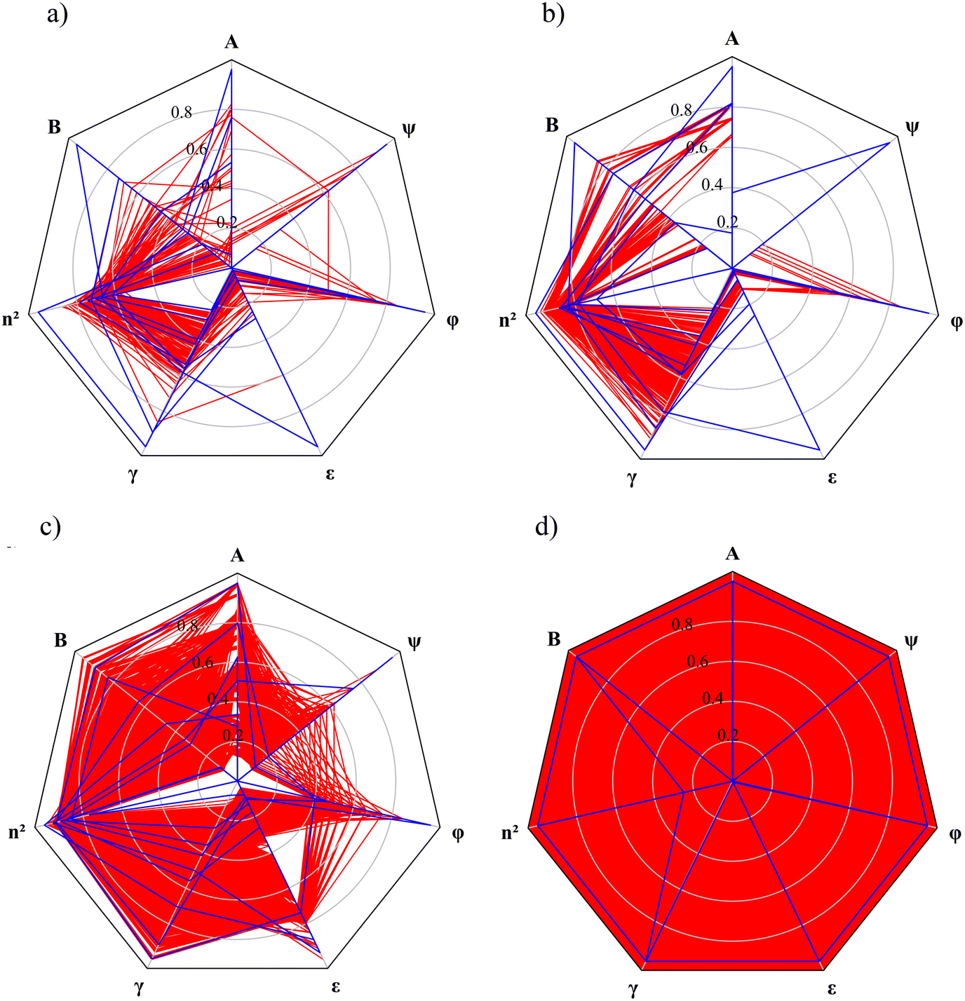 | ||
| Fig. 5 Radar charts of the descriptors of the MBDoE solvents (blue) generated from a) selection space 1, b) selection space 2, c) selection space 3 and d) selection space 4. Candidate solvents are denoted by red lines. | ||
When comparing the radar plots, it is important to consider that the ranges of the unscaled property values are different across the selection spaces, a factor that may affect the performance of the resulting solvatochromic equations. The spans of the unscaled property values are visualised using a parallel coordinates plot in Fig. 6. SS4 leads to extreme MBDoE solvents in terms of property values as well as the widest range of lnkL,QM values, although it does not cover solvents in the mid-range of lnkL,QM values as the other three selection spaces do. All the other MBDoE sets also give reasonably wide ranges of lnkL,QM, in spite of the narrower ranges of n2 and ε values. However, MBDoE solvents with extremely low lnkL,QM values are only identified from SS4. It can also be seen that in general larger dielectric constants lead to larger lnkL,QM, except in the region where lnkL,QM becomes exceedingly large. In terms of the ranges of the property values for SS1, SS2 and SS3, the D-optimal set for SS1 affords the largest variation in n2 and ε while the D-optimal set for SS3 prevails in the other solvent properties with SS1 only slightly narrower.
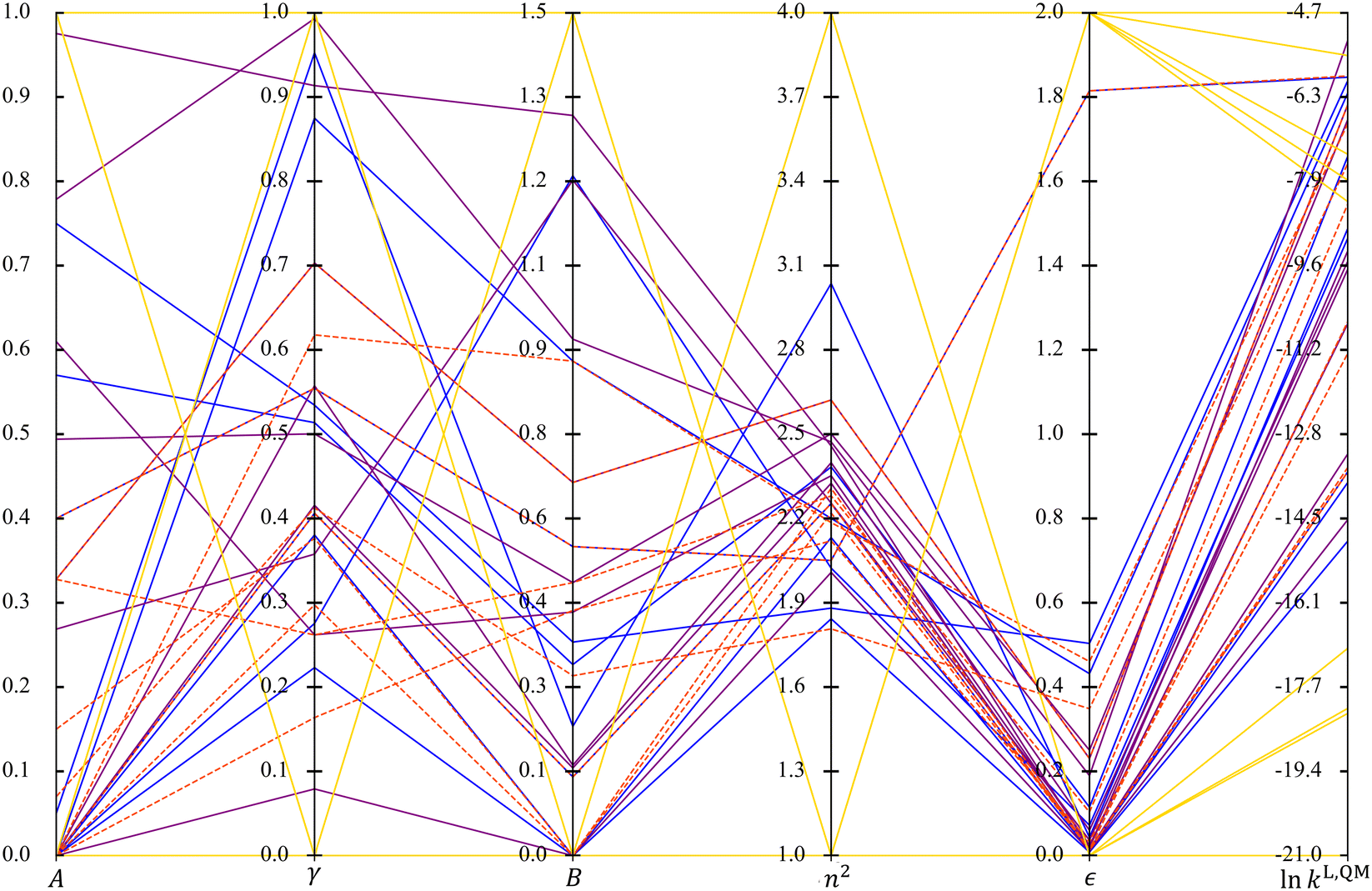 | ||
| Fig. 6 Parallel coordinates plot of solvent properties (A, γ, B, n2, ε) and lnkL,QM across the four sets of MBDoE solvents: SS1 (solid blue), SS2 (dashed red, dashed lines are used here to distinguish overlapped lines), SS3 (solid purple) and SS4 (solid yellow). | ||
In summary, all MBDoE solvent sets show chemical diversity in the functional groups/structural features they contain and in their property values, where they encompass the entire range of values in the corresponding selection spaces even when selecting as few as 9 solvents. Comparison across the training sets shows that the D-optimal set for SS4 exhibits the largest range of property values, followed by SS1, SS3 and then SS2. The property values of the candidate solvents and the D-optimal solvents of SS1, SS2 and SS3 and the property values of the D-optimal solvents of SS4 are given in the Zenodo online repository as ESI.†
3.4 Performance of the regressed surrogate models
In section 3.1, it was shown that when the D-optimality criterion value is maximised, there is a very high chance (near 100%) of obtaining a LFER with good performance, i.e., a MAD < 3log units and a RC > 0.7. We thus proceed to regress the LFERs using the D-optimal solvent sets identified in section 3.3 and verify their performance. To generate the training data for the regression of the LFER coefficients, eqn (1), the rate constants of the Menshutkin reaction (Fig. 7) are calculated by following the QM method described in section 2.4 for the solvents in the D-optimal set identified in each selection space. All the regressed model coefficients can be found in section S1 in the ESI† as well as in the Excel sheet provided in the Zenodo online repository. The resulting models are evaluated against the test set (SS2) by calculating the corresponding MAD and RC.
 | ||
| Fig. 7 The Menshutkin reaction between pyridine and phenacyl bromide. | ||
The results are visualised using the parity plots in Fig. 8 where the rate constants predicted by the regressed LFERs, lnkL,LFER, are compared to the QM rate constants, lnkL,QM. As can be seen, most of the LFERs show good performance in both MAD and RC. The selection space that results in the smallest testing MAD (1.304log units) is SS3, followed by SS2 (1.540log units) and then SS1 (2.136log units). They are all smaller than 3log units. However, SS4, which contains hypothetical solvents, leads to the largest testing MAD of 9.339log units due to the significant systematic deviations observed for nearly all the solvents in the test set. Systematic deviations of a similar nature can also be observed for the clusters located around the mid-range of QM rate constants in the parity plots of the other selection spaces. This may be understood by realising that when applying the D-optimality criterion to a linear model, such as eqn (1), those solvents exhibiting extremely high or extremely low property values tend to be selected, as indicated in Fig. 5. Consequently, the coverage of the mid-range solvents is not sufficiently dense, leading to these solvents falling outside the validity domain of the regressed equation70 and a corresponding deterioration in the predictive performance of the surrogate models for solvents with moderate property values. This issue of validity domain is severe especially when the assumption of a linear relationship is not reflective of reality and when the shape of the test set is irregular.
 | ||
| Fig. 8 Parity plots of lnkL,LFERvs. lnkL,QM of the Menshutkin reaction for the solvatochromic equations generated from a) SS1, c) SS2, e) SS3 and g) SS4 and parity plots of the lnkL,LFER solvent rankings vs. the lnkL,QM solvent rankings for the Menshutkin reaction for the solvatochromic equations generated from b) SS1, d) SS2, f) SS3 and h) SS4. The insets show a close-up of the parity plots for the top 20 solvent rankings. | ||
To further understand the nature of the systematic deviations, additional D-optimal solvent sets with 13 and 49 solvent are obtained for SS2 and used to derive two further LFERs. The relationship between the training and testing solvents within SS2 is visualised using the t-SNE method, with colour-coding denoting the absolute deviation between the QM model and the LFER model (Fig. 9). The MBDoE solvents used for training are highlighted with red circles. SS2 is chosen because using the same selection space and test set facilitates tracking the relationship between the training data points and the data points that exhibit systematic deviations. It is clearly seen in Fig. 9a that the solvents that exhibit large deviations fall mostly into one cluster (shown by a red rectangle) which is not sampled, given only 9 training solvents are used. In other words, the cluster is outside the validity domain of the regressed surrogate model. When we increase p (i.e., the number of MBDoE solvents) to 13 (Fig. 9b), one data point is included in the previously low accuracy cluster and a significant improvement is seen for all the solvents in this cluster. When p is further increased to 49 (Fig. 9c), and more data points are sampled in the cluster, the absolute deviations for all the data points in the cluster become very small, indicating that the mid-range solvents are adequately sampled and the validity domain now includes the corresponding region. These results are indicative of the overall nonlinear nature of the QM model. Increasing the size of the training dataset to improve the sampling coverage offers a strategy to mitigate the systematic deviations, without increasing model complexity.
 | ||
| Fig. 9 The t-SNE visualisation of the solvents in SS2 for varying number of MBDoE solvents a) p = 9; b) p = 13; and c) p = 49. The absolute deviations between the QM and the LFER models are shown on the colour scale and the MBDoE solvents are denoted by red circles. The red rectangle highlights the solvents that exhibit the largest deviation for the 9-solvent training set. | ||
Next, we evaluate the predictive performance of the LFER for the solvent rankings in order of the reaction rate constants, as seen in the parity plots of RQMvs. RLFER shown in Fig. 8e–h. It can be seen that all the LFERs yield RCs greater than 0.8 with the RCs corresponding to SS1, SS3 and SS4 greater than 0.9. Notably, the LFER corresponding to SS4 provides the best RC value (0.984), though the testing MAD is the worst among all the models evaluated. This reinforces the assumption that a linear model, albeit inadequate to capture the sophisticated mathematical formalism of the QM model, can capture general trends based on the use of data at the extremes of the selection space. The LFER corresponding to SS2 provides the worst RC (0.803) among the four LFERs, when 9 solvents are used in the training set. This relatively poorer performance may seem to conflict with the fact that SS2 is also the test set. However, this LFER offers reasonable performance in that it provides both smaller MAD and larger RC than the threshold values used in section 3.1. The insets in Fig. 8e–h show the parity plots of the top 20 solvents in terms of lnkL,QM values, and consistent performance can be seen with the RC values calculated for all the solvents in the test set. The regression coefficients in these LFER models (see section S1 in the ESI†) indicate that solvents with high hydrogen bond acidity, hydrogen bond basicity, and surface tension consistently lead to increased rate constants, and thus, higher solvent rankings. Such a favourable solvent effect is to be expected for solvents that can form hydrogen bonds (as donor or acceptor), as such solvents can significantly stabilise the transition state of the Menshutkin reaction, where charge separation occurs, relative to the neutral reactants.71
To summarise the key findings in this section, in general, the prediction of reaction rate constants can be achieved within a 20-fold difference from the QM prediction using only a minimum number of training solvents, with the exception of SS4. However, with a small number of solvents, systematic deviations are consistently observed for mid-range lnkL,QM solvents due to the violation of the validity domain of the resulting model. Satisfactory prediction of solvent rankings in order of reaction rate constants can be achieved by almost all the solvatochromic equations regressed from the D-optimal solvent sets except SS2.
3.5 Factors that affect the performance of the surrogate model
Notwithstanding the promising results that have been obtained in the previous sections, the use of a minimal number of training solvents and the linear structure of the surrogate model may limit model performance. In this section, we explore the impact of increasing p in the D-optimal set, of incorporating quadratic terms into the LFER (eqn (2)) and of maintaining the similarity of the selection space to the test set. The interplay of these factors is also taken into consideration. Since the sizes of SS3 and SS4 are very large such that the computational time required to identify larger D-optimal sets becomes unmanageable, only SS1 and SS2 are chosen for the investigation. With newly added quadratic terms in the QFER (eqn (2)), the minimum number of training data points required becomes p = 13. The relationship between the model performance and p for two selection spaces (SS1 and SS2) and two surrogate models (linear and quadratic) is shown in Fig. 10 using the natural logarithms of D-optimality criterion values, MAD, RC and RMSDR-20 as performance indicators.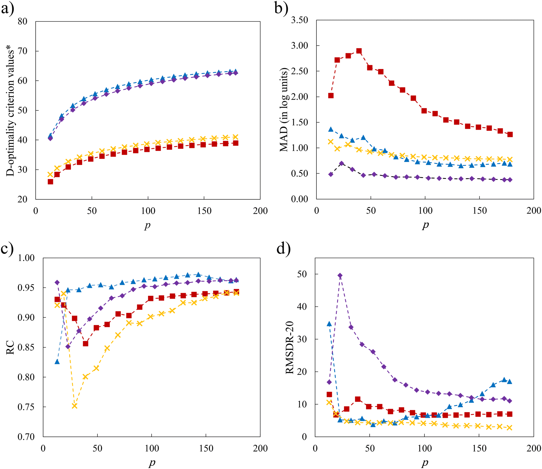 | ||
| Fig. 10 Natural logarithm of D-optimality criterion value and performance metric as a function of p for the LFER using SS1 (SS1-L, red squares), the QFER using SS1 (SS1-Q, blue triangles), the LFER using SS2 (SS2-L, yellow crosses) and the QFER using SS2 (SS2-Q, purple diamonds): a) natural logarithms of D-optimality criterion values (*here D-optimality criterion values are computed, in a different way, based on mean-centered and unit-variance properties since this enables the identification of solvents with mid-range property values when using the quadratic model) b) MAD, c) RC and d) RMSDR-20. The first data point in each graph corresponds to a training set of 9 solvents for the linear models and 13 solvents for the quadratic models. | ||
As shown in Fig. 10, the linear model associated with SS1 (SS1-L) shows the worst performance with the smallest D-optimality criterion values across all values of the number of solvents in the training set that are considered. The MAD for SS1-L initially increases until it reaches a peak at p = 39 solvents, after which it subsequently decreases. This behaviour can be explained by our conjecture that the initial training sets lack a sufficient number of mid-range solvents with moderate property values, leading to the overall poor performance of the model. As the number of solvents increases, the validity domain of the model is expanded to cover these solvents. Performance is also addressed by introducing quadratic terms, as a quadratic model may better describe the underlying QM model. With these quadratic terms, a significant enhancement of model performance is seen over the entire range of values of p for D-optimality criterion values, MAD and RC. For RMSDR-20, performance is less consistent with SS1-Q exhibiting worse performance when many solvents (p > 100) are used for training.
Next, we consider the scenario where the selection space is identical to the test set, i.e., SS2 is employed to generate the D-optimal solvent sets, for the purpose of further investigating the importance of the similarity between the selection space and the test set as this may have an impact on the validity domain of the resulting model. As seen in Fig. 10a, the linear model of selection SS2 (SS2-L) shows slightly larger D-optimality criterion values compared to SS1-L over the entire range of p but much smaller compared to the quadratic models. Below p = 59 solvents, SS2-L generates smaller MADs than both SS1-L and SS1-Q. When p further increases, the MAD varies only slightly and becomes slightly larger than that for SS1-Q. Overall, both the incorporation of quadratic terms and the utilisation of similar training data to the testing data benefit the performance of the surrogate model and the impact of similarity appears to be most important when p is small.
Despite the general improvement in the MAD at small p values, systematic deviations for the mid-range solvents are still observed for all the surrogate models that have been discussed so far. The cooperative impact of quadratic terms and the similarity between the selection space and the test set are then investigated (Fig. 10b). SS2-Q yields smaller MADs than those in the other three scenarios over the entire range of p values. Even with the minimal number p of 13 solvents, a testing MAD of 0.481log unit is achieved and the systematic deviations for the mid-range solvents can be largely eliminated, as shown in Fig. 11. These results indicate that the MBDoE approach holds promise for generating a minimal number of solvents with a comparable amount of information content to a much larger solvent set, when the regression model adequately describes the QM function and the solvent selection space is similar to the test set.
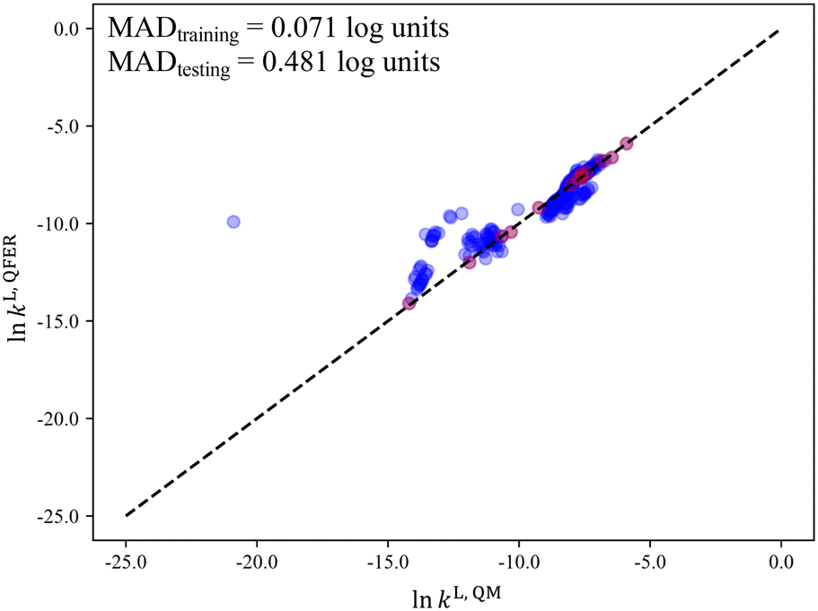 | ||
| Fig. 11 The parity plot of lnkL,QFERvs. lnkL,QM of the Menshutkin reaction for the quadratic free energy relationship generated from SS2 (red: training data, blue: testing data). The outlier corresponds to 2-ethyl-6-methylaniline (or its other positional isomers) with a lnkL,QM of −20.89. Its extremely low rate constant results from an abnormally small dielectric constant (0.8), predicted by the group contribution method.26 Dielectric constants are typically defined as being greater than 1 for non-vacuum medium, demonstrating a rare failure of the group contribution method used in this instance. | ||
Next, the relationship between RC and the number of training solvents is investigated (Fig. 10c). Despite inconsistent trends when p is small, all models level off between RC = 0.90 and RC = 0.95. The RC of model SS1-Q starts to plateau quickly, at only p = 23 solvents. Overall, SS1-Q gives the best ranking prediction performance across the range of p values, followed by the SS2-Q, SS1-L and then SS2-L. Quadratic models are therefore found to be better than linear models at capturing the overall trend of the rankings. The better overall RC performance from SS1 may be due to the positive impact brought by the greater diversity in the selection space/training set.
We further investigate the ability of the models to correctly identify and rank the solvents with large rate constants using RMSDR-20 as the metric (Fig. 10d). Since RMSDR-20 quantifies the differences between the rankings predicted by the QM model and the surrogate models for the top 20 solvents, an RMSDR-20 below 10 would most likely ensure the surrogate models also predict these solvents to have high rankings. Both linear models show more consistent performance as a function of p compared to the quadratic models, with SS2-L performing slightly better overall. SS1-Q exhibits a low RMSDR-20 for p values between 23 and 113 solvents, but this increases for p > 113. SS2-Q begins with a low RMSDR-20 and peaks at nearly 50 for p = 23 solvents, after which it decreases until it reaches around 10.
To summarise, depending on the performance metric under evaluation, different design schemes are needed to design optimal computer experiments with optimal model performance. SS2-Q is the best for achieving a small MAD regardless of the number of training solvents. All models require a relatively large p to achieve a high RC, with SS1-L providing good performance at p > 23. However, SS1-L, SS2-L and SS2-Q all have acceptable RC values at low p values. SS1-Q and SS2-L are very effective at producing a correct ranking of high rate constant solvents with a small p.
4 Conclusions
In this work, we have demonstrated the effectiveness of using the D-optimality criterion to the selection of a small set of training data (solvents). This approach has been found to lead to an increased likelihood of obtaining simple surrogate models with good predictive performance in terms of reaction rate constant values and the associated solvent rankings. In our current work, LFERs have been regressed to the outputs of deterministic computer experiments, i.e., QM calculations of liquid-phase reaction rate constants. We have generated four D-optimal solvent sets of 9 solvents from four selection spaces with varying characteristics. The LFERs regressed from these MBDoE solvent set generally yield satisfactory MADs, with the set of hypothetical solvents being the exception due to an inadequate validity domain. Remarkably, the LFERs obtained from such small data sets achieve exceptional performance in predicting solvent rankings, providing a valuable tool for comparing reaction kinetics in different solvents.We have also highlighted several considerations for researchers who would like to design computer experiments using a similar approach. First, the inclusion of quadratic terms in the surrogate model results in a marked improvement in the quantitative accuracy of predictions for a given number of training solvents. Second, if accurate quantitative prediction is targeted, the selection space for the training data should be similar to the test set, i.e., one should design computer experiments in alignment with the intended application domain. Finally, the diversity of the selection space appears to play an important role in the reliability of qualitative (ranking) predictions.
Our findings have shown the potential usefulness of traditional MBDoE techniques for the identification of effective computer experiments that make it possible to capture complex relationships between molecular structure and physicochemical properties with remarkably few data points. The applicability of this approach should be tested on other free energy-dependent properties. The findings, along with our previous work,56 have also shown that it is beneficial to integrate MBDoE into the framework of computer-aided molecular design, since the MBDoE technique can reduce the number of solvents required to train a satisfactory surrogate model for property prediction, thereby can reducing the resources and time needed to design new molecules. The DoE-QM-CAMD method we have developed56 is one of many potential applications that can benefit from this approach. It has been found to facilitate the design of solvents that optimise reaction kinetics in chemical and pharmaceutical synthesis.
Note
The chemical feasibility of the solvents in SS2 and SS3 refers to the fulfilment of expected atom valencies when assembling pre-defined atom groups into molecules. Further evaluation is required to ensure the chemical stability of selected solvents.Data availability
Data underlying this article and not available in the references cited are available in the ESI† and on the Zenodo repository (https://doi.org/10.5281/zenodo.8396100) under a CC BY license. A list of the files/directories in the Zenodo repository and the information contained therein are provided in section S2 of the ESI.†Author contributions
Lingfeng Gui: conceptualization, methodology, software, testing, investigation, data curation, writing – original draft, visualization. Alan Armstrong: conceptualization, methodology, writing – review & editing, supervision, funding acquisition. Amparo Galindo: conceptualization, methodology, testing, writing – review & editing, supervision, funding acquisition. Fareed Bhasha Sayyed: conceptualization, writing – review & editing, supervision. Stanley P. Kolis: conceptualization, writing – review & editing, supervision. Claire S. Adjiman: conceptualization, methodology, testing, writing – review & editing, supervision, project administration, funding acquisition.Conflicts of interest
There are no conflicts to declare.Acknowledgements
Funding from Eli Lilly and Company and the UK EPSRC, through the PharmaSEL-Prosperity Programme (EP/T005556/1), is gratefully acknowledged. AG acknowledges the funding of a Research Chair by the Royal Academy of Engineering and Eli Lilly and Company (RCSRF1819/7/33). The Imperial College Research Computing Service (DOI: https://doi.org/10.14469/hpc/2232) is also gratefully acknowledged for providing support and resources for the quantum mechanical calculations.Notes and references
- C. Reichardt and T. Welton, in Solvent Effects on the Rates of Homogeneous Chemical Reactions, John Wiley & Sons, Ltd, 2010, ch. 5, pp. 165–357 Search PubMed.
- L. Shuai and J. Luterbacher, ChemSusChem, 2016, 9, 133–155 CrossRef PubMed.
- M. A. Mellmer, C. Sanpitakseree, B. Demir, P. Bai, K. Ma, M. Neurock and J. A. Dumesic, Nat. Catal., 2018, 1, 199–207 CrossRef CAS.
- J. C. Schleicher and A. M. Scurto, Green Chem., 2009, 11, 694–703 RSC.
- M. Erny, M. Lundqvist, J. H. Rasmussen, O. Ludemann-Hombourger, F. Bihel and J. Pawlas, Org. Process Res. Dev., 2020, 24, 1341–1349 CrossRef CAS.
- K. Liang, T. R. Rooney and R. A. Hutchinson, Ind. Eng. Chem. Res., 2014, 53, 7296–7304 CrossRef CAS.
- X. Li and A. L. Dunn, Org. Process Res. Dev., 2022, 26, 795–803 CrossRef.
- J. Ho and M. Z. Ertem, J. Phys. Chem. B, 2016, 120, 1319–1329 CrossRef.
- Y. Chung and W. H. Green, J. Phys. Chem. A, 2023, 127, 5637–5651 CrossRef.
- M. Taylor, H. Yu and J. Ho, J. Phys. Chem. B, 2022, 126, 9047–9058 CrossRef.
- S. Park, H. Han, H. Kim and S. Choi, Chem. – Asian J., 2022, 17, e202200203 CrossRef PubMed.
- Y. Chung and W. H. Green, Chem. Sci., 2024, 15, 2410–2424 RSC.
- D. M. Hawkins, J. Chem. Inf. Comput. Sci., 2004, 44, 1–12 CrossRef.
- R. W. Taft, M. H. Abraham, R. M. Doherty and M. J. Kamlet, J. Am. Chem. Soc., 1985, 107, 3105–3110 CrossRef.
- S. C. Rutan, P. W. Carr and R. W. Taft, J. Phys. Chem., 1989, 93, 4292–4297 CrossRef.
- A. Pagliara, G. Caron, G. Lisa, W. Fan, P. Gaillard, P.-A. Carrupt, B. Testa and M. H. Abraham, J. Chem. Soc., Perkin Trans. 2, 1997, 2639–2644 RSC.
- M. H. Abraham, H. S. Chadha, G. S. Whiting and R. C. Mitchell, J. Pharm. Sci., 1994, 83, 1085–1100 CrossRef.
- J. Barbosa, G. Fonrodona, I. Marqués, V. Sanz-Nebot and I. Toro, Anal. Chim. Acta, 1997, 351, 397–405 CrossRef.
- E. Casassas, G. Fonrodona and A. de Juan, J. Solution Chem., 1992, 21, 147–162 CrossRef.
- J. M. Harris, M. R. Sedaghat-Herati, S. P. McManus and M. H. Abraham, J. Phys. Org. Chem., 1988, 1, 359–362 CrossRef.
- M. Folić, C. S. Adjiman and E. N. Pistikopoulos, AIChE J., 2007, 53, 1240–1256 CrossRef.
- H. Struebing, Z. Ganase, P. G. Karamertzanis, E. Siougkrou, P. Haycock, P. M. Piccione, A. Armstrong, A. Galindo and C. S. Adjiman, Nat. Chem., 2013, 5, 952–957 CrossRef PubMed.
- M. J. Kamlet, J. L. M. Abboud, M. H. Abraham and R. W. Taft, J. Org. Chem., 1983, 48, 2877–2887 CrossRef.
- M. H. Abraham, Chem. Soc. Rev., 1993, 22, 73–83 RSC.
- A. F. Lagalante, M. Spadi and T. J. Bruno, J. Chem. Eng. Data, 2000, 45, 382–385 CrossRef.
- T. Sheldon, C. Adjiman and J. Cordiner, Fluid Phase Equilib., 2005, 231, 27–37 CrossRef.
- A. Duereh, A. Anantpinijwatna and P. Latcharote, Appl. Sci., 2020, 10, 8480 CrossRef.
- B. Williams and S. Cremaschi, Chem. Eng. Res. Des., 2021, 170, 76–89 CrossRef.
- G. Franceschini and S. Macchietto, Chem. Eng. Sci., 2008, 63, 4846–4872 CrossRef.
- A. C. Atkinson, A. N. Donev and R. D. Tobias, Optimum experimental designs, with SAS, Oxford University Press, Oxford, 2007 Search PubMed.
- S. Asprey and S. Macchietto, J. Process Control, 2002, 12, 545–556 CrossRef.
- B. Jones, K. Allen-Moyer and P. Goos, J. Qual. Technol., 2021, 53, 369–382 CrossRef.
- B. Smucker, M. Krzywinski and N. Altman, Nat. Methods, 2018, 15, 559–560 CrossRef.
- D. S. Wicaksono, A. Mhamdi and W. Marquardt, Chem. Eng. Sci., 2014, 115, 167–176 CrossRef.
- A. Tsichla, C. Severins, M. Gottfried and W. Marquardt, Ind. Eng. Chem. Res., 2019, 58, 13517–13532 CrossRef CAS.
- T. O. Oliyide, M.Sc. Thesis, Imperial College London, 2014 Search PubMed.
- S. H. Kim and F. Boukouvala, Comput. Chem. Eng., 2020, 140, 106847 CrossRef CAS.
- A. Svalova, P. Helm, D. Prangle, M. Rouainia, S. Glendinning and D. J. Wilkinson, Data-Centric Eng., 2021, 2, e12 CrossRef.
- S. S. Garud, I. A. Karimi and M. Kraft, Comput. Chem. Eng., 2017, 106, 71–95 CrossRef CAS.
- V. R. Joseph, Qual. Eng., 2016, 28, 28–35 CrossRef.
- L. Xing, H. Jiang, S. Wang, V. J. Pinfield and J. Xuan, Chem. Eng. J., 2023, 454, 139997 CrossRef CAS.
- B. W. Lee, J. J. Peterson, K. Yin, G. S. Stockdale, Y. C. Liu and A. O'Brien, Chem. Eng. Res. Des., 2020, 156, 495–506 CrossRef.
- J. Duchon, Constructive Theory of Functions of Several Variables, Berlin, Heidelberg, 1977, pp. 85–100 Search PubMed.
- S. S. Miriyala, P. Mittal, S. Majumdar and K. Mitra, Chem. Eng. Sci., 2016, 140, 44–61 CrossRef.
- M. Bracconi and M. Maestri, Chem. Eng. J., 2020, 400, 125469 CrossRef.
- J. Eason and S. Cremaschi, Comput. Chem. Eng., 2014, 68, 220–232 CrossRef.
- T. Zhou, Z. Qi and K. Sundmacher, Chem. Eng. Sci., 2014, 115, 177–185 CrossRef.
- A. Klamt, F. Eckert and W. Arlt, Annu. Rev. Chem. Biomol. Eng., 2010, 1, 101–122 CrossRef CAS PubMed.
- L. Kaufman and P. J. Rousseeuw, Finding groups in data: an introduction to cluster analysis, John Wiley & Sons, 2009 Search PubMed.
- S. Wan, R. C. Sinclair and P. V. Coveney, Philos. Trans. R. Soc., A, 2021, 379, 20200082 CrossRef CAS PubMed.
- T. W. Simpson, J. Peplinski, P. N. Koch and J. K. Allen, On the Use of Statistics in Design and the Implications for Deterministic Computer Experiments, in 9th International Design Theory and Methodology Conference, 1997, vol. 3 Search PubMed.
- L. Gui, A. Armstrong, A. Galindo, F. B. Sayyed, S. P. Kolis and C. S. Adjiman, 32nd European Symposium on Computer Aided Process Engineering, Elsevier, 2022, vol. 51, pp. 607–612 Search PubMed.
- P. Winget, D. M. Dolney, D. J. Giesen, C. J. Cramer and D. G. Truhlar, Minnesota Solvent Descriptor Database, 2021, https://comp.chem.umn.edu/solvation/mnsddb.pdf Search PubMed.
- A. V. Marenich, C. J. Cramer and D. G. Truhlar, J. Phys. Chem. B, 2009, 113, 6378–6396 CrossRef CAS.
- E. Grant, Y. Pan, J. Richardson, J. R. Martinelli, A. Armstrong, A. Galindo and C. S. Adjiman, 13th International Symposium on Process Systems Engineering (PSE 2018), Elsevier, 2018, vol. 44, pp. 2437–2442 Search PubMed.
- L. Gui, Y. Yu, T. O. Oliyide, E. Siougkrou, A. Armstrong, A. Galindo, F. B. Sayyed, S. P. Kolis and C. S. Adjiman, Comput. Chem. Eng., 2023, 177, 108345 CrossRef CAS.
- P. de Aguiar, B. Bourguignon, M. Khots, D. Massart and R. Phan-Than-Luu, Chemom. Intell. Lab. Syst., 1995, 30, 199–210 CrossRef.
- G. R. Kocis and I. E. Grossmann, Comput. Chem. Eng., 1989, 13, 307–315 CrossRef CAS.
- A. Drud, SBB: A New Solver for Mixed Integer Nonlinear Programming, 2001 Search PubMed.
- Q. Chen, R. Paulavičius, C. S. Adjiman and S. García-Muñoz, AIChE J., 2018, 64, 3944–3957 CrossRef CAS.
- D. S. Watkins, Fundamentals of matrix computations, Wiley, New York, 1991, p. 84 Search PubMed.
- H. Eyring, J. Chem. Phys., 1935, 3, 107–115 CrossRef CAS.
- K. J. Laidler and M. C. King, J. Phys. Chem., 1983, 87, 2657–2664 CrossRef CAS.
- E. Wigner, J. Chem. Phys., 1937, 5, 720–725 CrossRef.
- Y. Zhao and D. G. Truhlar, Theor. Chem. Acc., 2008, 120, 215–241 Search PubMed.
- L. A. Curtiss, P. C. Redfern, K. Raghavachari, V. Rassolov and J. A. Pople, J. Chem. Phys., 1999, 110, 4703–4709 CrossRef.
- M. J. Frisch, G. W. Trucks, H. B. Schlegel, G. E. Scuseria, M. A. Robb, J. R. Cheeseman, G. Scalmani, V. Barone, G. A. Petersson, H. Nakatsuji, X. Li, M. Caricato, A. V. Marenich, J. Bloino, B. G. Janesko, R. Gomperts, B. Mennucci, H. P. Hratchian, J. V. Ortiz, A. F. Izmaylov, J. L. Sonnenberg, D. Williams-Young, F. Ding, F. Lipparini, F. Egidi, J. Goings, B. Peng, A. Petrone, T. Henderson, D. Ranasinghe, V. G. Zakrzewski, J. Gao, N. Rega, G. Zheng, W. Liang, M. Hada, M. Ehara, K. Toyota, R. Fukuda, J. Hasegawa, M. Ishida, T. Nakajima, Y. Honda, O. Kitao, H. Nakai, T. Vreven, K. Throssell, J. A. Montgomery Jr , J. E. Peralta, F. Ogliaro, M. J. Bearpark, J. J. Heyd, E. N. Brothers, K. N. Kudin, V. N. Staroverov, T. A. Keith, R. Kobayashi, J. Normand, K. Raghavachari, A. P. Rendell, J. C. Burant, S. S. Iyengar, J. Tomasi, M. Cossi, J. M. Millam, M. Klene, C. Adamo, R. Cammi, J. W. Ochterski, R. L. Martin, K. Morokuma, O. Farkas, J. B. Foresman and D. J. Fox, Gaussian 16 Revision C.01, Gaussian Inc. Wallingford CT, 2016 Search PubMed.
- L. Gui, C. S. Adjiman, A. Galindo, F. B. Sayyed, S. P. Kolis and A. Armstrong, Ind. Eng. Chem. Res., 2023, 62, 874–880 CrossRef PubMed.
- G. E. Hinton and S. Roweis, Advances in Neural Information Processing Systems, 2002 Search PubMed.
- A. M. Schweidtmann, J. M. Weber, C. Wende, L. Netze and A. Mitsos, Optim. Eng., 2022, 23, 855–876 CrossRef.
- O. Acevedo and W. L. Jorgensen, J. Phys. Chem. B, 2010, 114, 8425–8430 CrossRef.
Footnote |
| † Electronic supplementary information (ESI) available: Supporting codes and data for this work are available in the Zenodo repository: https://doi.org/10.5281/zenodo.8396100. See DOI: https://doi.org/10.1039/d4me00074a |
| This journal is © The Royal Society of Chemistry 2024 |