Interpreting neural networks trained to predict plasma temperature from optical emission spectra

Abstract

We explore the application of artificial neural networks (ANNs) for predicting plasma temperatures in Laser-Induced Breakdown Spectroscopy (LIBS) analysis. Estimating plasma temperature from emission spectra is often challenging due to spectral interference and matrix effects. Traditional methods like the Boltzmann plot technique have limitations, both in applicability due to various matrix effects and in accuracy owing to the uncertainty of the underlying spectroscopic constants. Consequently, ANNs have already been successfully demonstrated as a viable alternative for plasma temperature prediction. We leverage synthetic data to isolate temperature effects from other factors and study the relationship between the LIBS spectra and temperature learnt by the ANN. We employ various post-hoc model interpretation techniques, including gradient-based methods, to verify that ANNs learn meaningful spectroscopic features for temperature prediction. Our findings demonstrate the potential of ANNs to learn complex relationships in LIBS spectra, offering a promising avenue for improved plasma temperature estimation and enhancing the overall accuracy of LIBS analysis.

---

1 Introduction

Laser-induced breakdown spectroscopy (LIBS) is a powerful analytical technique^1,2 with numerous applications.^3–13 LIBS utilizes laser-induced plasma to analyze the elemental composition of various materials. LIBS analysis yields high-dimensional but sparse optical emission spectra, which are primarily processed via model-based approaches.^14–16 Here, high dimensionality refers to the tens of thousands of resolved wavelengths frequently present in LIBS spectra. Meanwhile, a dominant portion of these wavelengths carries no valuable information (i.e., no emission lines), making the spectra sparse.¹⁷ Commonly, the output of these models is the investigated material's elemental composition (referred to as quantitative analysis) or its type (qualitative analysis). Nevertheless, the characterization of the laser-induced plasma is also of frequent interest, which entails the determination of, e.g., the plasma temperature, electron number density, or simply the verification of the presence of local thermodynamic equilibrium (LTE).¹⁸ In the context of LIBS, the plasma parameters can be used to standardize the emission spectra, thus enhancing the subsequent qualitative or quantitative analysis.¹⁹ Nevertheless, due to the arduous procedures used to estimate plasma temperature from emission spectra, the temperature is often substituted with proxy values.^20–23

The standard approach of plasma characterization based on optical emission spectra collected by LIBS uses the Boltzmann plot technique²⁴ (or its extensions, such as the single^25–27 or multiple element Saha–Boltzmann plot^28,29) for calculating the source plasma's temperature³⁰ and the Saha equation³¹ or line broadening analysis^32,33 to estimate the source plasma's electron number density. While these approaches are based on well-established physical descriptions of plasma processes, their applicability can be strongly affected by spectral interference and various physical and chemical matrix effects, which violate the underlying assumptions. As such, the listed methods require considerable spectroscopic expertise and are generally time-consuming. More recently, model-based approaches for successful plasma temperature prediction have also been demonstrated.³⁴ Namely, the use of artificial neural networks has been extended from the well-established qualitative^35,36 and quantitative^37,38 analysis to plasma characterization.

Corresponding to the increased application of artificial neural network (ANN) models in LIBS analysis, there has been an increased effort to understand these models. Namely, initial attempts visualized how the emission spectra's representation is transformed by the individual layers of a deep ANN using t-distributed stochastic neighborhood embedding.³⁹ More recently, the transformation of LIBS spectra via the convolutional layers of a CNN classifier has also been investigated.⁴⁰ The work also studied the network behavior using prototype spectra, which are considered to be the perfect representations of the considered classes.^41,42 Nevertheless, only a small fraction of the available interpretation techniques have found their way into the LIBS literature. Namely, gradient-based interpretability techniques, such as saliency maps and class-activation maps^43–46 remain unexplored.

This work employs several post-hoc model interpretation techniques – all of them for the first time in the context of LIBS regression analysis – to show that neural networks learn meaningful spectroscopic features in a regression setting used to predict plasma temperatures from synthetic optical emission spectra. We employ synthetic spectra exclusively to establish a controlled ground truth. This approach serves two primary purposes: (1) to isolate the effects of temperature from those of the matrix; and (2), to disentangle the measurement of temperature from the uncertainties inherent in spectroscopic analysis. While the plasma temperature could be controlled experimentally, e.g., by changing the laser fluence, this would lead to changes in the laser–matter interaction. Thus, the effect of plasma temperature cannot be easily separated. Alternatively, the plasma emission spectra can be recorded at different time domains. As the plasma cools down, this approach yields emission spectra along the whole temperature curve. Nevertheless, our goal is to develop a technique for plasma temperature measurements that does not rely on emission spectra. To this end, this pilot study aims to validate the applicability of ANNs provided with accurate data to yield reliable and spectroscopically meaningful temperature estimates. The spectra are generated from compositions inspired by regoliths, in large part to eventually reach compatibility with the ChemCam^47,48 data. While our findings are promising, as a preliminary study utilizing synthetic spectra, the developed artificial neural network (ANN) is not immediately applicable to actual ChemCam spectra, and it will need further development. This limitation notwithstanding, the findings underscore the prospective utility of ANN for plasma temperature estimation in future applications. Before these methods can be applied to experimental spectra, initial steps must involve plasma characterization through scattering measurements (namely Thomson and Rayleigh scattering^49–53) to be routinely used in LIBS applications. These techniques would allow users to obtain plasma temperature measurement unburdened by the uncertainties of the standard spectroscopic temperature measurements.

2 Methodology

The following subsections provide a detailed description of the workflow, which consists of the following steps:

• generation of synthetic spectra assuming local thermodynamic equilibrium (LTE),

• augmentation of the LTE spectra with experimental baseline and noise,

• optimization and training of an ANN for predicting the temperature used to generate the spectra,

• pos hoc interpretation of the trained ANN.

In the Results and discussion section, we employ statistical techniques such as principal component analysis (PCA)^54,55 for data visualization and partial least squares regression (PLSR)^56,57 for reference. As these methods are commonly applied in LIBS, we only introduce them briefly. In short, both methods perform the matrix decomposition of the dataset of N spectra (represented by a matrix X whose rows x_i, i ∈ {1, …, N} are the individual spectra). PCA performs this decomposition in an unsupervised manner, yielding a set of new orthogonal variables. On the contrary, PLSR considers the predicted variable (using only the known training data) to guide the decomposition and yield variables that are predictive of the target variable. The PLSR model has a single hyperparameter, the number of latent parameters. This was chosen using a 10-fold cross-validation process; the model was trained on a random subset of the training data and evaluated on the remaining training data, according to the split detailed in the Methodology section. This process was repeated 10 times for each latent variable count in the 2–50 range.

2.1 Synthetic data generation

The synthetic spectra generation shown below draws upon the results of ANN-LIBS analysis, which is described in detail elsewhere.³⁴ The approach outlined therein is now taken in the opposite sense, i.e., instead of analyzing an unknown sample, we use the exact same formulae to hypothesize on a known specimen's spectra. As in the original study, python-numpy is used to build the simpler simulation.

LIBS protocols are a widely recognized method for analyzing (optically thin) LIBS plasma under LTE conditions. Under such conditions, the integral intensity of a spectral line can be expressed as follows:

N^Z_S denotes the abundance of a Z-charged species S, to which a partition function Q_S^Z(T) is ascribed. A_ij is the Einstein A coefficient, g_i is the degeneracy of the upper energy level E_i, h is the Planck constant, and ν_ij is the frequency ascribed to a transition i → j. F is an experimental factor counting for the optical system's efficiency and the sampled plasma's optical depth. In the optically thin case, when no self-absorption corrections are introduced,⁵⁸ such a parameter is later outed by means of the calibration-free approach.^59,60

I _ij corresponds to an intensity distribution I(ν) integrated over experimental frequencies; in the general case of Voigt distribution, we define

I_ij and ν_ij are introduced by eqn (1), w(·) is a Faddeeva function of which a real part is taken, and σ and γ are respectively the Gaussian and Lorentzian broadening parameters. σ relates to both the instrumental function and thermal broadening and was set as a fixed parameter (cf.Eqn (11). γ, on the other hand, may be physically linked to the pressure-broadening phenomena. Upon neglecting inter-heavy particle collisions,⁶¹ the following relation is drawn:Ω is the electron-impact parameter, and N_e is the electron number density scaled to a certain reference ; the latter is typically implicit to a database.

Synthetic spectra employed in this study were governed by chemical compositions of existing ChemCam samples (⁶², appendix Table S1†), i.e., by controlled amounts of alkaline metals (Na and K), alkaline earth metals (Ca and Mg), Ti, O, Mn, Fe, Al, P, and Si. Molar fractions thereof, required for speciation analysis, were obtained by scaling recorded mass fractions as follows

where ŵ_S is the mass fraction of a given element and M_S its molar mass in amu. NIST atomic spectra database⁶³ was consulted to retrieve known transition parameters of A_ij, g_i, hν_ij, and E_i, as well as the partition functions Q_S(T) and ionization potentials E_∞, for all the above elements.

The latter two parameters are crucial for defining the Saha ionization eqn (5) which is derived from Boltzmann ionization equilibrium as follows:

Ionization states of I–V were considered in the above ratios, and their transitions were constrained to a wavelength interval of 200–800 nm, which complies with standard LIBS analytical procedures. Hence, a molar fraction of an element's ionization state was considered equal to

for N_S^Z being the nominal abundances introduced in eqn (1). For simulation purposes, the hypothetical LIBS spectra of such samples were parameterized by a set of respective temperatures (i.e., drawn as discrete values from an interval of 8000–16000 K) and electron number densities (i.e., 1 × 10¹⁶ cm⁻³, 5 × 10¹⁶ cm⁻³, and 1 × 10¹⁷ cm⁻³). Fixing such properties converts eqn (5) to a set of recursive linear equations for unknown abundances, i.e.,

These were solved by numpy.linalg solver after replenishing the linear system with two summation formulae. In particular, eqn (6) lets us define a linear scaling rule of 8 (cf. the CF-LIBS method of⁵⁹):

while the quasi-neutrality condition requires that an expressionhold for all the unknown N_S^Z. Then, the system of eqn (7)–(9) has one and only one solution comprising of the set of all species' abundances N_S^Z. These were passed into eqn (1) to get the integral intensities of all available transitions. Their wavelength–intensity profiles were modeled with eqn (2), for which the γ parameters were read by eqn (3). Known electron impact parameters were obtained from the STARK-B database,^64–66 relying on values recorded for given temperature ranges. In case of a missing Ω parameter, the γ half-width of the corresponding transition was drawn aswhere is a Gaussian random variable given by the mean value and variation of γ values known for a given element and ionization state.

σ broadening parameters were set as constant values of

FWHM₀ = 0.05 nm is an average thermal and instrumental function broadening parameter applied in our previous study.³⁴ Finally, a theoretical spectrum was drawn as a sum of I(ν) Voigt line profiles for the calculated I_ij, γ, and σ. Such a result was likened to an experimental record by adding a quasi-experimental baseline b(λ) level, evaluated by averaging real spectra of qualitatively similar solid-phase samples available in-house.⁶⁷ The baseline was acquired for the real detector's wavelength ranges and resolutions, and therefore, partially related to its efficiency factors.

Noise level n(λ) was mimicked as follows

i.e., as a Gaussian random variable centred around the baseline level with a variation arbitrarily scaled to the intensity levels . Upon choosing as a scaling factor, the resultant signal-to-noise levels corresponded to the values recorded in.^34,67 As a final result, the following synthetic spectra were passed into ANN analyses (See Fig. 1):

Fig. 1 An example of sample no. 7's synthetic spectra generated for 8000–16000 K (1000 K increment). The temperature–intensity evolution is highlighted in the inset which shows Fe emission lines in the 300–400 nm region.

2.2 Data augmentation

The procedure described above yielded a single spectrum for each combination of elemental composition and LTE temperature (hereafter referred to as target combination). This dataset did not exhibit the variability generally required for training ANNs. Consequently, the generated dataset was augmented with an additional noise and baseline component. The noise component is generally considered to be white noise drawn from a Gaussian distribution.^68,69 Nevertheless, the shape of the noise distribution can deviate from that of normal distribution.^70,71 Meanwhile, the baseline can take complex shapes, often approximated by high-order polynomials.^72–74 Thus, both components (noise and baseline) were generated from experimentally obtained data. Namely, the Gaussian distribution used to generate random noise was estimated by fitting the intensity values of measured spectra in spectral regions devoid of emission lines. The baseline was estimated using a model-free algorithm:⁷⁵ First, a sliding minimum filter (with a window width of 100 ordinal data indices) was applied to experimental spectra. Subsequently, the found local minima were smoothed using a sliding Gaussian filter (with a window width and full width at half maximum of 50 and 200 ordinal data indices, respectively). 100 estimates were obtained for both the noise and baseline “spectra”. Lastly, random samples of 25 noise and baseline “spectra” were added to each synthetic spectrum. The available dataset's size was expanded by a factor of 25, and each target combination was represented by 25 spectra in the final dataset.

2.2.1 Final datasets. In total, there were 261 target combinations: 9 distinct temperature values {0.8–1.6} × 10⁴ K and 29 unique elemental compositions. A full summary of the considered compositions is provided in the ESI, Table S1.† With 25 augmented spectra available for each target combination, the dataset consisted of 6525 spectra. For the final evaluation of the model, spectra of 30 target combinations were set aside. The remaining 231 target combinations (5775 spectra) were used for cross-validation (CV) and training with 30 target combinations (750 spectra) used for validation in each CV round.

2.3 Artificial neural networks

Artificial neural networks represent a family of mathematical models that are capable of approximating any function.^76,77 This ability is achieved by alternating linear and non-linear transformations of the input data.⁷⁸ The linear transformation is done by multiplying the data with weight matrices W⁽ⁿ⁾ (where the index n refers to the n-th layer of the network) and the addition of bias values B⁽ⁿ⁾. Each layer is commonly followed by a non-linear transformation carried out by the so-called non-linear activation function,⁷⁹e.g., the commonly used rectified linear unit g(a) = max(a, 0) (ReLU),⁸⁰ which is applied independently to each value. Thus, in their most general forms, ANNs can be written as f(x, θ(X), where x is an input vector (i.e., a spectrum), θ represents the set of weight matrices W⁽ⁿ⁾ and corresponding bias values B⁽ⁿ⁾, collectively referred to as the learnable parameters (or parameters for short) of the ANN.

The weights θ are a function of the dataset X because these data are used to learn the weights θ, commonly via a variation of gradient descent:^81,82 the predictions made by the ANN on the dataset X are iteratively compared to the true values y (referred to as ground truth values) using a loss (or cost) function: , where k denotes the iteration. The loss function quantifies the error made by the ANN and is chosen according to the problem the user tries to solve. For a regression problem such as the considered temperature prediction, a common choice is the mean squared error , where is the ANN's prediction corresponding to spectrum x_i. At each iteration, the impact of each parameter on the prediction error is determined by calculating the loss function's gradient w.r.t. the model parameters. Subsequently, the model parameters are adjusted by a value corresponding to their estimated impact:

where η(k) is the learning rate which can depend on the iteration (commonly referred to as the training step). This update rule can be (and is frequently) modified to improve the optimization's stability and convergence rate.⁸³ The optimizer used to train the model defines the final update rule. There is a variety of optimizers available.⁸⁴ The most common ones have been recently described in an educative manner in the context of LIBS.³⁵

Here we used a fully connected ANN (other commonly used architectures in LIBS have been recently summarized^15,37) with two hidden layers; thus, including the input and output layers, the network consisted of 4 layers with 2000, 1000, 500, and 1 unit (or node), respectively. Each layer was coupled with the ReLU activation function defined above. The purpose of this activation function in the last layer is to ensure that the prediction is non-negative since we expect positive temperatures (the predicted temperature values were not scaled in any way). Each layer was followed by a dropout layer,⁸⁵ which randomly sets a defined number of weights (here chosen to be 20%) to 0 in each iteration. This forces the model to learn more robust relationships between the predictive and predicted variables, acting as regularization.⁸⁶ For additional regularization, we employed both L1 and L2 regularization (sum of the absolute and squared weight values, respectively) with α_L1 = 10 and α_L2 = 1.

The model was trained using the Adam optimizer,⁸⁷ which modifies 14 to adapt the learning rate for the individual parameters based on the gradients from preceding iterations. The initial learning rate was 10⁻⁵. The model was trained for a total of 300 epochs (the number of times a single spectrum is shown to the model in randomized order) with a batch size of 32 (the number of spectra shown to the model in each iteration). The model's hyperparameters (number of hidden layers and their sizes, dropout rate, optimizer, initial learning rate, L1 and L2 regularization factors) were chosen following a limited manual exploration of their impact on the model's performance on the validation dataset.

The model was trained in the Google Colaboratory environment using the Tensorflow⁸⁸ framework with the Keras⁸⁹ interface in the Python⁹⁰ programming language using the freely available GPU option. The complete training of the model took units of minutes.

2.4 Neural network interpretation

This work aims to demonstrate that the ANN model trained to predict plasma temperature from LIBS spectra learns meaningful relationships between the spectral intensities and the target temperature. We achieve this by probing the trained model using a combination of three distinct techniques, detailed below.

2.4.1 Relevance scores. The most fundamental tool for the post hoc interpretation of ANNs is the saliency, which is the gradient of the model w.r.t. a given input. While saliency can provide useful information on a case-by-case basis for individual observations, saliency values tend to be rather noisy. As such, relevance scores (RS) are often used instead, which enhance the distinction between noisy and valuable variables. Thus, RS quantify the impact of changing each input variable's magnitude on the prediction.⁹¹ RS is a form of sensitivity analysis,^92–94 which has been successfully applied to other machine learning models in the context of LIBS.⁹⁵ RS is calculated as:

RS(X) = (∇_xf(x,θ))², (15)

where the squaring is applied element-wise. Thus, the RS corresponding to a spectrum x is a non-negative vector of the same length. Note the difference between the formulation of gradient descent and the definition of RS; while gradient descent considers the gradient of the loss function w.r.t. the model parameters, the RS corresponds to the gradient of the model's prediction w.r.t. the model's input evaluated at a specific spectrum. The obtained gradient is then squared. Note that RS achieves a superior resolution compared to saliency at the price of losing directional information due to the squaring operation. That is, RS does not reveal whether the increase of a variable's value has a negative or positive impact on the prediction.

2.4.2 Taylor decomposition. The trained ANN regression model is non-linear. Nevertheless, taking its Taylor decomposition w.r.t. the input vector can locally linearize it. This operation can be expressed as^96,97

f(x,θ) = f(x₀)+∇_xf(x₀)^T(x − x₀)+H.O.T., (16)

where x₀ is some root point (discussed below), (·)^T is the transpose operator, and H.O.T. are the higher order terms which here include the quadratic term as well since the model uses only ReLU activation functions and hence locally behaves linearly.^98,99 The second term on the right-hand side can be used as an alternative to the relevance scores introduced above. That is, the term represents a weight spectrum and is henceforth referred to as the Taylor spectrum. In general, it is recommended to use synthetic observation as the root point where the function evaluates to 0. This can be achieved using the approach described in Subsection 2.4.3. However, this recommendation was established in the context of image recognition. Hence, here we present two alternative root points.

2.4.3 Prototype spectra. Lastly, based on the technique referred to as model explanation by concept visualization,^41,42 we found prototype spectra x_p^(t) which yield perfect predictions for each considered temperature t. These prototype spectra are obtained by applying gradient descent to solve the optimization problem:where is the same loss function as was used for training the model, i.e., MSE with three regularization terms added to it: ∑|x_i|, ∑(x_i)², and ∑|x_i − x_i+1|,^100,101 where the indexing i runs over the individual variables (intensity values). Without the regularization terms, the optimization was observed to yield noisy prototype spectra.⁴⁰

3 Results and discussion

This work represents an empirical study of the inner workings of ANN models used to predict plasma temperature from optical emission (i.e., LIBS) spectra. That is, we explore whether an ANN trained to predict plasma temperature learns spectroscopically meaningful behaviors in the data in a well-controlled setting, i.e., using synthetic data with known ground truth.

The challenge of predicting the correct temperature in the considered scenario is demonstrated in Fig. 2: there is no simple linear relationship between the spectral intensities and LTE temperature values corresponding to the spectra, as demonstrated by the overlapping PCA scores of the spectra of distinct temperatures. Nevertheless, a gradual change in temperatures can be observed along the diagonal of Fig. 2a, suggesting that a multivariate linear relationship might exist. To explore this possibility, we employed PLSR (Fig. 3). The results are presented in Fig. 3a. Using 34 latent variables determined by the applied CV process (corresponding to both the minimum in Fig. 3a and the lowest uncertainty: 900 ± 50 K RMSE), the PLSR model was retrained on the whole training dataset. This model was then evaluated on the test dataset (Fig. 3b). The test error of this model was 770 K RMSE. The wavelength-wise sum of the absolute loading values of the model is shown in Fig. 3c; the model's loadings are often paralleled with feature importance. Note the considerable impact of the baseline.

Fig. 2 Principal component scores of the (a) training and (b) testing datasets, projected using the same set of loadings. The colorbar represents the temperature of the given spectrum. The percentage values in the brackets denote the variance explained by the respective principal component.

Fig. 3 Summary of the partial least squares model: (a) results of the cross-validation used to optimize the number of latent variables; (b) the test performance of the final model (with the diagonal line representing perfect prediction); (c) sum of the model's weights' absolute values.

Despite the apparent linear relationship in Fig. 2 (color gradient along the diagonal), the PLSR model's temperature prediction is outperformed by the considered ANN model, whose test error was 470 ± 130 K RMSE (corresponding to a 22 to 55% improvement in test prediction error; Fig. 4. The uncertainty here was determined by re-training and evaluating the ANN model with the same architecture on the same datasets (training and validation) with different random initializations and random minibatch sampling. The source of the uncertainty is the dependence of the model's learnable parameters on the training data, and in particular on the order in which the training data is presented to the model during training: the gradient used to update the model parameters is an estimate of the true gradient obtained from the minibatch.

Fig. 4 Artificial neural network's performance on the (a) training and (b) testing datasets (with the diagonal line representing perfect prediction).

The better test performance of the neural network is of course not surprising. Provided with a sufficient training dataset, neural networks can provably approximate any function.⁷⁷ On the contrary, a major limitation of neural networks is their black-box nature. As such, the predictions of an ANN must be investigated post hoc. The sensitivity of the model to individual features can be determined on a case-by-case basis, i.e., for each observation (spectrum) separately by observing their relevance scores, Taylor approximation, or by calculating prototype spectra for selected predicted values. The following subsections discuss the results obtained by each individual technique.

3.1 Relevance scores

Relevance scores assign an importance value to the individual predictive variables (resolved wavelength values). In the present context, the importance corresponds to the relative magnitude of the expected change in predicted temperature caused by small changes to the variable's value. The locality is important here: the gradient w.r.t. the input (eqn (15)) essentially linearizes the model, but only in the close vicinity (i.e., subject to small perturbations only) of the chosen probe spectrum.

The relevance scores obtained for a selected spectrum and a fixed model form a spectrum which we henceforth refer to as a relevance spectrum (Fig. 5). The importance of the individual features is expected to be stable with the changing target composition and plasma temperature. Nevertheless, the model is approximating a non-linear relationship between the input values and the output. As such, considering that the relevance spectrum is the squared gradient of the model w.r.t. its input (eqn (15)), the relevance spectra are expected to exhibit some variation. As a verification, the relevance spectrum averaged over all compositions at a selected temperature (11 000 K) is shown in Fig. 5a (a more complete showcase is included in Fig. S2, ESI†).

Fig. 5 Examples of the relevance scores and Taylor decomposition analyses: (a) mean relevance scores across all temperatures with a fixed composition; (b) mean Taylor spectrum (second term on the right-hand side of eqn (16)) across all temperatures with a fixed composition. The shaded areas represent the standard deviation. The transparent rectangle corresponds to the inset's position.

The relevance spectra contain both stable and variable spectral regions as either the composition or temperature is varied, as shown in Fig. 5a (and Fig. S2(a) and (b)†). This suggests that relevance scores can be used to investigate the general behavior of the model. Consequently, targeted sensitivity analysis can be performed using the relevance spectrum to select important spectral regions. Namely, the intensities at wavelengths with relevance scores below a certain threshold (chosen here to be less than 1% of the maximum relevance score in the considered relevance spectrum) can be selectively perturbed by adding random values drawn from a uniform distribution with a width corresponding to 1% of the spectrum's maximum intensity. Such sensitivity analysis showed that perturbing the important variables (which represent up to 4% of all variables, i.e., about 300 out of the available 8600) caused a change comparable to perturbing the remaining 96% of the variables (1000 K and 2000 K change on average, respectively). The corresponding relevance spectrum averaged over the full training dataset is shown in Fig. S2d.† Nevertheless, the relevance spectra also exhibited spectral regions with relatively high variance (Fig. 5a inset). In general, these regions do not resemble clearly distinguished emission lines.

Lastly, the relevance spectra were consistent even across the differently initialized models (Fig. S2c†), remaining virtually indistinguishable between the different models for the same probe spectrum. Consequently, it appears that the initialization of the predictive model has negligible impact on the approximation it learns. However, this is in contrast with the test performance of the models, which varied by up to 450 K (the difference between the best and worst-performing models' test RMSE).

3.2 Taylor decomposition

In contrast with the relevance spectra, the Taylor decomposition-based approach relates the model's gradient to a fixed point, i.e., the root point (eqn (16)). As such, the model's Taylor decomposition provides two insights: (1) about the importance of the individual input features (5b); and (2) by selecting an appropriate root point, about the degree of non-linearity exhibited by the model (Fig. 7).

Compared with the relevance spectra (Fig. 7a), the Taylor spectra (Fig. 7b) contain fewer but more pronounced emission lines. In addition, the Taylor spectra also contain information about the direction of expected change resulting from perturbing a given variable: negative values in the Taylor spectrum suggest that increasing the corresponding intensities will decrease the predicted temperature. Correspondingly, the presented variance of the Taylor spectra (such as the portion shown in the inset of Fig. 5b) is significantly higher than that of the corresponding RS. This suggests that the Taylor decomposition-based approach offers a more granular resolution of feature importance. In addition, the Taylor spectra suggest that the model is less sensitive to the 251–253 nm spectral region (Fig. 5b inset) as shown by the relevance spectra. Lastly, the model appears to be sensitive to the emission line shape (second derivative) of the 393.349 nm emission line (Fig. 8a). No similar behavior was observed considering the other emission lines.

Note that the presented Taylor spectra were obtained by choosing the mean of the spectra at the corresponding temperature and composition. While qualitatively comparable Taylor spectra are obtained irrespective of the root point's choice (i.e., the same emission lines are generally present), the model's linearly approximated predictions vary considerably. Namely, depending on the root point's choice, the model's linear approximation can introduce an explicit positive bias to the predictions: the first-order Taylor approximation of the model overestimates the target temperature in every case. This is, for example, the case if the synthetic spectrum yielding a 0 prediction is chosen (Fig. 7a). The magnitude of this bias is not uniform and depends on both the temperature and composition.

On the contrary, using the temperature and composition-wise mean spectra as root points (the same root point for all 25 spectra representing a single temperature and composition), the linear approximation of the model is relatively accurate (Fig. 7b). As a third alternative, Fig. 7c shows the obtained approximations using a null vector (vector of zeros) as the root point. In this case, the non-linearity of the model appears to be responsible for corrections for the spectra's variance (considering the increased vertical spread of the points compared to 4) and to provide bias. The most notable impact of linearly approximating the model is the sudden drop of predicted temperatures at 16 000 K in Fig. 7c.

3.3 Prototype spectra

While both the relevance and Taylor spectra provide insights into the overall behavior of the model, the prototype spectra are expected to reveal more details about the model around specific temperatures. Namely, the simplest prototype spectrum (Fig. 6b) corresponds to 10 000 K, which is approximately equal to the model's prediction for a zero-vector (henceforth referred to as the model's baseline prediction). In addition, the prototype spectra corresponding to 8000 and 12 000 K (in equal distance from the simplest 10 000 K) appear to be reflections of each other.

Fig. 6 Prototype spectra that yield perfect a prediction for (a) 8000 K, (b) 10 000 K, (c) 12 000 K, and (d) 16 000 K, respectively. Note that the y-axis ranges have been fixed to emphasize the change in absolute magnitude. The highlighted regions denote emission lines for which sensitivity analysis has been performed. Namely: Fe II 252.54 nm (11.1 eV upper energy level) and/or Ti II 252.56 nm (5.0 eV); Ca II 393.36 nm (3.2 eV) and/or Fe I 393.35 nm (6.2 eV); Fe I 504.10 nm (3.4 eV) and/or Si II 504.10 nm (12.5 eV); and Si II 637.13 nm (10.1 eV) and/or Ti I 637.14 nm (4.1 eV).

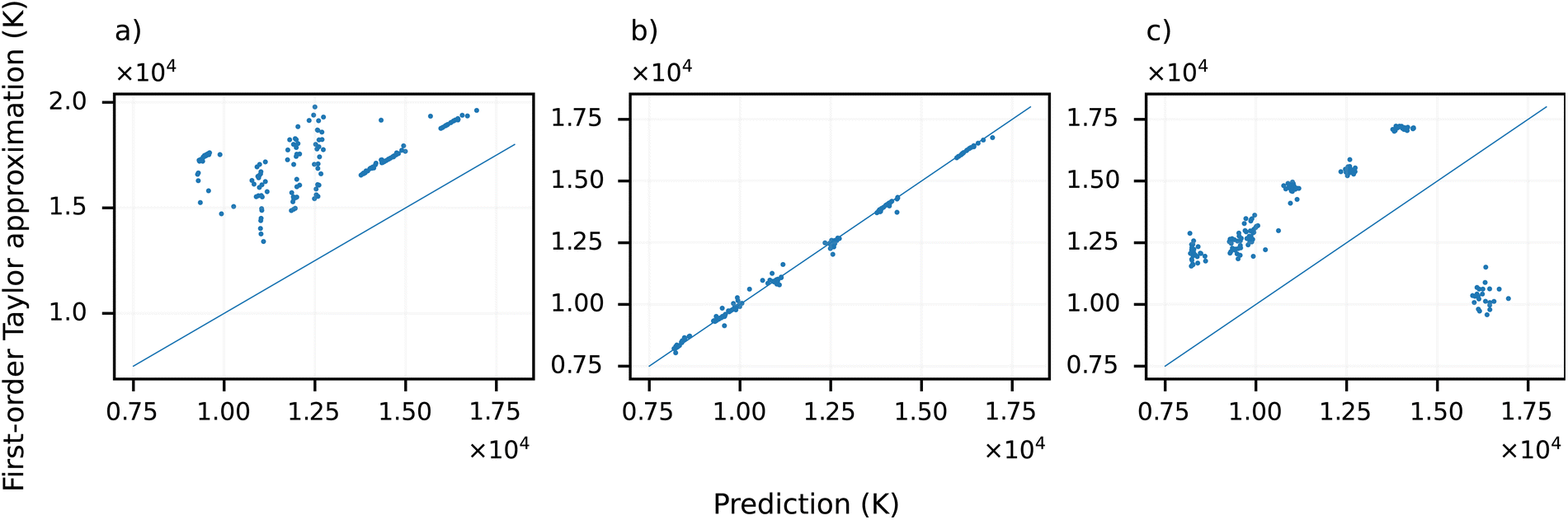Fig. 7 Comparison of the model prediction and its first order approximation (sum of the first two terms of the right-hand side of eqn (16)) for a single composition using three distinct root points for the Taylor decomposition: a) a prototype spectrum yielding a prediction of approximately zero; (b) the mean of the spectra corresponding to the same composition and temperature; and (c) a zero vector (which yields the base prediction of the model, i.e., approximately 10 000 K). The diagonal line represents a perfect correspondence, not a perfect prediction.

Fig. 8 (a) Detailed view of the 393.35 nm emission line in several spectra: the mean spectrum of the training dataset, the prototype spectra for 10⁴ and 1.6 × 10⁴ K, the mean relevance scores spectrum, and the mean Taylor spectrum. (b) Comparison of the trained models' prediction for a selected prototype spectrum and their baseline prediction. The horizontal line denotes the temperature for which the prototype spectrum was generated.

Moreover, several emission lines present in the prototype spectra appear or disappear in a step-wise manner: the emission line at 504.10 nm (corresponding to Fe I 504.10 nm and/or Si II 504.10 nm with corresponding upper energy levels of 3.4 and 12.5 eV, respectively) appears in prototype spectra corresponding to temperatures above 14 000 K (here only shown for 16 000 K in Fig. 6d). Other emission lines, such as 252.55 (Fe II 252.54 nm (11.1 eV) and/or Ti II 252.56 nm (5.0 eV)) and 393.35 nm (Ca II 393.36 nm (3.2 eV) and/or Fe I 393.35 (6.2 eV)), gradually decrease, eventually flipping around the prototype closest to the baseline prediction (10 000 K, Fig. 6a–c). Moreover, note the considerable potential spectral interference, which would invalidate the standard Boltzmann plot technique using these lines. Hence, provided with accurate ground truth values obtained using external measurements (decoupled from the LIBS emission spectra), ANNs could address some of the challenges faced by standard methods. The extent of the necessary external measurements required to train such ANNs applicable in practical settings is yet to be determined.

Considering the selective presence of the emission lines in the prototype spectra, perturbing these emission lines should only affect predictions in the temperatures where they are present. This is indeed the case, as shown in Fig. 9. Perturbing (setting equal to 0 in the spectrum) the emission lines at 504.16 (Fe I 504.10 nm (3.4 eV) and/or Si II 504.10 nm (12.5 eV)) and 637.14 nm (Si II 637.13 nm (10.1 eV) and/or Ti I 637.14 nm (4.1 eV)), which first appear in the prototype spectrum of 14 000 K affects the predictions only in the 14 000–18 000 K range. On the contrary, perturbing the emission lines at 252.55 (Fe II 252.54 nm (11.1 eV upper energy level) and/or Ti II 252.56 nm (5.0 eV)) and 393.35 nm (Ca II 393.36 nm (3.2 eV) and/or Fe I 393.35 nm (6.2 eV)), present in every prototype spectrum, affects every prediction. Moreover, there is a clear change in the dominant shift's direction caused by the removal of the considered emission lines. In the temperature range where the emission lines' intensities are negative in the corresponding prototype spectra, the lines' removal causes an upward shift in the predicted temperature, and vice versa in the case of positive intensities.

Fig. 9 Comparison of the predicted temperatures before and after perturbing the denoted emission line. The colors correspond to the highlighting used in Fig. 6 and 10 (both in ESI†). The diagonal lines denote perfect correspondence and their color is selected solely for the sake of visibility. The denoted wavelengths correspond to Fe II 252.54 nm (11.1 eV upper energy level) and/or Ti II 252.56 nm (5.0 eV); Ca II 393.36 nm (3.2 eV) and/or Fe I 393.35 nm (6.2 eV); Fe I 504.10 nm (3.4 eV) and/or Si II 504.10 nm (12.5 eV); and Si II 637.13 nm (10.1 eV) and/or Ti I 637.14 nm (4.1 eV).

Most emission lines deemed important by the ANN correspond to a convolution of multiple emission lines that cannot be resolved spectroscopically. Nevertheless, by analyzing the spectroscopic constants associated with these emission lines, it is possible to identify the strongest line with a high degree of confidence. Despite the order of magnitude higher concentration of Si in the considered targets, the ionic Si lines' upper energy levels are too high to exhibit notable intensity contribution to the observed composite emission features. Consequently, the ANN has been trained to prioritize emission lines from Fe and Ti, mirroring the approach frequently adopted by expert spectroscopists.

Nevertheless, while the emission line intensities in the prototype spectra are related to the corresponding intensities in the training spectra, they are not linearly correlated (Fig. 10c). Namely, the 393.35 nm emission line's intensity exhibits a good linear correlation between the prototype and emission spectra. On the other hand, the remaining three shown emission lines exhibit different behaviors: the 252.55 nm emission line shows a logarithmic dependence, while the 504.10 and 637.14 nm emission lines show an approximately binary relationship (that is, present or not present). Note that this comparison is done instead of considering the Boltzmann plot to avoid the impact of the changing composition in the training dataset. For example, the 504.10 nm emission line remains unchanged in the spectra corresponding to several temperatures. Accordingly, the line intensities in the corresponding prototype spectra are close to 0.

Fig. 10 (a) Mean spectrum of the training dataset and (b)–(e) relationship of the 4 highlighted emission lines' intensities in the temperature-wise mean spectrum and the prototype spectra. The full vertical and horizontal lines mark the mean intensity in the training and prototype spectra, respectively. The dashed lines denote the line intensity at the temperature which coincides with the baseline prediction of the model.

An apparent discrepancy exists between the relevance scores and the Taylor decomposition, attributable solely to the intrinsic formulations of these two methodologies. The relevance scores do not consider the sign of values, rendering them sign-agnostic. Consequently, averaging over different temperatures and/or compositions can lead cause the Taylor spectra to approach 0. On the contrary, the relevance scores are non-negative. Hence, averaging several relevance score spectra increases yields a spectrum with an enhanced signal-to-noise ratio, i.e., more pronounced emission lines. Overall, despite these methodological differences, all three approaches—when applied iteratively—yield qualitatively similar outcomes, consistently emphasizing the significance of the identified emission lines.

Our final comments on the interpretability technique using prototype spectra address the stability of the generated prototype spectra. Briefly, the obtained prototype spectra were found to be transferable between the distinct trained models, up to a constant error. In turn, this error was found to be linearly dependent on the models' baseline prediction (Fig. 8b). Thus, the prediction error on the prototype spectra resulting from transferring a prototype spectrum between models is linearly proportional to the value predicted from a zero vector (the base prediction).

4 Conclusions

This empirical study delves into the inner workings of artificial neural network (ANN) models employed to predict plasma temperature based on optical emission (LIBS) spectra. The investigation is carried out in a controlled manner using synthetic data with known ground truth. These efforts are to be extended to experimentally collected spectra in the future. To avoid propagating errors in temperature determination from the Boltzmann plot method, an external technique for temperature measurement will be used in future studies. The study employs three interpretability techniques to shed light on the ANN's behavior. Relevance scores showed a potential to investigate the model's behavior systematically: perturbing the variables found important via relevance scores resulted in a more pronounced impact on the model's prediction compared to the perturbation of intensity values with a low assigned relevance score. The stability of relevance scores across differently initialized models suggests that initialization has minimal impact on the learned approximation. Taylor decomposition-based analysis provides additional insights, namely about the non-linearity in the model. The Taylor decomposition showed better resolution but a strong dependence on the root point's choice. Lastly, the prototype spectra corresponding to specific temperatures contain a set of well-defined emission lines that exhibit distinct behaviors. Certain lines appear or disappear in a step-wise manner. Perturbing these lines affects predictions within specific temperature ranges, with a clear shift directionality depending on the emission lines' intensities. Overall, the results suggest that if trained on accurate ground truth values obtained via external measurements, ANNs could greatly enhance our capabilities to diagnose plasmas using their optical emission spectra. Moreover, the presented trends suggest that (with proper regularization on well-controlled synthetic spectra) the ANN learns spectroscopically sound trends in the data, which we can interpret and translate into domain expertise. This is crucial, because owing to the general approximation theorem, the ANNs could very well fit spurious correlations in the data, rendering any further efforts towards the improvement of laser-induced plasma temperature using ANNs futile. Most importantly, we present a set of robust techniques that can be used to probe and understand any ANNs developed and applied in the future. Nevertheless, the broader applicability of the determination of laser-induced plasma temperature using artificial neural networks in practical scenarios is yet to be established. A significant obstacle in this regard is ensuring the precision of experimental methodologies employed to derive ground truth values. In the spectrum of available methods, Rayleigh and Thomson scattering techniques are particularly noteworthy for their potential.

Author contributions

EK: led the conceptualization, visualization, and preparation of the original draft, laying the foundation for the study's theoretical framework and ensuring the manuscript's initial coherence and direction. EK, HS, VL: collaboratively conducted the formal analysis, investigation, and methodology analysis, and played a critical role in the manuscript's review and editing process, ensuring the research's accuracy and reproducibility. JV, PK, PP, MF, JK: provided substantial review and editing contributions, enhancing the manuscript's clarity, coherence, and overall quality through critical feedback and revisions. The project conceptualization and ongoing research activities, particularly in applying ANN for the evaluation of plasmophysical data. PP, MF, JK: were instrumental in funding acquisition, securing the financial support necessary for the research's execution and dissemination. JK, MF: supplied essential resources, facilitating the corresponding research.

Conflicts of interest

There are no conflicts to declare.

Acknowledgements

HS, VL, and MF would like to acknowledge the financial support of the Technology Agency of the Czech Republic (TAČR, NCK) under the grant under TN02000009/07 FREYA. PK and PP would like to acknowledge the financial support of the Czech Science Foundation (GACR) under grant number 23-05186K.

Notes and references

1. J. D. Winefordner, I. B. Gornushkin, T. Correll, E. Gibb, B. W. Smith and N. Omenetto, J. Anal. At. Spectrom., 2004, 19, 1061–1083.
2. V. Palleschi, ChemTexts, 2020, 6, 1–16.
3. A. Botto, B. Campanella, S. Legnaioli, M. Lezzerini, G. Lorenzetti, S. Pagnotta, F. Poggialini and V. Palleschi, J. Anal. At. Spectrom., 2019, 34, 81–103.
4. S. Legnaioli, B. Campanella, F. Poggialini, S. Pagnotta, M. Harith, Z. Abdel-Salam and V. Palleschi, Anal. Methods, 2020, 12, 1014–1029.
5. S. K. H. Shah, J. Iqbal, P. Ahmad, M. U. Khandaker, S. Haq and M. Naeem, Radiat. Phys. Chem., 2020, 170, 108666.
6. D. Santos Jr, L. C. Nunes, G. G. A. de Carvalho, M. da Silva Gomes, P. F. de Souza, F. de Oliveira Leme, L. G. C. dos Santos and F. J. Krug, Spectrochim. Acta, Part B, 2012, 71, 3–13.
7. R. S. Harmon, R. E. Russo and R. R. Hark, Spectrochim. Acta, Part B, 2013, 87, 11–26.
8. S. Sheta, M. S. Afgan, Z. Hou, S.-C. Yao, L. Zhang, Z. Li and Z. Wang, J. Anal. At. Spectrom., 2019, 34, 1047–1082.
9. A. Bengtson, Spectrochim. Acta, Part B, 2017, 134, 123–132.
10. C. Fabre, Spectrochim. Acta, Part B, 2020, 166, 105799.
11. P. R. Villas-Boas, M. A. Franco, L. Martin-Neto, H. T. Gollany and D. M. B. P. Milori, Eur. J. Soil Sci., 2020, 71, 805–818.
12. P. R. Villas-Boas, M. A. Franco, L. Martin-Neto, H. T. Gollany and D. M. B. P. Milori, Eur. J. Soil Sci., 2020, 71, 789–804.
13. F. Ruan, T. Zhang and H. Li, Appl. Spectrosc. Rev., 2019, 54, 573–601.
14. Z. Wang, M. Sher Afgan, W. Gu, Y. Song, Y. Wang, Z. Hou, W. Song and Z. Li, TrAC, Trends Anal. Chem., 2021, 143, 116385.
15. E. Képeš, J. Vrábel, J. El Haddad, A. Harhira, P. Pořízka and J. Kaiser, in Machine Learning in the Context of Laser-Induced Breakdown Spectroscopy, John Wiley & Sons, Ltd, 2023, ch. 15, pp. 305–330.
16. J. El Haddad, A. Harhira, E. Képeš, J. Vrábel, J. Kaiser and P. Pořízka, in Chemometric Processing of LIBS Data, John Wiley & Sons, Ltd, 2023, ch. 12, pp. 241–275.
17. E. Képeš, J. Vrábel, P. Pořízka and J. Kaiser, J. Anal. At. Spectrom., 2021, 36, 1410–1421.
18. G. Cristoforetti, A. De Giacomo, M. Dell'Aglio, S. Legnaioli, E. Tognoni, V. Palleschi and N. Omenetto, Spectrochim. Acta, Part B, 2010, 65, 86–95.
19. Z. Wang, L. Li, L. West, Z. Li and W. Ni, Spectrochim. Acta, Part B, 2012, 68, 58–64.
20. X. Li, Z. Wang, S.-L. Lui, Y. Fu, Z. Li, J. Liu and W. Ni, Spectrochim. Acta, Part B, 2013, 88, 180–185.
21. L. Li, Z. Wang, T. Yuan, Z. Hou, Z. Li and W. Ni, J. Anal. At. Spectrom., 2011, 26, 2274–2280.
22. J. Feng, Z. Wang, Z. Li and W. Ni, Spectrochim. Acta, Part B, 2010, 65, 549–556.
23. W. Gu, Z. Hou, W. Song, L. Li, X. Yu, J. Liu, Y. Song, M. Sher Afgan, Z. Li, Z. Liu and Z. Wang, Anal. Chim. Acta, 2022, 1205, 339752.
24. J. A. Aguilera and C. Aragón, Appl. Phys. A: Mater. Sci. Process., 1999, 69, S475–S478.
25. S. Yalçin, D. R. Crosley, G. P. Smith and G. W. Faris, Laser Applications to Chemical and Environmental Analysis, 1996, pp. LWA–2.
26. J. A. Aguilera and C. Aragón, Spectrochim. Acta, Part B, 2004, 59, 1861–1876.
27. A. Safi, S. H. Tavassoli, G. Cristoforetti, S. Legnaioli, V. Palleschi, F. Rezaei and E. Tognoni, J. Adv. Res., 2019, 18, 1–7.
28. J. A. Aguilera and C. Aragón, Spectrochim. Acta, Part B, 2007, 62, 378–385.
29. L. M. John, R. C. Issac, S. Sankararaman and K. K. Anoop, J. Anal. At. Spectrom., 2022, 37, 2451–2460.
30. S. Zhang, X. Wang, M. He, Y. Jiang, B. Zhang, W. Hang and B. Huang, Spectrochim. Acta, Part B, 2014, 97, 13–33.
31. A. Thorne, U. Litzén and S. Johansson, Spectrophysics: Principles and Applications, Springer Science & Business Media, 1999.
32. L. Pardini, S. Legnaioli, G. Lorenzetti, V. Palleschi, R. Gaudiuso, A. De Giacomo, D. Diaz Pace, F. Anabitarte Garcia, G. de Holanda Cavalcanti and C. Parigger, Spectrochim. Acta, Part B, 2013, 88, 98–103.
33. A. El Sherbini, H. Hegazy and T. M. El Sherbini, Spectrochim. Acta, Part B, 2006, 61, 532–539.
34. H. Saeidfirozeh, A. K. Myakalwar, P. Kubelík, A. Ghaderi, V. Laitl, L. Petera, P. B. Rimmer, O. Shorttle, A. N. Heays and A. Křivková, et al. , J. Anal. At. Spectrom., 2022, 37, 1815–1823.
35. J. Vrábel, E. Képeš, P. Pořízka and J. Kaiser, in Artificial Neural Networks for Classification, John Wiley & Sons, Ltd, 2022, ch. 9, pp. 213–240.
36. L. Brunnbauer, Z. Gajarska, H. Lohninger and A. Limbeck, TrAC, Trends Anal. Chem., 2023, 159, 116859.
37. C. Zhang, L. Zhou, F. Liu, J. Huang and J. Peng, Artif. Intell. Rev., 2023, 1–35.
38. L.-N. Li, X.-F. Liu, F. Yang, W.-M. Xu, J.-Y. Wang and R. Shu, Spectrochim. Acta, Part B, 2021, 180, 106183.
39. W. Zhao, C. Li, C. Yan, H. Min, Y. An and S. Liu, Anal. Chim. Acta, 2021, 1166, 338574.
40. E. Képeš, J. Vrábel, T. Brázdil, P. Holub, P. Pořízka and J. Kaiser, Talanta, 2024, 266, 124946.
41. A. Mahendran and A. Vedaldi, Proceedings of the IEEE Conference on Computer Vision and Pattern Recognition, 2015, pp. 5188–5196.
42. D. Erhan, Y. Bengio, A. Courville and P. Vincent, Visualizing higher-layer features of a deep network, University of Montreal, 2009, vol. 1341, p. 1.
43. F.-L. Fan, J. Xiong, M. Li and G. Wang, IEEE Trans. Radiat. Plasma Med. Sci., 2021, 5, 741–760.
44. Y. Zhang, P. Tiňo, A. Leonardis and K. Tang, IEEE Trans. Emerg. Top. Comput. Intell., 2021, 5, 726–742.
45. Q. Zhang and S. Zhu, Front. Inf. Technol. Electron. Eng., 2018, 19, 27–39.
46. F.-L. Fan, J. Xiong, M. Li and G. Wang, IEEE Trans. Radiat. Plasma Med. Sci., 2021, 5, 741–760.
47. R. C. Wiens, S. Maurice, B. Barraclough, M. Saccoccio, W. C. Barkley, J. F. Bell, S. Bender, J. Bernardin, D. Blaney and J. Blank, et al. , Space Sci. Rev., 2012, 170, 167–227.
48. S. Maurice, R. Wiens, M. Saccoccio, B. Barraclough, O. Gasnault, O. Forni, N. Mangold, D. Baratoux, S. Bender and G. Berger, et al. , Space Sci. Rev., 2012, 170, 95–166.
49. H. Sun, H. Chang, M. Rong, Y. Wu and H. Zhang, Phys. Plasmas, 2020, 27, 073508.
50. K. Dzierżega, A. Mendys and B. Pokrzywka, Spectrochim. Acta, Part B, 2014, 98, 76–86.
51. H. Zhang, Y. Wu, H. Sun, F. Yang, M. Rong and F. Jiang, Spectrochim. Acta, Part B, 2019, 157, 6–11.
52. H. Zhang, H. Sun, Y. Wu and Q. Zhou, Spectrochim. Acta, Part B, 2021, 177, 106103.
53. M. Cvejić, K. Dzierżęga and T. Pięta, Appl. Phys. Lett., 2015, 107, 024102.
54. I. Jolliffe and J. Cadima, Philos. Trans. R. Soc., A, 2016, 374, 20150202.
55. P. Pořízka, J. Klus, E. Képeš, D. Prochazka, D. W. Hahn and J. Kaiser, Spectrochim. Acta, Part B, 2018, 148, 65–82.
56. P. Geladi and B. R. Kowalski, Anal. Chim. Acta, 1986, 185, 1–17.
57. T. Mehmood, K. H. Liland, L. Snipen and S. Sæbø, Chemom. Intell. Lab. Syst., 2012, 118, 62–69.
58. C. Aragón and J. A. Aguilera, Spectrochim. Acta, Part B, 2008, 63, 893–916.
59. A. Ciucci, M. Corsi, V. Palleschi, S. Rastelli, A. Salvetti and E. Tognoni, Appl. Spectrosc., 1999, 53, 960–964.
60. E. Tognoni, G. Cristoforetti, S. Legnaioli, V. Palleschi, A. Salvetti, M. Mueller, U. Panne and I. Gornushkin, Spectrochim. Acta, Part B, 2007, 62, 1287–1302.
61. N. Konjević, Phys. Rep., 1999, 316, 339–401.
62. C. M. S. Laboratory, ChemCam on Mars, online, 2022, https://www.msl-chemcam.com/, accessed: 2022-11-02.
63. A. Kramida, Y. Ralchenko, J. Readeret al., NIST Atomic Spectra Database (Ver. 5.2)[Online], 2014.
64. S. Sahal-Bréchot, M. S. Dimitrijević, N. Moreau and N. B. Nessib, Adv. Space Res., 2014, 54, 1148–1151.
65. S. Sahal-Bréchot, M. Dimitrijević, N. Moreau and N. B. Nessib, Phys. Scr., 2015, 90, 054008.
66. STARK-B., Available online: http://stark-b.obspm.fr, accessed on 12 July 2020.
67. M. Ferus, P. Kubelík, L. Petera, L. Lenža, J. Koukal, A. Křivková, V. Laitl, A. Knížek, H. Saedfirozeh, A. Pastorek, T. Kalvoda, L. Juha, R. Dudžák, S. Civiš, E. Chatzitheodoridis and M. Krůs, Astron. Astrophys., 2019, 630, A127.
68. E. Tognoni and G. Cristoforetti, Opt Laser. Technol., 2016, 79, 164–172.
69. J.-M. Mermet, P. Mauchien and J.-L. Lacour, Spectrochim. Acta, Part B, 2008, 63, 999–1005.
70. J. Klus, P. Pořízka, D. Prochazka, J. Novotný, K. Novotný and J. Kaiser, Spectrochim. Acta, Part B, 2016, 126, 6–10.
71. E. Képeš, P. Pořízka and J. Kaiser, J. Anal. At. Spectrom., 2019, 34, 2411–2419.
72. M. D. Dyar, S. Giguere, C. Carey and T. Boucher, Spectrochim. Acta, Part B, 2016, 126, 53–64.
73. E. Képeš, P. Pořízka, J. Klus, P. Modlitbová and J. Kaiser, J. Anal. At. Spectrom., 2018, 33, 2107–2115.
74. F. Gan, G. Ruan and J. Mo, Chemom. Intell. Lab. Syst., 2006, 82, 59–65.
75. P. Yaroshchyk and J. E. Eberhardt, Spectrochim. Acta, Part B, 2014, 99, 138–149.
76. P. Mehta, M. Bukov, C.-H. Wang, A. G. Day, C. Richardson, C. K. Fisher and D. J. Schwab, Phys. Rep., 2019, 810, 1–124.
77. K. Hornik, M. B. Stinchcombe and H. L. White, Neural Networks, 1989, 2, 359–366.
78. M. A. Nielsen, Neural Networks and Deep Learning, Determination press, San Francisco, CA, USA, 2015, vol. 25.
79. T. Szandała, in Review and Comparison of Commonly Used Activation Functions for Deep Neural Networks, 2021, pp. 203–224.
80. A. L. Maas, A. Y. Hannun and A. Y. Ng, Rectifier Nonlinearities Improve Neural Network Acoustic Models, Proceedings of the 30th International Conference on Machine Learning, 2013, vol. 28, p. 3.
81. K. Yuan, B. Ying, S. Vlaski and A. H. Sayed, 2016 IEEE 26th International Workshop on Machine Learning for Signal Processing, MLSP, 2016, pp. 1–6.
82. L. Bottou, International Conference on Computational Statistics, 2010.
83. S. Ruder, An Overview of Gradient Descent Optimization Algorithms, 2017.
84. E. M. Dogo, O. J. Afolabi, N. I. Nwulu, B. Twala and C. O. Aigbavboa, 2018 International Conference on Computational Techniques, Electronics and Mechanical Systems, CTEM, 2018,pp. 92–99.
85. S. Wager, S. Wang and P. S. Liang, Advances in Neural Information Processing Systems, 2013, vol. 26.
86. P. Baldi and P. J. Sadowski, Advances in Neural Information Processing Systems, 2013, vol. 26.
87. D. Kingma and J. Ba, International Conference on Learning Representations, 2014.
88. M. Abadi, A. Agarwal, P. Barham, E. Brevdo, Z. Chen, C. Citro, G. S. Corrado, A. Davis, J. Dean, M. Devin, S. Ghemawat, I. Goodfellow, A. Harp, G. Irving, M. Isard, Y. Jia, R. Jozefowicz, L. Kaiser, M. Kudlur, J. Levenberg, D. Mané, R. Monga, S. Moore, D. Murray, C. Olah, M. Schuster, J. Shlens, B. Steiner, I. Sutskever, K. Talwar, P. Tucker, V. Vanhoucke, V. Vasudevan, F. Viégas, O. Vinyals, P. Warden, M. Wattenberg, M. Wicke, Y. Yu and X. Zheng, TensorFlow: Large-Scale Machine Learning on Heterogeneous Systems, 2015, https://www.tensorflow.org/.
89. F. Chollet, Keras, https://github.com/fchollet/keras, 2015.
90. G. Van Rossum and F. L. Drake, Python 3 Reference Manual, CreateSpace, Scotts Valley, CA, 2009.
91. G. Montavon, W. Samek and K.-R. Müller, Digital signal processing, 2018, vol. 73, pp. 1–15.
92. J. Khan, J. S. Wei, M. Ringnér, L. H. Saal, M. Ladanyi, F. Westermann, F. Berthold, M. Schwab, C. R. Antonescu, C. Peterson and P. S. Meltzer, Nat. Med., 2001, 7, 673–679.
93. J. M. Zurada, A. Malinowski and I. Cloete, Proceedings of IEEE International Symposium on Circuits and Systems-ISCAS;94, 1994, pp. 447–450.
94. A. H. Sung, Expert Syst. Appl., 1998, 15, 405–411.
95. E. Képeš, J. Vrábel, O. Adamovsky, S. Střítežská, P. Modlitbová, P. Pořízka and J. Kaiser, Anal. Chim. Acta, 2022, 1192, 339352.
96. I. E. Nielsen, D. Dera, G. Rasool, R. P. Ramachandran and N. C. Bouaynaya, IEEE Signal Process. Mag., 2022, 39, 73–84.
97. G. Montavon, S. Bach, A. Binder, W. Samek and K.-R. Müller, Proceedings of the ICML 2016 Workshop on Visualization for Deep Learning, 2016.
98. S. Bazen, X. Joutard and B. Magdalou, Journal of Economic and Social Measurement, 2017, 42(2), 101–121,  DOI:10.3233/JEM-170439 , https://content.iospress.com/articles/journal-of-economic-and-social-measurement/jem439.
99. S. Bach, A. Binder, G. Montavon, F. Klauschen, K.-R. Müller and W. Samek, PLoS One, 2015, 10, e0130140.
100. J. Yosinski, J. Clune, A. Nguyen, T. Fuchs and H. Lipson, arXiv, 2015, preprint, arXiv:1506.06579,  DOI:10.48550/arXiv.1506.06579.
101. K. Simonyan, A. Vedaldi and A. Zisserman, arXiv, 2013, preprint, arXiv:1312.6034,  DOI:10.48550/arXiv.1312.6034.

---

Footnote

† Electronic supplementary information (ESI) available. See DOI: https://doi.org/10.1039/d3ja00363a

---