
On-line vacuum degree monitoring of vacuum circuit breakers based on laser-induced breakdown spectroscopy combined with random forest algorithm
Feilong
Zhang
,
Huan
Yuan
 *,
Aijun
Yang
*,
Xiaohua
Wang
,
Jifeng
Chu
,
Dingxin
Liu
and
Mingzhe
Rong
*,
Aijun
Yang
*,
Xiaohua
Wang
,
Jifeng
Chu
,
Dingxin
Liu
and
Mingzhe
Rong
School of Electrical Engineering, Xi'an Jiaotong University, Xi'an, 710049, China. E-mail: huanyuan@xjtu.edu.cn
First published on 22nd November 2023
Abstract
The present study introduces a novel method for online vacuum monitoring of vacuum circuit breakers, which overcomes the limitations of conventional offline monitoring methods in engineering applications. Specifically, the proposed method uses laser-induced breakdown spectroscopy (LIBS) in combination with the random forest (RF) algorithm to monitor the vacuum level of the breaker. The experimental setup included the selection spectral lines from four elements (one in the target material and three in the ambient gas). Spectral data were collected using the LIBS platform under various pressure conditions ranging from 10−3 Pa to 105 Pa. An RF model was established to classify the pressure level using spectral data. The classification performance is tested with a confusion matrix. We employed various spectral preprocessing techniques to enhance the distinctiveness of spectral features. The choice of the optimal preprocessing method was determined by assessing the correlation coefficient (R2) and root mean square error (RMSE), resulting in improved accuracy in vacuum level classification. The variable importance random forest (VIRF) algorithm was also employed for feature selection on the raw spectra to eliminate redundant information, thus enhancing the model's efficiency and accuracy. Utilizing out-of-bag (OOB) error as the evaluation metric, we systematically explored the impact of decision tree quantity (ntree) and the number of selected features (mtry) on the model's performance, optimizing it to its highest performance. The results indicate that the proposed method can achieve an accuracy of over 99% of vacuum classification, comparable to traditional offline vacuum monitoring technology. This demonstrates that LIBS technology combined with the RF algorithm represents a promising new approach for online vacuum monitoring of vacuum circuit breakers.
1. Introduction
Vacuum circuit breakers are increasingly being utilized in medium voltage fields, replacing oil and SF6 circuit breakers due to their high arc extinguishing capacity, compact structure, and environmental friendliness.1–3 Maintaining the appropriate vacuum level within the vacuum interrupter is critical for the reliable operation of vacuum circuit breakers. According to the Chinese power industry standard “Technical Conditions for Ordering High-Voltage Vacuum Circuit Breakers (12 kV–40.5 kV)” (DL/L 403-2000), the gas pressure in the vacuum interrupter chamber should remain below 6.6 × 10⁻² Pa.4 However, factors such as contact bounce, mechanical collisions, flange damage, and bellows aging can lead to a reduction in the vacuum level during the operation of vacuum circuit breakers. In the manufacturing of vacuum circuit breakers, the process involves a high-temperature firing stage at 800 °C, which extends over a considerable duration to achieve integral formation. Consequently, measuring vacuum levels can only be done through external means. Currently, there are two major methods for detecting vacuum levels available in the market: offline and online testing. Offline detection methods, such as frequency withstand voltage and magnetron discharge, represent a relatively mature technology.5 However, they require the equipment to be taken offline, resulting in economic losses. The offline detection methods are better suited for testing vacuum circuit breakers during production but are not suitable for practical engineering applications. The only two online monitoring methods (partial discharge method and shield cage potential method) have relatively high detection limits and are susceptible to various electromagnetic pulses within the power system, leading to misjudgments.6–8 Therefore, there is a critical need for a reliable online monitoring system for vacuum circuit breakers. Furthermore, the measurement of vacuum levels represents a major obstacle to the widespread adoption of high-voltage vacuum switches in power transmission systems.LIBS is an atomic emission spectroscopy technique that employs laser-induced plasma to analyze the elemental composition of materials.9 LIBS has demonstrated excellent potential for qualitative and quantitative analysis,11 with advantages including rapid, field-ready analysis, remote monitoring, high sensitivity, no need for complex sample preparation, almost no damage to the sample, and multi-element study compared to traditional analytical techniques.12 Consequently, LIBS has seen a rapid development over the last two decades and has found applications in various fields including environmental testing,10,13 biomedicine,14,15 metallurgical analysis,16–18 military applications,14,19 space exploration,20,21 and scientific and technological archaeology,22 among others.
Scholars worldwide have conducted extensive research on the radiative properties of laser-induced plasmas and characteristic parameters of spectra under varying gas pressures.35–37 Experimental studies have shown significant impacts of ambient pressure on the plasma formation process, including plasma morphology, signal intensity of emission spectra, spectral line broadening, signal-to-noise ratios, and target material ablation extent.
S. S. Harilal and colleagues at the Atlantic Northwest National Laboratory in the United States38 investigated laser-induced plasmas under conditions of 10−5 Torr (approximately 1.33 × 10⁻³ Pa), 10−2 Torr, 10 Torr, 300 Torr, and 760 Torr (approximately 105 Pa). The experiments revealed substantial differences in spectral radiative properties, with stark line broadening, signal-to-noise ratios, and plasma expansion characteristics among the five pressure levels. This further emphasizes the undeniable influence of ambient pressure on plasma generation and characteristic spectral parameters within the range from 10−5 Torr to one atmosphere.
Annemie Bogaerts and her team at the University of Antwerp39 developed a laser-induced plasma simulation model to investigate the interaction between laser radiation and solid target materials, as well as the effects of pressure on characteristic parameters such as plasma temperature, density, and expansion velocity during the plasma expansion process. Simulation results indicate a significant increase in plasma temperature and density at atmospheric pressure compared to vacuum conditions.
Our research group has pioneered the application of LIBS technology in the field of vacuum level detection and has been researching its potential for online vacuum monitoring in vacuum circuit breakers for several years. The underlying principle is based on employing pulsed laser to induce plasma on the surface of a metallic shield housed within the vacuum interrupter chamber of a vacuum circuit breaker. The resulting plasma exhibits a temporal scale on the order of nanoseconds and a spatial scale of sub-millimeters. Subsequently, an evaluation of the vacuum level is performed through the analysis of plasma morphology features and spectral characteristics. In a study, researchers investigated variations in the spectra of four elements (Cu, H, N, and O) at different air pressures. They employed the spectral intensity ratio method as an online monitoring system to determine the vacuum level.23 Subsequent research in 2017 demonstrated that the spectrum could serve as a characteristic quantity for assessing the vacuum degree.24 In 2018, further research confirmed the feasibility of using LIBS spectroscopy for vacuum degree detection at the microscopic scale. The researchers proposed a segmented feature extraction method using three metrics (distance between the target and the plasma center of mass, integrated intensity of the plasma spectral line, and plasma plume length) to distinguish between different pressure ranges, from 10−2 Pa to 105 Pa for the vacuum level.25 In our 2022 study, we verified that laser induced plasma has good stability and repeatability, further confirming the feasibility of the vacuum level detection method for vacuum switches using the LIBS technique.26 Despite the promising results, this method still requires further improvement in terms of efficiency, accuracy, and anti-interference capability of the feature extraction algorithm to address complex working conditions in future practical applications.
In recent years, various machine learning algorithms have been combined with LIBS techniques for quantitative and qualitative analysis in different fields. For instance, the combination of LIBS and support vector machines (SVM) has been employed to identify and classify polyvinyl chloride polymers.27 LIBS coupled with partial least squares (PLS) has been utilized for quantitative analysis of iron ore species.28 However, PLS, as a linear model, exhibits limited generalization capacity in nonlinear scenarios. SVM and convolutional neural network (CNN) algorithms are susceptible to overfitting when dealing with small sample sizes. To address these issues, the RF algorithm has been proposed as a new multi-classifier-based classification algorithm.29 Tang et al. used the LIBS technique combined with VIRF to classify different slag samples and achieved better performance than PLS and SVM models.16 Zhan et al. proposed LIBS combined with RF for fast classification of aluminum alloys and achieved an average accuracy of 98.45%.30 Wang et al. used the LIBS technique combined with VIRF for fast quantitative analysis of iron ore acidity, which showed better prediction performance than PLS and least squares support vector machine (LS-SVM) models.31 Feng et al. proposed a method for LIBS combined with RF to predict the contamination indicators of elemental Cu in atmospheric deposition samples, which showed excellent prediction performance with mean relative standard deviations (RSDs) of the prediction sets for the three contamination indicators ranging from 0.71% to 5.78%.32 These studies demonstrate the potential of employing LIBS in conjunction with RF as an effective approach for classification and quantitative analysis in diverse fields.
This study aims to validate the feasibility of using the RF algorithm based on LIBS spectral data for real-time monitoring of vacuum levels in circuit breakers. We established a LIBS experimental platform and collected 180 samples of elemental spectral lines under different pressure conditions. Evaluating using the R2 and RMSE, we determined the optimal preprocessing method for LIBS spectra. Subsequently, we applied the VI-RF algorithm to enhance model efficiency and accuracy. With an optimized model, we achieved an accuracy of over 99%, reaching the level of existing offline vacuum level detection methods in the market.
What sets our research apart from previous studies is its innovativeness in several key aspects: (1) we achieved higher accuracy under low vacuum conditions, particularly during the initial stages of gas leakage when early warnings are crucial. This innovation enables the timely detection of leaks in low vacuum situations. (2) Unlike prior research that relied on manually selected integral intensities of a few elemental spectral lines as features, our study used the raw spectral data as input. We employed a variable importance selection algorithm to automatically filter features, eliminating low-information spectra. This approach improved classification accuracy and reduced computation time, resulting in faster and more accurate responses. (3) Our research placed a strong emphasis on the raw spectral data and investigated multiple spectral preprocessing methods to enhance the distinctiveness of spectra at different vacuum levels. This adaptability of the algorithm model makes it better suited for vacuum level classification applications.
In summary, we propose a method for real-time monitoring of vacuum levels in circuit breakers using LIBS and the VIRF algorithm, which holds the potential to improve the reliability and efficiency of vacuum circuit breakers.
2. Experimental
Fig. 1 depicts a laboratory-built LIBS vacuum inspection system, featuring an Nd:YAG active electro-optic modulated Q laser (Dawa 300, Beamtech, Beijing). The laser is equipped with a 1 ns pulse width, an excitation wavelength of 1064 nm, and operates at a repetition rate of 5 Hz, delivering a laser pulse energy of 30 mJ for excitation. The laser beam is directed through a reflector and a lens, and subsequently passes through the glass incidence window into the vacuum cavity, then focuses on the copper target's surface. As a complement, the copper target was placed on a two-dimensional moving platform shown in Fig. 1b. The lens's focusing distance is adjusted to regulate the size of the focal spot.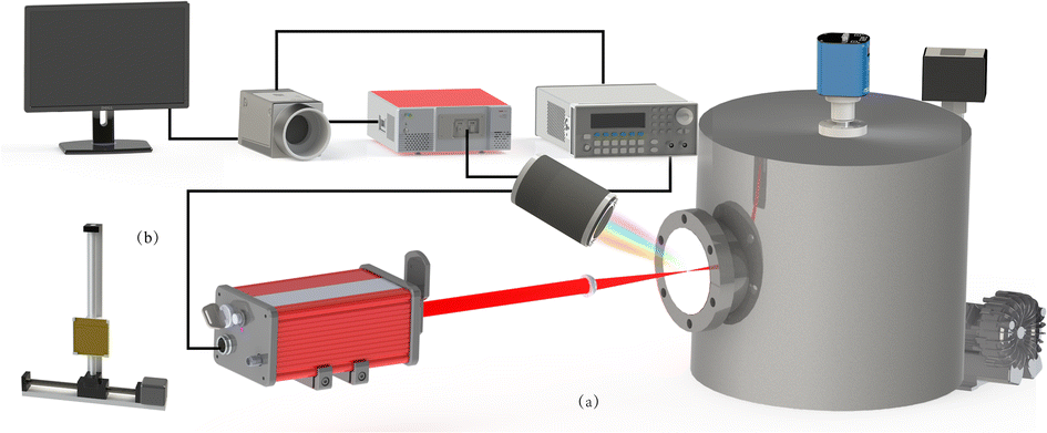 | ||
| Fig. 1 Illustration of the LIBS experimental setup for vacuum classification (a) and schematic of the two-dimensional movable platform for copper target placement (b). | ||
The copper target is positioned on a two-dimensional movable platform, containing 99.95% Cu and 0.05% impurities. The impurity elements include Zn, Mn, P, Ni, Sb, Al, Sn, Fe, etc. This is also the same material chosen as the shielding cover. The plasma excited by this process is collected by the lens through the viewing window into a conducting fiber and transmitted to a spectrometer (Aryelle Butterfly, Germany) for signal conversion and recording the raw spectral data by ICCD camera (Andor, England). A time delay system was used to control the time interval between laser emission and spectrometer signal acquisition. After several experimental comparisons, 200 ns delay time, 100 ns gate width, and 500 gain were obtained as the optimal parameters. In this case the best spectral signal-to-noise ratio can be obtained.
In manufacturing of vacuum circuit breakers, the process involves a high-temperature firing stage at 800 °C, which extends over a considerable duration to achieve integral formation. Consequently, measuring vacuum levels can only be done through external means. When establishing our experimental platform, we considered the inability to measure the vacuum levels within the vacuum interrupter without compromising its structural integrity. Even when employing prefabricated vacuum interrupter units for spectral data collection, it remains impossible to determine the vacuum level at which the collected spectra were obtained. Therefore, we chose to construct a vacuum chamber experimental setup to sample and record elemental spectra at different vacuum levels. This dataset serves as the foundation for training our algorithm model.
A vacuum system is employed to manage and manipulate the air pressure within the chamber, thereby simulating various levels of vacuum degradation. This system incorporates a turbomolecular pump and an ion pump along with several valves to regulate and control the pressure. For vacuum degree measurements in this experiment, a compound vacuum meter comprising a resistance vacuum meter and a hot cathode ionization vacuum meter was used. This meter is capable of measuring a range from 5 × 10⁻⁵ Pa to 1 × 10⁵ Pa, ensuring that the internal pressure within the vacuum chamber is maintained at the desired level.
To minimize the impact of randomness in the experiment and prevent interference from ablation pits at specific locations in subsequent experiments, we selected five different sites on the target for LIBS spectral acquisition in each group. The spectra of four elements (Cu in the target material, N, O, and H in the ambient gas elements) were collected at each vacuum level. This resulted in a total of 180 raw spectra acquired at nine different vacuum levels (ranging from 10−3 Pa to 105 Pa). The vacuum levels tested included 10−3 Pa, 10−2 Pa, 10−1 Pa, 1 Pa, 10 Pa, 102 Pa, 103 Pa, 104 Pa, and 105 Pa. For the construction of the RF model, we used 126 sets of spectra and corresponding vacuum level labels as the training set, while the remaining 54 sets were employed as the test set.
3. Methodology
3.1 Spectral pretreatment methods
In the experiment, uncertainties stemming from instrument variability, environmental noise, and matrix effects can exert an impact on the stability of the relationship between vacuum levels and spectral line intensities in LIBS quantitative analysis. Furthermore, a comprehensive spectroscopic analysis reveals the significant presence of background information and noise surrounding the analysis lines within the LIBS spectra. Therefore, it is essential to utilize appropriate LIBS spectral preprocessing methods to process the raw spectra, ultimately achieving exceptional classification performance.To enhance the classification performance of the RF model in this experiment, various preprocessing methods were applied. These included the first-order derivative (D1st) method, the wavelet transform method, multiple scattering correction (MSC), and standard normalization (SNV) for preprocessing the LIBS spectra. Multiple scattering correction was used to mitigate the influence of inhomogeneous particle distribution and particle size on the target surface, while standard normalization aimed to alleviate the effects of scattering, optical range transformation, particle distribution, and other factors on the target surface. In parallel, these techniques were employed to better highlight the distinctions among spectra at different vacuum levels. Concerning the RF algorithm, diverse data is indeed pivotal to the model's generalization capabilities, ensuring it can accurately classify new data. For instance, the first-order derivative emphasizes the slope information of spectra, SNV helps mitigate intensity variations, MSC corrects baseline drift, and wavelet transformation captures changes in various frequency domains. These preprocessing methods indeed aided in enhancing the distinctiveness among spectra at different vacuum levels.
The effects of pretreatment are evaluated using the RMSE and R2. The RMSE characterizes the deviation of the vacuum level calculated by the model from the actual value, while the R2 indicates the degree of interpretation of the vacuum level by the spectral data in the model. The optimal number of smoothing points is determined based on the balance between the two evaluation indexes:
 | (1) |
 | (2) |
3.2 Random forest algorithm
RF is a machine learning algorithm that combines multiple classification and regression trees using the Bagging method of ensemble learning. The algorithm creates a training set by randomly sampling the original dataset with replacement (known as bootstrap resampling) to perform classification analysis. Within each bootstrap sample, the relationship between spectral line intensities and vacuum levels is integrated to construct a random forest model. During classification, the algorithm combines the results of all trees and selects the class with the most votes as the final output.The construction of a random forest model typically involves four steps, as follows:
(1) A sample size of N is drawn from the original data with replacement N times, creating a subset of N samples. These samples serve as the input for the root node of the decision tree and are used to train a decision tree.
(2) From the M features in the sample, m features (where m ≪ M) are selected to minimize information entropy increase. The feature with the best classification ability is chosen, and the samples are divided into two groups based on the threshold value of this feature, forming a binary tree branch.
(3) The splitting process in step 2 continues until the node is not divisible, and there is no pruning throughout the entire decision tree formation process.
(4) Steps 1–3 are repeated N times to construct a random forest model with N decision trees. The process is illustrated in Fig. 2.
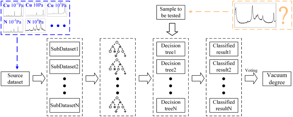 | ||
| Fig. 2 Flowchart of vacuum classification RF algorithm with spectra as input. | ||
Random forest is advantageous over other supervised learning algorithms due to its dual randomness. The first source of randomness is achieved by constructing different decision trees with put-back selection, ensuring randomness in data sample sampling. The second source is the random sampling of features, which provides randomness in the data feature piece. The dual randomness increases the variability of each tree, making random forest less susceptible to overfitting and providing good noise immunity.
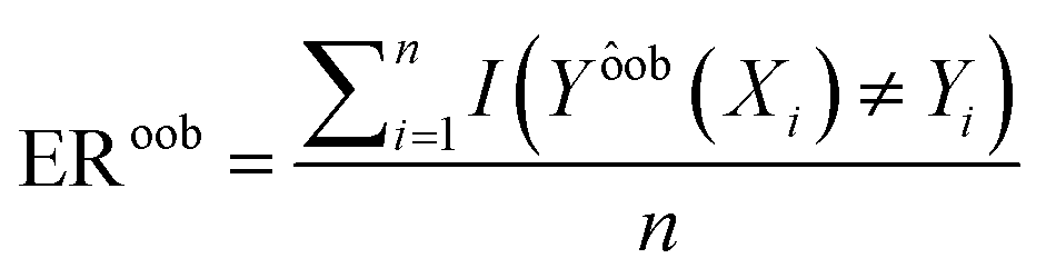
Another significant advantage of RF is that unbiased estimates of error can be obtained without the need for cross-validation or an independent test set. The quality of the model can be measured through internal evaluation of the error. In step 1, the remaining samples that are not included in the training set make up the test set. The probability that a model has not appeared in all training sets can be calculated using the following formulae:33
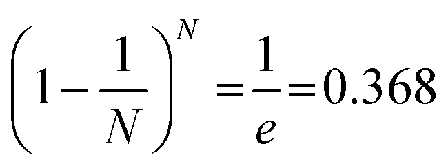 | (3) |
 | (4) |
Formula (1) illustrates that for N training sets, when randomly selecting N samples, there is a 36.8% chance that none of them will be chosen at least once. These unselected samples are referred to as out-of-bag (OOB) samples, which can be utilized to assess the model's generalization capability.
OOB error is an unbiased estimate of the generalization error of the random forest model, approximating the k-fold cross-validation method that requires significant computational resources. The OOB error is used as an evaluation metric in the optimized RF vacuum classification model to classify vacuum degrees of different samples. In decision trees, all input spectral samples are used as the root nodes of the decision tree, with peak intensity of spectral lines of the main component elements (such as Cu of the target material, and N, O, and H of the ambient gas) serving as feature quantities for post-judgment classification. Nodes are continuously branched layer by layer until non-divisible leaf nodes are obtained, which serve as the classification results.
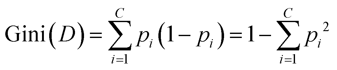
Decision trees are a popular tool for solving classification and regression problems. In constructing decision trees, the goal is to split the data into subsets that are as homogeneous as possible. A widely used measure of homogeneity is entropy. The ID3 and C4.5 algorithms use entropy to calculate the information gain and gain ratio, respectively, to determine which feature to split at each node. However, these algorithms can suffer from a bias towards features with many possible values. To address this issue, the classification and regression trees (CART) algorithm calculates the Gini coefficient as a measure of impurity. The Gini coefficient measures the probability of incorrectly classifying a randomly chosen sample if it were randomly labeled based on the distribution of classes in the node. The feature that minimizes the Gini coefficient is selected for splitting. The Gini coefficient is calculated using the following formula:
 | (5) |
Compared with ID3 and C4.5, the CART algorithm does not require pruning to correct for overfitting and only performs binary classification on nodes. All possible tree structures are directly compared using all available data, resulting in higher accuracy and computational efficiency.
The spectral sample serves as the root node of the decision tree, and the peak intensity of spectral lines corresponding to elements in the environment and target material is used as the feature variable for branching. Fig. 3 illustrates one of the decision trees generated by the model. In this tree, the initial branching condition is based on the spectral line intensity of N 442.2 nm. Samples with intensities below 621 a.u. are classified as vacuum degrees less than or equal to 102 Pa, while those with intensities above are categorized as vacuum degrees greater than or equal to 103 Pa. The decision tree is constructed by iteratively branching with different feature variables until each leaf node becomes indivisible. Regarding the final classification results for vacuum levels, it was observed that only the last sample in the last branch was inaccurately classified, wherein a group of spectral samples initially associated with a vacuum level of 0.1 Pa were erroneously classified as 1 Pa.
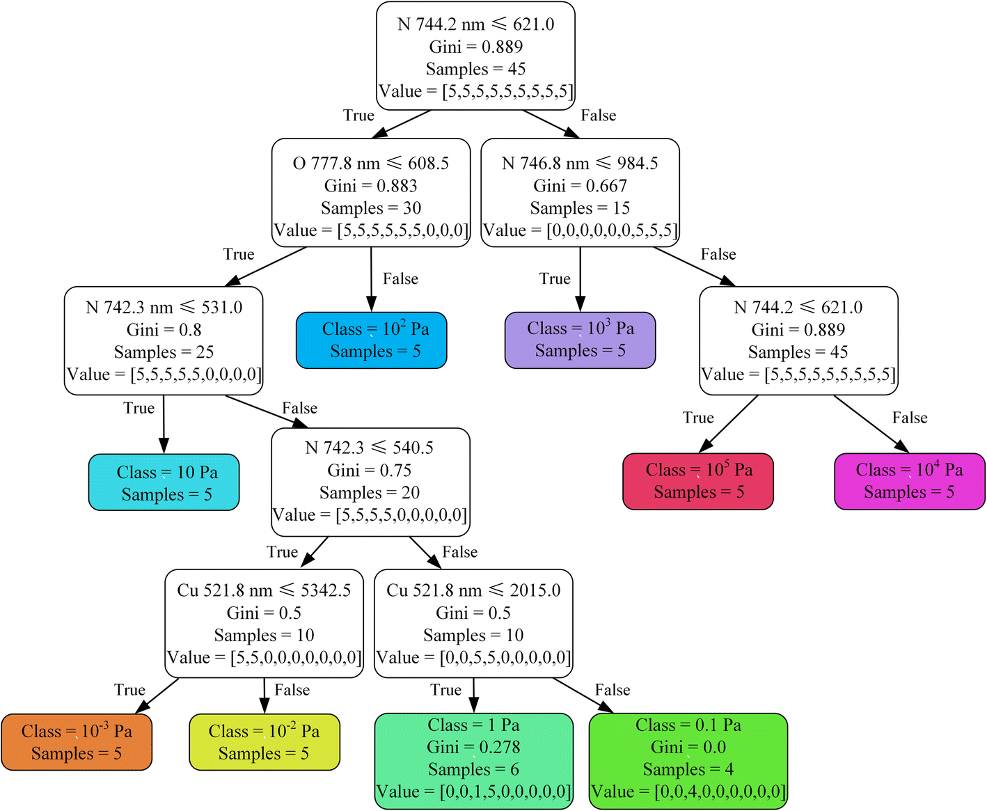 | ||
| Fig. 3 Vacuum classification result of one decision tree in the RF model. | ||
4. Results and discussion
4.1 LIBS spectral analysis
Fig. 4 displays the raw LIBS spectra acquired under different vacuum environments, ranging from 10−3 Pa to 105 Pa (10−3 Pa, 10−2 Pa, 10−1 Pa, 1 Pa, 10 Pa, 102 Pa, 103 Pa, 104 Pa, and 105 Pa). The spectra contain characteristic spectral lines of four elements: Cu, N, O, and H, which are from the target materials and the primary elements in the ambient gas in this experiment. By utilizing the National Institute of Standards and Technology (NIST) database34 to identify these four elements, it is observed that their characteristic spectral lines (Cu: 515.3 nm, 521.8 nm; N: 742.3 nm, 744.2 nm, 746.8 nm; O: 777.2 nm, 777.8 nm; H: 656.2 nm) exhibit different intensity levels under different atmospheric pressure environments.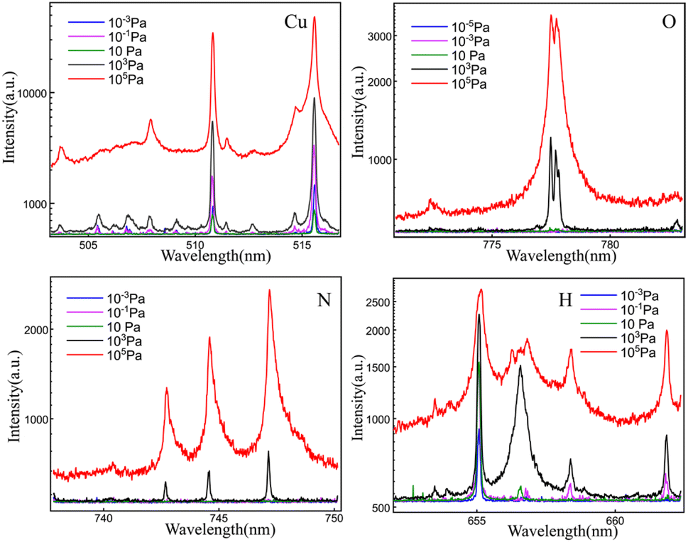 | ||
| Fig. 4 Vacuum chamber LIBS system collected original spectra of different elements at various pressures. | ||
A more intuitive observation reveals that, overall, the spectral line intensities of the four elements exhibit a monotonic relationship with pressure levels. With increasing pressure, the integrated spectral line intensities demonstrate an increasing trend. Notably, copper, as one of the target elements, exhibits differences compared to the other three gas-phase elements. Below 10 Pa, the spectral line intensity of copper experiences a slight decrease as pressure increases. This is attributed to the significantly increased mean free path between the plasma formed by the target material and the environmental air elements at lower pressures, resulting in minimal influence from the ambient pressure. From 10 Pa to 104 Pa, the spectral line intensity of copper sharply rises due to the increasing restrictive effect of environmental gases on the plasma, leading to intensified particle collisions within the plasma. However, when the pressure reaches 105 Pa, the spectral lines show a declining trend, while the three environmental gas elements continue to rise. This is because the plasma experiences strong shielding effects from the environmental gases, resulting in the attenuation of laser energy at the target material's surface and reduced target material ablation.
From this trend, it can be inferred that using spectral intensities as raw data enables the classification of the environmental pressure level at which the spectrum was excited through a random forest algorithm.
4.2 Classification performance of the RF model for vacuum levels
In this section, we present a comprehensive analysis of the classification performance of the random forest model for vacuum level prediction. The assessment is based on a meticulous evaluation of its ability to correctly classify and predict different vacuum levels.The confusion matrix plays a pivotal role in assessing the performance of the random forest model in vacuum level classification by providing a detailed breakdown of true positives, true negatives, false positives, and false negatives, enabling a comprehensive evaluation of the model's classification accuracy and error rates.
By collecting raw spectra and annotating them with corresponding vacuum level labels (10−3 Pa, 10−2 Pa, 10−1 Pa, 1 Pa, 10 Pa, 102 Pa, 103 Pa, 104 Pa, and 105 Pa), we established the original dataset. We constructed a random forest algorithm using a 7![[thin space (1/6-em)]](https://www.rsc.org/images/entities/char_2009.gif) :3 split ratio to create a training set and a test set. We employed repeated k-fold cross-validation with random partitions of the training and test sets to enhance model performance stability and mitigate the influence of random data partitioning. The visual representation of the generated confusion matrix is presented in the following figure.
:3 split ratio to create a training set and a test set. We employed repeated k-fold cross-validation with random partitions of the training and test sets to enhance model performance stability and mitigate the influence of random data partitioning. The visual representation of the generated confusion matrix is presented in the following figure.
From Fig. 5, it can be observed that the model exhibits excellent classification performance for vacuum levels above 10 Pa. However, the classification performance deteriorates for vacuum levels at or below 10−1 Pa. In the case of 10−1 Pa, it exhibits the poorest performance with only 34 samples correctly classified. There are 19 samples misclassified as 10−2 Pa, and 10 samples erroneously categorized as 1 Pa. This decline in performance can be attributed to the fact that at low pressures, the integrated spectral intensity of gas elements used as indicators of vacuum levels becomes extremely weak, and the signal-to-noise ratio is comparatively low. A closer examination of the spectral profiles reveals that the variations in the spectra of the four elements at vacuum levels below 10−1 Pa are less prominent compared to those at higher pressures.
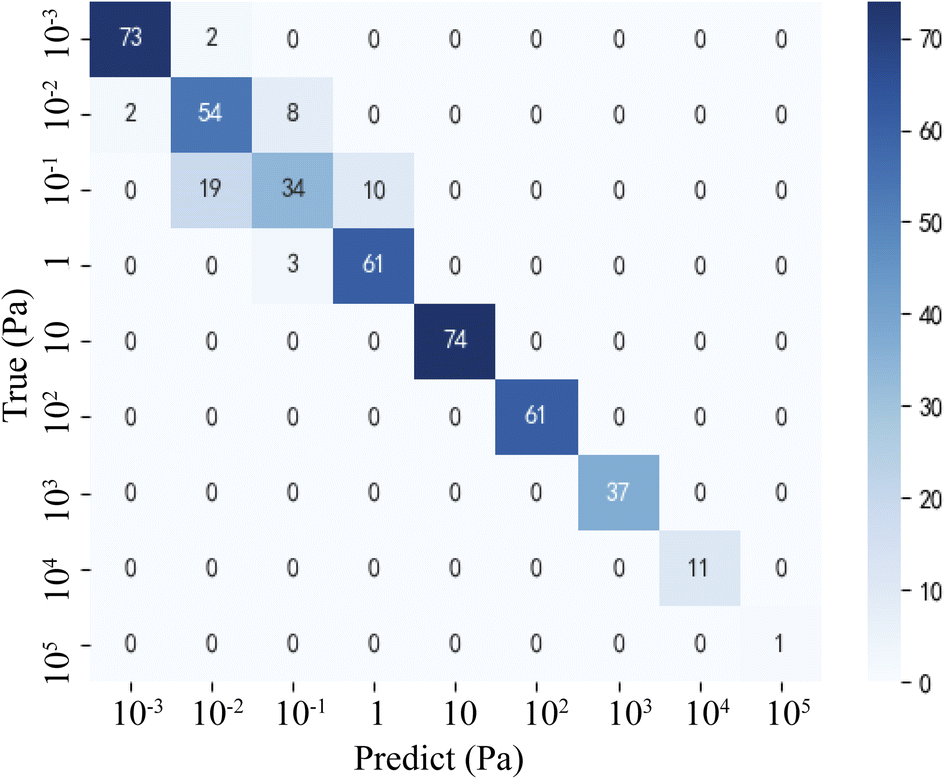 | ||
| Fig. 5 The visual representation of the confusion matrix for the RF vacuum level classification model. | ||
Furthermore, we performed calculations for accuracy, precision, recall, and F1 score to assess the overall performance of the classification model and its classification capabilities across different vacuum levels. The calculation methods are as follows:
 | (6) |
 | (7) |
 | (8) |
 | (9) |
In the context of vacuum level classification, a more specific illustration can be provided as follows: TP represents the accurate classification of samples with a vacuum level of 10−3 Pa into the category of 10−3 Pa. In this example, TN signifies the model's correct classification of samples that do not belong to the 10−3 Pa vacuum level into other vacuum level categories. This encompasses the samples that have been accurately classified under different vacuum levels. FP is indicative of the model incorrectly classifying samples that do not belong to the 10−3 Pa category as 10−3 Pa. This implies that the model has erroneously categorized samples from other vacuum levels as 10−3 Pa. FN, in contrast, refers to samples that originally belong to the 10−3 Pa category but have been mistakenly classified under different vacuum levels by the model. These cases represent instances where the model failed to detect low vacuum level samples accurately. The table below displays the computed results for different vacuum level categories, encompassing accuracy, precision, recall, and F1 score. These metrics are employed to assess the model's classification performance, reflecting both its overall capability and its ability to classify samples from different vacuum level categories accurately.
When assessing the vacuum level classification model, accuracy is employed to evaluate the model's overall classification capability. Precision indicates the model's performance in evaluating specific vacuum level categories. Recall signifies the model's ability to capture most of the true instances of a particular pressure level and avoid omissions. The F1 score represents the balance between accuracy and recall performance (Table 1). The table reveals that the model achieves an accuracy of 0.9145 or higher, indicating its strong classification performance. However, in lower vacuum level categories such as 10−2 Pa and 10−1 Pa, precision is relatively lower. The model excels in the 10−3 Pa category with minimal misclassifications, while it still performs well in the 10−2 Pa category but exhibits some false positives. In the 10−1 Pa category, the model demonstrates good classification performance but with a higher false negative rate, suggesting a need for improvement.
| Vacuum level categories (Pa) | Accuracy | Precision | Recall | F1 score |
|---|---|---|---|---|
| 10−3 | 0.9912 | 0.9733 | 0.9733 | 0.9733 |
| 10−2 | 0.9320 | 0.7200 | 0.8438 | 0.7770 |
| 10−1 | 0.9145 | 0.7727 | 0.5397 | 0.6355 |
| 1 | 0.9715 | 0.8472 | 0.9683 | 0.9037 |
| 10 | 0.9912 | 0.9610 | 0.9867 | 0.9737 |
| 102 | 0.9868 | 0.9531 | 0.9531 | 0.9531 |
| 103 | 0.9934 | 1.0000 | 0.0060 | 0.9610 |
| 104 | 1.0000 | 1.0000 | 1.0000 | 1.0000 |
| 105 | 1.0000 | 1.0000 | 1.0000 | 1.0000 |
4.3 Selection and optimization of spectral pretreatment methods
In this section, the application characteristics of distinguishing various vacuum level classes through spectra are utilized to fine-tune each preprocessing method to operate at its optimal state.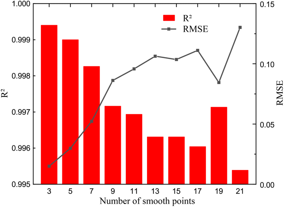 | ||
| Fig. 6 Selecting the best number of smoothing points for the 1st derivative method based on R2 and RMSE. | ||
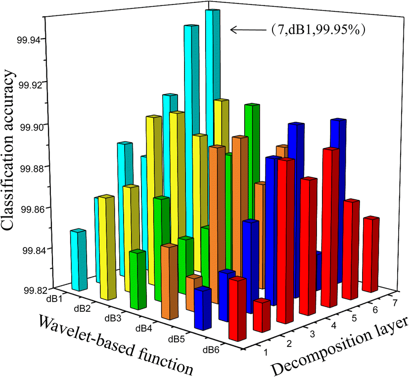 | ||
| Fig. 7 Optimal selection of wavelet-based function and decomposition layers based on classification accuracy. | ||
4.4 Random forest algorithm based on variable importance selection
Through the collection and initial analysis of the raw spectra, we observed a nearly monotonic trend in the integrated intensity of characteristic spectral lines for different elements with respect to pressure. This trend allowed us to conclude that using spectral intensity as raw data, we can classify the pressure level of the environment during spectral excitation using the random forest algorithm.However, in practice, using the integrated spectral line intensities as feature variables resulted in an accuracy rate of less than 80% due to the limited number of features. As a result, in subsequent experiments, all 1024 data points for each spectral line (a total of 4096 data points for the four elements) were used as raw data input. This decision led to an increase in accuracy at the expense of longer code execution time. To address this, the VIRF algorithm was introduced to filter out less informative data in the spectra, enhancing the model's reliability and reducing computational burden. Moreover, through experimentation, a suitable importance threshold was established to ensure that the feature set obtained during the filtering process accurately captures and describes the information within the spectral data. To be more specific, the performance of the original spectra in different vacuum degree environments reveals that certain input variables are informative, while others are non-informative. The difference in the performance of informative variables, such as CuI 515.3 nm, under different vacuum degree labels enhances the accuracy of the classification model. However, non-informative variables can increase the computational burden of the algorithm and reduce classification accuracy.
More importantly, to enhance the spectral distinctiveness within the same vacuum level and prevent overfitting of the RF model, variable importance in RF is employed as a feature selection technique to filter out the most discriminative and significant features from the original spectra. This further ensures the uniqueness of the feature set utilized in the classification task and underscores the crucial spectral attributes across different vacuum levels.
In this regard, we calculated the importance of the number of features by analyzing the difference between the OOB error when using a specific feature as the splitting condition and the average case. We plotted the importance of the variables of 4096 features when using original spectral lines as input, as shown in the figure below. Notably, we found that certain variables at specific wavelengths have zero importance values, indicating that they do not contribute to the vacuum classification algorithm. This not only increases the algorithm's running time but also adversely affects the vacuum classification performance of the model. Consequently, it is necessary to eliminate these uninformative variables through feature extraction and input variable optimization to enhance the algorithm's performance while preserving the integrity of the spectral information.
Based on Fig. 8, it can be observed that the majority of feature quantities have a significance level below 0.01. Therefore, we have chosen to set the importance threshold between 0 and 0.01 with increments of 0.001. This approach allows us to build multiple algorithm models with varying feature subsets, each with its own degree of importance.
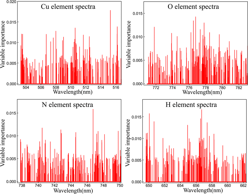 | ||
| Fig. 8 Variable importance information of raw spectra for four elements at each wavelength. | ||
The model was trained at various importance threshold values, and information such as the number of variables, R2, RMSE, OOB error, runtime, and accuracy are tabulated in Table 2 for horizontal comparison, aiming to select the optimal importance threshold. The first row of Table 2 represents the original random forest algorithm without threshold selection. A comparison reveals that the forest algorithm with threshold selection shows lower RMSE and OOB errors, while improving R2 and accuracy. This approach also significantly reduces the runtime by nearly 30%. From the table, it is evident that when the threshold is set to 0.009, all evaluation metrics are optimal. Thus, 0.009 is chosen as the threshold for variable importance in constructing the algorithm model.
| Thresholds | Number of variables | R 2 | RMSE | OOB error | Running time (s) | Accuracy rates (%) |
|---|---|---|---|---|---|---|
| M | 4096 | 0.9993 | 0.0151 | 0.32193 | 15.207 | 99.84 |
| 0 | 83 | 0.9996 | 0.0112 | 0.23471 | 11.362 | 99.90 |
| 0.001 | 82 | 0.9998 | 0.0069 | 0.21624 | 11.302 | 99.90 |
| 0.002 | 80 | 0.9995 | 0.0121 | 0.21618 | 11.189 | 99.85 |
| 0.003 | 79 | 0.9997 | 0.0094 | 0.25304 | 11.062 | 99.88 |
| 0.004 | 75 | 0.9996 | 0.0137 | 0.26900 | 11.046 | 99.81 |
| 0.005 | 73 | 0.9998 | 0.0060 | 0.20029 | 11.129 | 99.93 |
| 0.006 | 72 | 0.9998 | 0.00522 | 0.209333 | 11.026 | 99.942 |
| 0.007 | 70 | 0.9998 | 0.00737 | 0.225400 | 11.273 | 99.904 |
| 0.008 | 68 | 0.9997 | 0.00811 | 0.21589 | 11.230 | 99.898 |
| 0.009 | 61 | 0.9998 | 0.00507 | 0.18933 | 11.071 | 99.938 |
| 0.010 | 58 | 0.9999 | 0.00507 | 0.18607 | 11.125 | 99.929 |
In Fig. 9, it can be observed that all spectral pretreatment methods achieve satisfactory correlation coefficients, with multiple scattering correction showing relatively inferior performance as compared to the original spectral line, exhibiting lower R2 and higher RMSE values. The spectra processed with SNV demonstrated poorer performance in all four metrics compared to the original spectra. We speculate that this processing might have led to the loss of crucial peak information, resulting in a decrease in classification capability. Among the four methods, WT and VIRF exhibit similar performance in terms of R2, RMSE, and accuracy, with WT showing slightly lower OOB error. However, a closer examination in Table 2 reveals that VI-RF offers a significant advantage in terms of runtime compared to the raw data. When applying WT to the original data, it involves the selection of the most suitable parameters from various combinations of wavelet basis functions and decomposition layers to achieve the results shown in Fig. 9. This implies that WT requires a longer processing time compared to VI-RF. In complex field operating environments, VIRF offers a more straightforward and faster processing approach. Therefore, we believe VIRF is the most suitable algorithm for vacuum switch vacuum level classification.
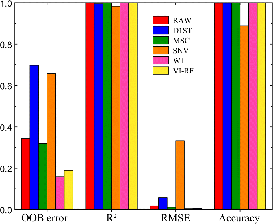 | ||
| Fig. 9 Performance comparison of different pretreatment methods. | ||
4.5 Optimization of model parameters
After optimizing the input spectrum for the model, it is essential to fine-tune the internal parameters of the model to ensure optimal performance in the vacuum degree classification scenario. The two most critical parameters in the model building step are the ntree within the forest and the mtry used for feature selection. The number of decision trees impacts whether voting can cover all input types, as too small a value for ntree can result in a loss of randomness, while too large a value can adversely affect the algorithm's efficiency or lead to overfitting.The classification effectiveness (i.e., accuracy) of the RF model depends on two factors: the smaller the correlation between any two trees in the forest, the higher the accuracy; and the stronger the classification ability of each tree in the forest, the higher the accuracy of the entire forest. Decreasing the number of mtry reduces the correlation and classification ability of trees in tandem, and vice versa. Thus, selecting appropriate values for these two parameters is crucial for achieving optimal accuracy and efficiency in the RF vacuum degree classification model.
To optimize the performance of the RF model, adjustments are made to ntree and mtry parameters. The ntree is varied from 0 to 100, while mtry ranges from M to M/20, where M represents the number of features in the original spectral data (4096). OOB error serves as the evaluation metric. The results presented in Fig. 10 indicate that when mtry exceeds M/4 (1024), the overall OOB error remains relatively high and increases with the increment of ntree. However, when mtry is less than M/4, the OOB error decreases with the reduction in mtry. The trend of OOB error with respect to changes in ntree aligns with the analysis in the previous chapter. Upon careful evaluation, we find that setting ntree to 50 and mtry to M/10 (410) results in the minimum OOB error, striking the optimal balance between computational efficiency and classification accuracy.
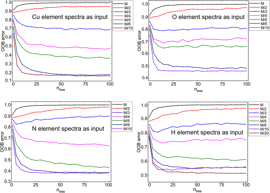 | ||
| Fig. 10 Determining the optimal ntree and mtry for the RF vacuum classification model using OOB error as the evaluation metric. | ||
4.6 Establishment and verification of RF in different vacuum degrees
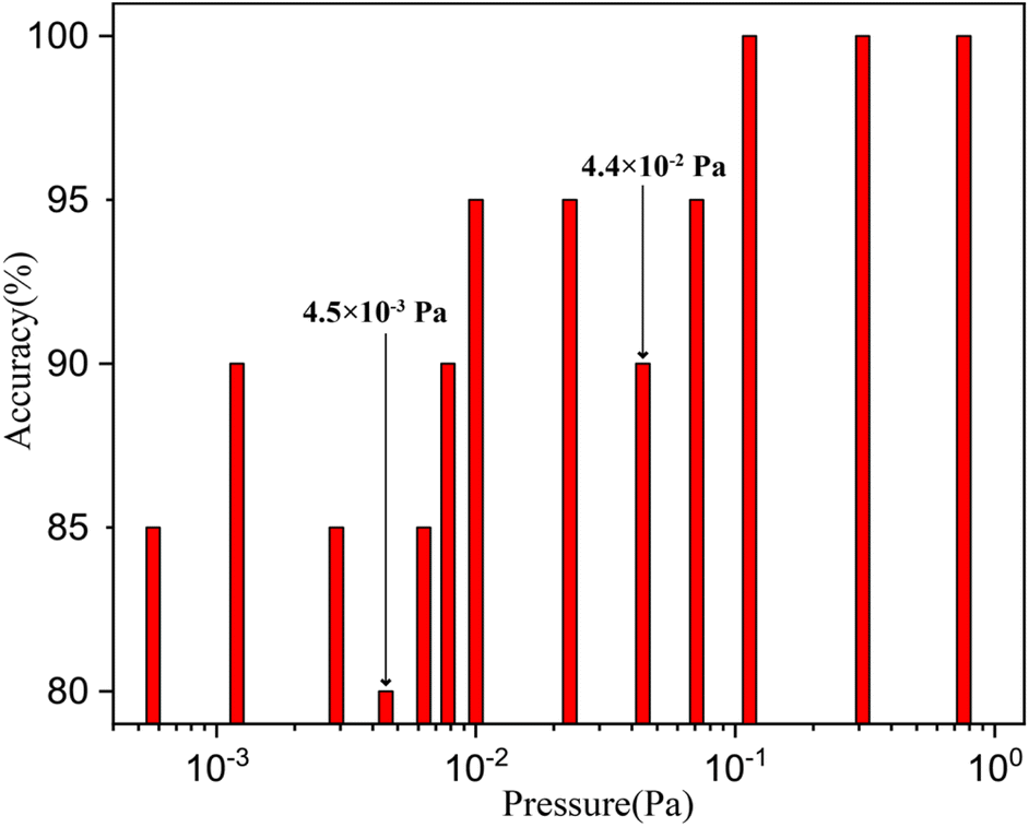
Under identical experimental conditions, additional experiments were conducted to evaluate the performance. In contrast to previous experiments, we randomly selected 30 vacuum levels within the range of 10−4 Pa to 105 Pa in our vacuum test platform. These levels include values such as 5.7 × 10⁻⁴ Pa, 1.2 × 10⁻³ Pa, 4.5 × 10⁻³ Pa, 7.8 × 10⁻³ Pa, 2.3 × 10⁻² Pa, and so on. The process for these 30 vacuum level settings involves reducing the chamber pressure to its minimum, followed by opening the pressure relief valve to simulate the leakage process in a real vacuum circuit breaker chamber. This experiment is employed to assess the classification model's accuracy in categorizing vacuum levels more precisely. This experiment aims to assess the accuracy of the classification model in categorizing more precise vacuum levels.Each vacuum level was measured 20 times, and the VIRF model was employed to calculate the accuracy for each tested vacuum level, as depicted in Fig. 11. Notably, the accuracy for vacuum levels above 10−1 Pa was omitted in the graph since it consistently approached 100%. This omission was made to provide a clearer analysis of differences in accuracy for low press.
 | ||
| Fig. 11 Validation of RF vacuum classification model accuracy at different pressure levels: an independent set of experiments. | ||
The result in Fig. 11 reveals the following findings: (1) As the air pressure decreases, the accuracy of classification decreases. However, once the pressure exceeds 10−1 Pa, the accuracy of vacuum degree classification reaches 100%. Combining spectroscopic analysis suggests that in high vacuum environments, where gas density is low, the differences in excitation of laser-induced plasma are not prominent, resulting in insufficient distinguishing features among different vacuum degree levels and consequently weaker classification capability. (2) Near the boundary between two different vacuum levels, there is a higher likelihood of classification errors, indicated by larger standard deviations in the classification results. For instance, when the vacuum level being tested is 4.5 × 10⁻³ Pa, and it gets classified as 10−3 Pa, we consider it correctly classified. However, in this scenario, the accuracy of vacuum level classification is only 80%, with 20% of measurements mistakenly classified as 10−2 Pa. The reason for this discrepancy lies in the fact that 4.5 × 10⁻³ Pa falls precisely at the boundary between the vacuum level of 10−3 Pa and 10−2 Pa. In an ideal situation, if the actual vacuum level is less than 5 × 10⁻³ Pa, classifying it as 10−3 Pa would be considered accurate. Similarly, if the actual vacuum level falls between 5 × 10⁻³ Pa and 5 × 10⁻² Pa, classifying it as 10−2 Pa would be considered correct, and so on.
Furthermore, the deeper reason for this phenomenon can be attributed to the idealized nature of the experiments in Fig. 9. To simplify the sampling process, we collected samples only for vacuum levels that were powers of 10 (these 9 same levels were used as classification labels for model training). In reality, there are theoretically numerous vacuum levels ranging from 10−3 Pa to 105 Pa., rather than making discrete jumps from 10−3 Pa to 10−2 Pa and subsequently to 10−1 Pa. Test pressures situated at the boundaries between two vacuum level categories exhibit relatively lower accuracy. This is due to the random forest algorithm model, which was originally developed for 9 discrete vacuum level categories as classification result labels. Using it to classify more precise, continuous vacuum levels results in reduced accuracy, representing a limitation of this model.
The overall results from the 30 experiments indicate that VI-RF achieved an accuracy of 96.7% within the range of 10−3 Pa to 105 Pa. Compared to other charge measurement methods, it offers lower detection limits and higher accuracy. Even with discrete classification results, it still assists engineers in assessing the risk of vacuum circuit breaker leakage, guiding maintenance operations, and identifying potential issues related to vacuum integrity.
5. Conclusions
In this study, we have introduced an innovative approach that combines LIBS technology with the VIRF algorithm for the online monitoring of vacuum levels in vacuum circuit breakers. This method is better suited for practical engineering applications, offering lower detection limits, higher precision, and user-friendly operation, with significant potential for widespread adoption.In order to simulate the actual structure of vacuum circuit breakers, we set up a LIBS-based vacuum level detection platform. We collected a total of 180 sets of original spectra for four elements (including Cu from the target material, and N, H, and O from the ambient gases) under different vacuum levels ranging from 10−3 to 105 Pa (10−3 Pa, 10−2 Pa,…, 104 Pa, 105 Pa). By comparing the changes in spectral features such as spectral broadening, peak heights, and integrated intensities of these elements with varying vacuum levels, we conceived the idea of characterizing vacuum levels using spectral information. We proposed a method that utilizes the Random Forest algorithm to classify vacuum levels based on spectral data. The original spectral data were divided into a training set and a test set in a 7:3 ratio, and we employed repeated k-fold cross-validation to increase the randomness of sampling validation, thereby enhancing the robustness of the classification process.
We assessed the overall accuracy of the algorithm and its classification precision for each vacuum level using visualized confusion matrices. To enhance the performance of the RF algorithm in the context of vacuum level detection based on spectral signals, we employed four preprocessing methods and compared their effectiveness in enhancing the distinctiveness of spectral data. This helped to prevent algorithm overfitting and improved stability. Subsequently, we employed VIRF for feature selection, eliminating redundant information and enhancing both the accuracy and operational speed of the algorithm.
Furthermore, during the model-building process, we optimized two critical parameters, ntree and mtry, using the OOB error as an evaluation metric. The R2 value for the algorithm's model is 0.9998, with an RMSE of 0.0051 and an accuracy of 98.94%. Lastly, under identical testing conditions, the algorithm was applied to 30 sets of vacuum data, covering a more finely graded range from 10−4 Pa to 105 Pa. The overall accuracy remained at 96.7%.
This algorithm currently has two limitations: (1) data limitations, as the algorithm can only categorize pressure measurements accurately to powers of ten (10−3 Pa, 10−2 Pa,…, 104 Pa, 105 Pa). It is hoped that future research can achieve a more precise classification scale. (2) Methodological limitations: at pressures of 10−1 and lower, there is still room for improvement in the algorithm's accuracy. This is due to the weaker spectral intensity, resulting in poorer differentiation. We hope that in future research, we can collect spectra with higher intensity and greater differentiation from the perspective of experimental design, such as through techniques like dual-pulse enhancement or nanoparticle-enhanced methods.
In conclusion, the method presented in this study provides a viable approach for online monitoring of vacuum levels in vacuum circuit breakers. It holds strong relevance to practical engineering applications, contributing to improved electrical grid operation safety and reliability. Additionally, it offers valuable insights for vacuum level measurements in other industrial sectors.
Conflicts of interest
There are no conflicts to declare.Acknowledgements
This work was supported by the National Natural Science Foundation of China (NSFC) (51777154, 51521065).References
- H. J. Dong, L. T. Ma, J. Li, X. Y. Guo and F. Z. Guo, High Volt. Technol., 2020, 46, 2539–2544 Search PubMed.
- S. W. Shu, J. J. Ruan, D. C. Huang, X. S. Chen, G. B. Wu and H. Li, High Volt. Technol., 2012, 38, 999–1005 Search PubMed.
- J. M. Wang, Power Equip., 2005, 1–5 Search PubMed.
- China Electric Power Research Institute, 12 kV–40.5 kV High Voltage Vacuum Circuit Breaker Ordering Technical Conditions, 2000, DL/T 403-2000, pp. 6–8 Search PubMed.
- Electric Power Research Institute of Ministry of Electric Power Industry, Wuhan High Voltage Research Institute of Ministry of Electric Power Industry and Xi’an Thermal Engineering Research Institute of Ministry of Electric Power Industry, Preventive Test Procedures for Power Equipment, 1996, DL/T 596-1996, pp. 34–36 Search PubMed.
- W. G. Li, T. Tian and J. Wu, Chin. J. Electr. Eng., 2008, 122–126 Search PubMed.
- W. G. Li, J. Wu and T. Tian, High Volt. Technol., 2007, 133–136 Search PubMed.
- M. Kamarol, S. Ohtsuka, M. Hikita, H. Saitou and M. Sakaki, IEEE Trans. Dielectr. Electr. Insul., 2007, 14, 593–599 Search PubMed.
- D. A. Cremers and L. J. Radziemski, Handbook of Laser-Induced Breakdown Spectroscopy. John Wiley & Sons, 2013 Search PubMed.
- F. J. Fortes, J. Moros, P. Lucena, L. M. Cabalin and J. J. Laserna, Anal. Chem., 2013, 85, 640–669 CrossRef CAS PubMed.
- M. A. Gondal, T. Hussain and Z. H. Yamani, Energy Sources, Part A, 2008, 30, 441–451 CrossRef CAS.
- M. Casini, M. A. Harith, V. Palleschi, A. Salvetti, D. P. Singh and M. Vaselli, Laser Part. Beams, 1991, 9, 633–639 CrossRef CAS.
- B. Connors, A. Somers and D. Day, Appl. Spectrosc., 2016, 70, 810–815 CrossRef.
- R. A. Multari, D. A. Cremers and M. L. Bostian, Appl. Opt., 2012, 51, B57–B64 CrossRef.
- X. Y. Liu and W. J. Zhang, J. Biomed. Sci. Eng., 2008, 1, 147 CrossRef.
- H. Tang, T. Zhang, X. Yang and H. Li, Anal. Methods, 2015, 7, 9171–9176 RSC.
- Q. J. Guo, H. B. Yu, Y. Xin, X. L. Li and X. H. Li, Spectrosc. Spectral Anal., 2010, 30, 783–787 Search PubMed.
- A. K. Rai, F. Y. Yueh and J. P. Singh, Appl. Opt., 2003, 42, 2078–2084 CrossRef.
- F. C. De Lucia and J. L. Gottfried, J. Phys. Chem. A, 2013, 117, 9555–9563 CrossRef.
- W. Rapin, P. Y. Meslin, S. Maurice, D. Vaniman, M. Nachon, N. Mangold, S. Schröder, O. Gasnault, O. Forni, R. C. Wiens, G. M. Martínez, A. Cousin, V. Sautter, J. Lasue, E. B. Rampe and D. Archer, Earth Planet. Sci. Lett., 2016, 452, 197–205 CrossRef.
- F. Rivera-Hernández, D. Y. Sumner, N. Mangold, K. M. Stack, O. Forni, H. Newsom, A. Williams, M. Nachon, J. l'Haridon and O. Gasnault, Icarus, 2019, 321, 82–98 CrossRef.
- O. A. Nassef, H. E. Ahmed and M. A. Harith, Anal. Methods, 2016, 8, 7096–7106 RSC.
- X. H. Wang, H. Yuan, D. X. Liu, P. Liu, L. Gao, H. B. Ding, W. T. Wang and M. Z. Rong, J. Phys. D: Appl. Phys., 2016, 49, 44LT01 CrossRef.
- H. Yuan, L. D. Song, P. Liu, X. H. Wang, D. X. Liu, A. J. Yang, H. B. Ding and M. Z. Rong, High Voltage Appliances, 2017, 53, 230–234 Search PubMed.
- H. Yuan, I. B. Gornushkin, A. B. Gojani, X. H. Wang and M. Z. Rong, Opt. Express, 2018, 26, 15962 CrossRef.
- H. Yuan, W. Ke, X. H. Wang, A. J. Yang, D. X. Liu and M. Z. Rong, High Volt. Technol., 2022, 48, 1160–1167 Search PubMed.
- M. Vahid Dastjerdi, S. J. Mousavi, M. Soltanolkotabi and A. Nezarati Zadeh, Iran. J. Sci. Technol., Trans. A: Sci., 2018, 42, 959–965 CrossRef.
- P. Yaroshchyk, D. Death and S. Spencer, J. Anal. At. Spectrom., 2012, 27, 92–98 RSC.
- L. Breiman, Mach. Learn., 2001, 45, 5–32 CrossRef.
- Z. Liuyang, M. Xiaohong, F. Weiqi, W. Rui, L. Zesheng, S. Yang and Z. Huafeng, Plasma Sci. Technol., 2019, 21, 034018 CrossRef.
- W. Yang, L. Mao-Gang, F. Ting, T.-L. Zhang, F. Ya-Qiang and L. Hua, Chin. J. Anal. Chem., 2022, 50, 100057 Search PubMed.
- T. Feng, X. Zhang, M. Li, T. Chen, L. Jiao, Y. Xu, H. Tang, T. Zhang and H. Li, Anal. Methods, 2021, 13, 3424–3432 RSC.
- S. Adusumilli, D. Bhatt, H. Wang, P. Bhattacharya and V. Devabhaktuni, Expert Syst. Appl., 2013, 40, 4653–4659 CrossRef.
- NIST, Atomic Spectra Database, National Institute of Standards and Technology, 2009 Search PubMed.
- A. Kning, N. Scherbarth, D. Cremers and M. Ferris, Appl. Spectrosc., 2000, 54, 331–340 CrossRef.
- B. Sallé, J. Lacour, E. Vors, P. Fichet, S. Maurice, D. A. Cremers and R. C. Wiens, Spectrochim. Acta, Part B, 2004, 59, 1413–1422 CrossRef.
- J. B. Sirven, B. Salle, P. Mauchien, J. L. Lacour, S. Maurice and G. Manhes, J. Anal. At. Spectrom., 2007, 22, 1471–1480 RSC.
- S. S. Harilal, N. Farid, J. R. Freeman, P. K. Diwakar, N. L. LaHaye and A. Hassanein, Appl. Phys. A: Mater. Sci. Process., 2014, 117, 319 CrossRef.
- A. Bogaerts, Z. Y. Chen, R. Gijbels and A. Vertes, Spectrochim. Acta, Part B, 2003, 58, 1867–1893 CrossRef.
| This journal is © The Royal Society of Chemistry 2024 |