 Open Access Article
 This Open Access Article is licensed under a Creative Commons Attribution-Non Commercial 3.0 Unported Licence
Are SAXS and SANS suitable to extract information on the role of water for electric-double-layer formation at the carbon–aqueous-electrolyte interface?†
Malina
Seyffertitz
 a,
Sebastian
Stock
ad,
Max Valentin
Rauscher
a,
Christian
Prehal
b,
Sylvio
Haas
c,
Lionel
Porcar
d and
Oskar
Paris
*a
a,
Sebastian
Stock
ad,
Max Valentin
Rauscher
a,
Christian
Prehal
b,
Sylvio
Haas
c,
Lionel
Porcar
d and
Oskar
Paris
*a
aChair of Physics, Department Physics, Mechanics and Electrical Engineering, Montanuniversitaet Leoben, Franz Josef Straße 18, 8700 Leoben, Austria. E-mail: oskar.paris@uniloeben.ac.at
bDepartment of Information Technology and Electrical Engineering, ETH Zürich, Gloriastrasse 35, 8092 Zurich, Switzerland
cDeutsches Elektronen-Synchrotron DESY, Notkestraße 85, 22607 Hamburg, Germany
dInstitut Laue-Langevin ILL, 71 avenue des Martyrs, 38042 Grenoble, France
First published on 16th August 2023
Abstract
This study reports on the applicability of X-ray transmission (XRT), small- and wide-angle X-ray scattering (SAXS/WAXS) and small-angle neutron scattering (SANS) for investigating fundamental processes taking place in the working electrode of an electric double-layer capacitor with 1 M RbBr aqueous electrolyte at different applied potentials. XRT and incoherent neutron scattering are employed to determine global ion- and water-concentration changes and associated charge-balancing mechanisms. We showcase the suitability of SAXS and SANS, respectively, to get complementary information on local ion and solvent rearrangement in nanoconfinement, but also underscore the limitations of simple qualitative models, asking for more quantitative descriptions of water–water and ion–water interactions via detailed atomistic modelling approaches.
Introduction
Electric double-layer (EDL) formation is the underlying physical process for important applications such as electric double-layer capacitors (EDLCs) or supercapacitors for electrical energy storage at high power density, as well as water desalination and remediation via capacitive deionization (CDI). The EDL formation is governed by the ion electrosorption at the electrode–electrolyte interface in the confined geometry of electronically conductive nanoporous electrode materials. Organic solvents are often preferred in technical EDLC applications due to a higher electrochemical stability window. Yet, water as an electrolyte solvent offers high ion mobility, low cost, reversible redox activity and an overall environmental friendliness, which, together with applications in CDI, highlights the importance of pursuing electrosorption studies on aqueous systems. Experimental evidence for an increased charge storage capacity of EDLCs was reported for sub-nanometer pores, which are smaller than the hydrated ions.1–3 Consequently, severe distortion of the ion hydration shell and/or (partial) desolvation of the ions at an energy cost upon entering small-sized pores were reported for organic as well as for aqueous electrolytes.4,5 Atomistic modelling also suggests ion clogging and co-ion trapping may occur in such (sub-)nanometer-sized pores, particularly if the applied potential is varied too quickly, resulting in slowed and sluggish charging dynamics.6,7 For organic electrolytes, the influence of confinement and desolvation on diffusive properties and ion transport with applied charges was simulated.8 It was shown theoretically and experimentally for aqueous electrolytes that even without an applied potential, water molecules prioritize forming a hydration structure with solvated ions over hydrogen bonding with other water molecules in carbon nanotubes.9,10 Other simulation work showed the decrement of the water's dielectric constant with increasing ion concentration.11 Pure water in nanoconfinement has been shown to exhibit an anomalously low dielectric constant,12,13 as well as the formation of high-density water (HDW) and low-density water (LDW).14–16 All these findings regarding ion transport phenomena, (de)solvation, and local dielectric properties suggest that the water molecules might be more than mere spectators, but rather a protagonist playing an active role in electric double-layer formation in nanoconfinement.Current EDL models, however, are often limited to mean-field descriptions of the density and dielectric properties, without considering the whole complexity of the solvent water. Experimental studies using straightforward intuition and the predictive power of simple analytical models are scarce. This might be due to the inherent difficulty of in situ monitoring the potential-driven ion electrosorption and related changes in water structure in the nanoconfinement of porous electrodes, which features the intricate interplay and mutual influence of varying electrostatic-, confinement- and chemical-concentration-dependent effects. Small-angle scattering (SAS) of X-rays (SAXS) and neutrons (SANS) is a well-established technique for investigating complex nanostructured systems, particularly if the system consists of two homogeneous phases separated by a sharp interface.17 SAS has also shown applicability in analyzing multi-component systems, such as EDLCs.5,18,19
However, the scattering signal of such multi-phase systems comprises contributions from the nanoporous solid electrode material, the electrolyte solvent and (at least) two different types of ions with changing local and global concentrations, rendering data interpretation extremely challenging. One possible way of dealing with this complexity is detailed atomistic modeling of the charged electrode based on real-space pore models, which can subsequently be compared to the in situ SAXS data.5 Another way of dealing with this difficulty is to apply contrast variation strategies using, e.g., anomalous SAXS (ASAXS) close to the absorption edges of the different ions, thus allowing the contribution of the respective resonating ions to be highlighted.20 While SAXS is not very sensitive to water, due to its much lower electron density as compared to (heavy) ions, neutrons have the great advantage of being particularly sensitive to the hydrogen nucleus. Thus, the neutron scattering length density of water may be comparable to or even higher than that of the ions. Moreover, by replacing water (H2O) with heavy water (D2O), the coherent and incoherent scattering lengths are strongly affected. Hence, a contrast variation strategy, by employing both SAXS and SANS using water and heavy water as a solvent on otherwise the very same system, comprises a potentially helpful step to better understand the specific role of water for EDL formation.
Here, we present and discuss results from in situ SAXS, in situ wide-angle X-ray scattering (WAXS), and in situ SANS from an EDLC using a porous activated carbon electrode and a 1 M aqueous RbBr electrolyte. On the one hand, in situ SAXS/WAXS and (energy-dependent) X-ray transmission measurements provide experimental access to the charge-balancing mechanism, global ion-concentration changes, and local ion rearrangement during charging and discharging. On the other hand, in situ SANS, as a highly hydrogen-sensitive technique, enables an H2O/D2O contrast variation of the electrolyte solvent to elucidate the solvent behavior during charging and discharging. Given the system's complexity, we aim to develop a mere qualitative understanding of the processes and understand the strengths and weaknesses of the different approaches and possible benefits of combining them.
Experimental
Materials
The investigated electrolyte salt was RbBr, acquired from Sigma Aldrich (99.6% trace metal basis). Electrolytes were prepared by mixing the solvent H2O (Milli-Q lab-grade H2O) or D2O (high-purity D2O received from Institut Laue Langevin, ILL) with the respective amount of salt to create a 1 M solution.All electrodes were prepared using commercially available MSP-20 (Kansai Coke and Chemicals Co.) activated carbon (AC) powder and 10 wt% PTFE binder (60 wt% solution in water, Sigma-Aldrich) following the protocol described in ref. 18. The AC powder and the binder were mixed with ethanol, rolled into sheets of 200 ± 10 μm or 300 ± 10 μm thickness using a rolling press, and dried at room temperature. Gas sorption analysis of the electrodes (Quantachrome/Anton Paar AutoSorb iQ) using N2 at 77 K and a slit pore QSDFT equilibrium kernel revealed a specific surface area of 1873 m2 g−1 and specific pore volume of 0.79 cm3 g−1, featuring almost exclusively microporous characteristics with the majority of pores being smaller than 2 nm. The respective pore-size distributions can be seen in the ESI, Fig. S1.† Electrodes of appropriate dimensions (see the respective section on in situ small-angle scattering) for SAXS and SANS investigations were punched from the free-standing electrode sheets. To ensure the removal of residual moisture, all electrodes were placed in a vacuum tube furnace at 125 °C for at least 24 hours prior to the in situ measurements.
In situ SAXS/WAXS and in situ SANS
The applied potential sequence during in situ investigations was controlled using a Gamry REF 600 or a Gamry Interface 1010B Potentiostat/Galvanostat. Each cell was conditioned after assembly and before the start of the SAXS/SANS experiments using three standard cyclic voltammetry (CV) cycles between 0.6 V and −0.6 V at a scan rate of 10 mV s−1. After conditioning, each cell was twice subjected to the following chronoamperometry measurement sequence: 0 V, 0.6 V, 0 V, −0.6 V, 0 V, and held for an hour at each potential.SAXS experiments were conducted at the P62 SAXSMAT beamline at Petra III at DESY in Hamburg, Germany, using a customized in situ SAXS cell similar to that in ref. 5, 18 and 21–23. The electrode set-up for SAXS was a classical coin cell consisting of a circular working electrode (WE) with dimensions of ø 6 mm × 200 μm thickness, a glass fibre separator (ø 40 mm × 200 μm thickness, Whatman GF/A), and a counter electrode (CE) with dimensions of ø 22 mm × 300 μm thickness. To irradiate the WE only, a ø 3 mm and ø 1.5 mm hole was punched in the CE and the separator, respectively. Both electrodes were in direct contact with the titanium cell walls, which acted as current collectors. A ø 2 mm opening was drilled into the titanium walls and covered with an approximately 3 mm sized scotch tape patch to seal the cell but allow the X-ray beam to pass. No conductive metal-foil as an additional current collector was added over the scotch tape piece. With this set-up, a CE/WE oversize factor of ≈20 was achieved. Each cell was filled with 320 μl of 1 M RbBr aqueous electrolyte. The X-ray beam was focused to a size of 840 μm × 920 μm. During the first CA potential sequence, the transmission, small-angle X-ray scattering (SAXS), and wide-angle X-ray scattering (WAXS) were measured with an acquisition time of 1 s at photon energies of 12.7 keV and 14.4 keV, i.e. below and above the K-edge of Br (13.47 keV), but below the K-edge of Rb (15.20 keV). Only 4 measurements per energy were conducted at each potential step during the first cycle. During the second CA cycle, the transmission, SAXS and WAXS signals were obtained at a fixed photon energy of 12.7 keV using an acquisition time of 1 s every 60 s. This resulted in a high time resolution of 60 data sets for each potential step, but kept radiation damage low. The SAXS/WAXS detectors used were an Eiger2 X 9M and a customized Eiger2 X 4M-DESY detector, respectively.
SANS experiments were conducted at the D22 small-angle neutron diffractometer at Institut Laue-Langevin, ILL, in Grenoble, France. Due to the considerably larger neutron beam (ø 10 mm) compared to the beam in the X-ray experiment, the electrode set-up was adapted to a “ring electrode” set-up instead of the classical coin cell. The WE was circular with dimensions of ø 12 mm × 200 μm thickness, the glass fibre separator was again ø 40 mm × 200 μm thickness and the CE was a ring with an inner diameter of øi 14 mm and an outer diameter of øo 36 mm and a uniform thickness of 200 μm. With this design, a WE/CE oversize factor of 7.6 was achieved. The same in situ cell as for SAXS was used, but with no central hole drilled into the titanium current collector cell walls, as the (0.5 mm thick) titanium is essentially transparent to neutrons. Each cell was filled with 450 μl of electrolyte. A diagram of the cell and the electrode set-up can be seen in Fig. S2.† The neutron wavelength was 4.3 Å. A SANS signal was recorded during the last 30 minutes of each 60 minute-long potential step, which resulted in 1 data set for each potential step.
SAXS and SANS data were azimuthally integrated and subjected to standard transmission and background correction procedures at the respective beamline/instrument. 1D SAXS/SANS profiles were represented as scattered intensity in relative units versus the length of the scattering vector, q = 4π![[thin space (1/6-em)]](https://www.rsc.org/images/entities/char_2009.gif) sin(θ)/λ, with 2θ being the scattering angle and λ being the wavelength of the respective radiation. No absolute intensity calibration was performed.
sin(θ)/λ, with 2θ being the scattering angle and λ being the wavelength of the respective radiation. No absolute intensity calibration was performed.
Results
X-ray transmission and X-ray scattering
All in situ X-ray measurements were conducted for two successive cycles with stepwise changes of the potential in the following sequence: 0 V, 0.6 V, 0 V, −0.6 V, 0 V. The current was monitored with a potentiostat. During the first cycle, measurements were conducted every 900 s at an energy of 12.7 keV and at other energies, which are, however, not discussed here, except for the transmission signal at 14.4 keV. During the second cycle, single measurements were made every 60 s at an energy of 12.7 keV.The X-ray transmission as a function of time is shown in Fig. 1. A systematic change in the transmission with applied potential is obtained, showing a reproducible behaviour for the two cycles. Generally, the transmission decreases upon applying a positive or a negative potential. This suggests that the ion concentration overall increases within the working electrode when a potential is applied, given that the absorption coefficients of Rb and Br are similar and much higher than that of water. The number of data points is lower in the first cycle, so its time resolution is limited. The well-resolved transmission signal in the second cycle suggests that changes do not always follow the potential steps immediately, but may change gradually over the whole holding time of 1 hour for the individual steps. For example, at +0.6 V, the transmission first decreases quickly, then decreases further, but at a much slower rate. In contrast, the transmission drops immediately at negative potential and stays essentially constant until the next potential step. At 0 V there are also some systematic differences in the time evolution depending on whether zero is approached from positive or negative potential. The original transmission at 0 V is not fully recovered, as there seems to be a slight but systematic overall decrease of the transmission signal with time. Also shown in Fig. 1 is the transmission at higher energy (14.4 keV), which lies in between the absorption edges of Br and Rb. This means that the linear absorption coefficient of Rb is only marginally changed, while that of Br is strongly enhanced, as seen in Table 1. This is indicated in the inset in the bottom right of Fig. 1, showing the imaginary part of the atomic scattering factor f′′ for Rb and Br,24 which is proportional to the linear attenuation coefficient for X-rays. The change in the energy not only has a drastic effect on the absolute value of the transmission (as compared to 12.7 keV), but also impacts the transmission changes with applied potential. While for positive potential there is now an even stronger drop in the transmission, it shows hardly any change for negative potential. As the transmission signal is now much more strongly influenced by the Br concentration, we conclude that there is a big change in the Br concentration for positive potential. At the same time, there seems to be hardly any Br mobilized for negative potential.
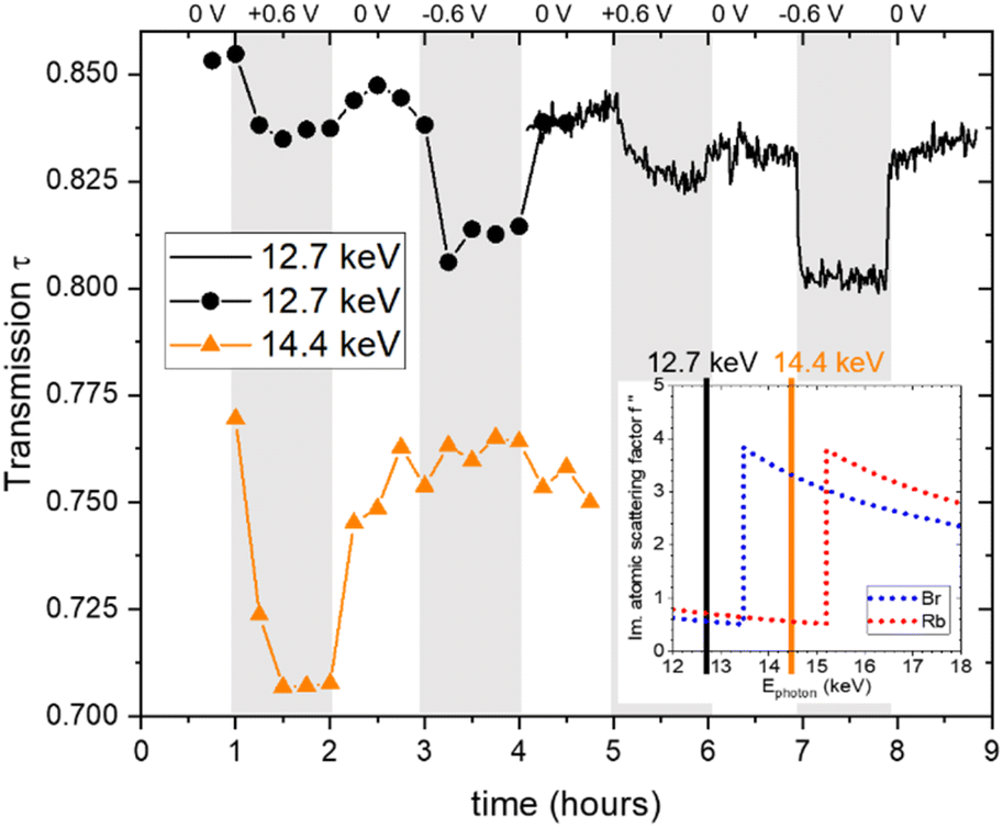 | ||
| Fig. 1 Measured X-ray transmission as a function of time, obtained at photon energies of 12.7 keV (black full line and black circles) and 14.4 keV (orange triangular symbols). The inset shows the progression of the imaginary part of the atomic scattering factor f′′ as a function of the X-ray energies for Rb and Br, with the inset data taken from ref. 24. | ||
| Rb+ | Br− | Carbon | H2O | D2O | ||||
|---|---|---|---|---|---|---|---|---|
| d bare | nm | 0.39 | 0.296 | |||||
| d hydr. | nm | 0.66 | 0.66 | |||||
| X-ray | μ(E) | 12.7 keV | cm−1 | 298.557 | 104.214 | 2.279 | 2.622 | |
| 14.4 keV | cm−1 | 206.762 | 526.09 | 1.545 | 1.81 | |||
| ρ el. | 1024 e− cm−3 | 2.65 | 1.164 | 0.572 | 0.334 | |||
| Neutron | σ | Absorption | cm−1 | 0.072 | 0.568 | 0.001 | 0.057 | 0.0 |
| Coherent | cm−1 | 0.464 | 0.186 | 0.529 | 0.004 | 0.513 | ||
| Incoherent | cm−1 | 0.037 | 0.003 | 0.0 | 5.621 | 0.138 | ||
| Attenuation | cm−1 | 0.573 | 0.758 | 0.53 | 5.682 | 0.651 | ||
| SLD | Coherent | 10−6 Å−2 | 5.214 | 2.186 | 6.001 | −0.561 | 6.393 | |
| Incoherent | 10−6 Å−2 | 1.47 | 0.296 | 0.0 | 21.18 | 3.321 | ||
Fig. 2 compares the SAXS (a) and the WAXS (b) scattering curves at 12.7 keV for the different steps, each curve representing the average over a full potential step for the second cycle. In Fig. 2c and d, all the single SAXS and WAXS curves were normalized to the average signal over the whole cycle for each q-value, and are shown in a heat-plot, red meaning an intensity increase and green an intensity decrease as compared to the average. This representation is very useful to highlight (q-dependent) changes in the scattering signal. The changes in both the SAXS and the WAXS intensities are different for negative and positive potential steps, while there are no major changes (neither with q nor with time) for the 0 V states being close to the average. We observe for the WAXS data in Fig. 2d quite considerable (time- and q-dependent) intensity changes at +0.6 V with a maximum around 35–40 nm−1. For −0.6 V, there is a sudden intensity increase with the potential step, with essentially no further time dependence (in agreement with the transmission), and only a moderate q-dependence. There seems to be an opposite change around 35–40 nm−1, i.e. a clear intensity increase at positive potential and an intensity drop (as compared to lower and higher q-values) for negative potential. Looking at the original scattering curves in Fig. 2b, this intensity change can be related to a shift in the correlation peak towards smaller q for positive potential and towards higher q for negative potential. We note that the integrated WAXS signal is proportional to the overall electron density in the beam and should therefore be related to global ion-concentration changes, similar to the in situ transmission data. Indeed, a comparison of the q-integrated WAXS signal and the negative logarithm of the transmission shows close similarity. This suggests that the ion transport at positive potential may occur slower or more sluggishly as compared to that at negative potential.
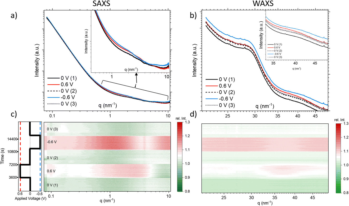 | ||
| Fig. 2 SAXS (a) and WAXS (b) scattering curves representing the average scattering at each applied potential step and corresponding heat-plots showing the scattering intensity relative to the average of all measurements for SAXS (c) and WAXS (d). | ||
The SAXS signal (Fig. 2c) also shows noticeable q-dependent intensity changes. The most obvious feature is a pronounced intensity enhancement centred around 2 nm−1 for positive potential, and an even stronger enhancement centred around 1 nm−1 for negative potential. For the largest q-values in the SAXS data, we find that the intensity is slightly below the average for positive potential, while it is clearly above for negative potential. On comparison with Fig. 2a, we see that these features are related to changes in the shape of the scattering curves, indicating the local redistribution of the ions (and the water) within the pores. The changes visible at very low q-values will not be considered here. Concluding on the X-ray results, we see that (1) there are time-dependent changes at long time scales (up to 1 h) seen in XRT, WAXS, and to some extent also in the SAXS data for positive potential, while the processes seem to be much faster for negative potential, and (2) the intensity shows strongly q-dependent changes for positive potential, while there seems to be a much less q-dependent overall intensity increase for negative potential, similar to the minor changes of the 0 V states.
Fig. 3a displays the SANS curves at each potential step, with the electrolyte solvent water (H2O) represented in light blue and heavy water (D2O) in dark blue. Unlike the SAXS data, where multiple curves were measured for each potential step, only a single SANS curve was obtained for each potential step, excluding considerations about time dependence in SANS. From Fig. 3a, it is evident that the scattering curves when using H2O exhibit a generally higher intensity compared to those obtained with D2O. The scattering curves recorded at different potentials display a high degree of concurrence, suggesting only minimal potential-dependent changes. The insets in Fig. 3a present a zoomed-in view of the scattering signals within the q-range of 9.0–9.7 nm−1, for the sake of clarity only for the first CA cycle. These reveal very subtle yet systematic changes in intensity. Fig. 3b presents the average of these scattering intensities in the q-range of 9.0–9.7 nm−1 for H2O (depicted by light-blue rectangles) and heavy water (D2O, represented by dark-blue triangles) for both cycles at each applied potential. Due to the very large incoherent scattering cross-section of hydrogen, we expect the intensity in this q-range to be directly proportional to the water concentration for H2O. For D2O, the coherent and incoherent scattering cross-sections are similar (see Table 1).
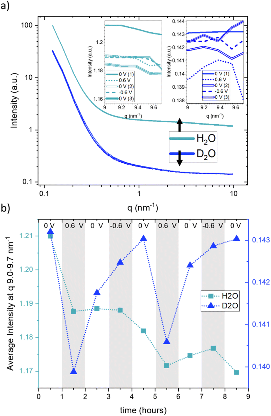 | ||
| Fig. 3 SANS curves (a) and average SANS intensity in the q-range from 9.0–9.7 nm−1 (b) for H2O (light-blue rectangles) and D2O (dark-blue triangles). The insets in (a) show the scattering intensity in the q-range of 9.0–9.7 nm−1. | ||
Therefore, a stronger influence from coherent scattering, and thus, q-dependent intensity changes, may be present. A noticeable intensity decrease is observed for H2O in Fig. 3b for the first step from 0 V to 0.6 V, which is (although at a somewhat lower amount) also seen for the second step from 0 V to 0.6 V. In both cases, the intensity does not return to the original value when the potential is removed, which results in an overall decrease in the intensity. This can only be understood via an overall decrease in the amount of water in the working electrode. D2O exhibits more systematic potential-dependent changes, with a prominent minimum at positive potential. Yet, the original value at 0 V is also not recovered when going from +0.6 V to 0 V, but only after the change from −0.6 V to 0 V. This behavior is fully reproducible for the second cycle. This observation suggests a dependence of the equilibrium state on the preceding potential history, indicating that the behaviour of the system at zero applied potential is not the same following potential steps of 0.6 V and −0.6 V. Considering the SANS signal was collected in the latter half of each 60-minute potential step, we acknowledge that this averaging over long periods of time may also influence the observed different data at 0 V. The disparate behavior of the 0 V contribution could potentially also be due to kinetic effects, which are also seen for SAXS in Fig. 1, particularly for negative potentials. It is worth noting that the absolute value for the average intensity in this q-range is higher by a factor of 8.3 for H2O as compared to D2O. This corresponds well to the calculated value considering both the incoherent and coherent scattering length densities for H2O and D2O. ((SLDinc,H2O2 + SLDcoh,H2O2)/(SLDinc,D2O2 + SLDcoh,D2O2) = 8.65).
Since the absolute value of the incoherent scattering length density of H2O is larger by 37.7 compared to its coherent scattering length density (corresponding to a ratio of ≈1400 for the cross section), it is reasonable to assume that the signal at high q is exclusively governed by incoherent scattering from water. We have, therefore, subtracted this average value from the scattering data of H2O. D2O has also a substantial incoherent scattering contribution, yet the coherent scattering length density is larger than the incoherent one by roughly a factor of two and hence the coherent cross-section is larger by roughly a factor of four as compared to the incoherent cross-section. Therefore, we subtracted from the D2O data the value for H2O, scaled by the ratio of their incoherent scattering length densities: (SLDinc,D2O/SLDinc,H2O)2 = 1/40.68. The resulting scattering curves and corresponding heat plots, akin to the representation for X-rays, are illustrated in Fig. 4, with panels (a) and (c) representing H2O, and panels (b) and (d) representing D2O.
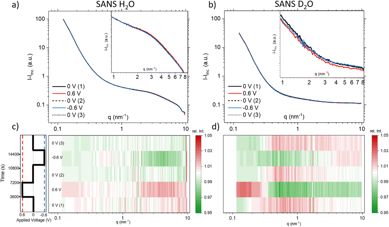 | ||
| Fig. 4 Coherent SANS scattering curves and corresponding heat-plots displaying relative intensity changes for H2O (a) and (c), and D2O (b) and (d). | ||
A pronounced hump in the coherent scattering signal can be seen for H2O (Fig. 4a) at around 4 nm−1, which is absent for D2O (Fig. 4b). This hump is associated with nanopores in the activated carbon electrode, which when filled with H2O show a pronounced SANS contrast, i.e. coherent scattering length density difference (Table 1), as compared to the almost perfect contrast matching of D2O-filled pores. More detailed depictions of SANS measurements of the “empty” carbon electrode, and when infiltrated with H2O and D2O, can be seen in the ESI, Fig. S3.† The coherent part of the SANS data shown in Fig. 4a and b demonstrates only small potential-dependent changes compared to SAXS and WAXS. The heat plots in Fig. 4c and d indicate relative changes of approximately ±5%, while the observed relative changes in SAXS (see Fig. 2) are in the order of ±25%. H2O (Fig. 4c) exhibits for q > 2 nm−1 an increase in the relative scattering intensity for positive applied potential, while a decrease is observed for negative applied potential as compared to the average. In contrast, for D2O (Fig. 4d), the opposite trend is observed for large q, with a minimum for positive applied potential and a maximum for negative applied potential. For smaller q around 1 nm−1, there seems to be an intensity decrease for both positive and negative potentials for D2O, while there is hardly any trend visible for H2O.
Discussion
Global ion- and water-concentration changes
Charge balancing in EDLCs can be categorized into three basic mechanisms: (1) the desorption of co-ions (co-ion expulsion), where the concentration of counter-ions remains constant, (2) the adsorption of counter-ions (counter-ion adsorption), where the concentration of co-ions remains constant and (3) ion exchange, which is a combination of (1) and (2) and thus, the total number of ions within the electrode remains unchanged.25Fig. 5a shows a schematic drawing of these charge-balancing mechanisms. The total electrosorbed charge can be calculated from the electrochemical signal via the integration of the measured current signal over time.18,23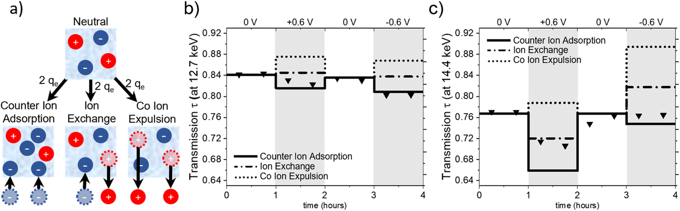 | ||
| Fig. 5 (a) Schematic representation of the charge-balancing mechanisms. Calculated transmission for counter-ion adsorption (full line), ion exchange (dash-dotted line) and co-ion expulsion (dotted line) as well as measured transmission (triangular symbols) for X-ray energies of (b) 12.7 keV and (c) 14.4 keV. | ||
To set up a simple model for assessing global ion- and water-concentration changes at the working electrode, we make the following assumptions: firstly, the pore volume of the activated carbon electrode remains constant, with negligible adsorption deformation.22 Secondly, the total volume fraction of electrolyte in the beam is represented by the sum of the volume fractions of anions (wan), cations (wcat) and water (ww), i.e. wan + wcat + ww = 1. Lastly, we do not consider density changes in the solvent within the carbon confinement or the ion hydration shell. The objective of this model is to evaluate its validity and assess whether any modifications are required based on our observations.
The X-ray transmission (XRT) signal follows the Beer–Lambert law (τ = e−μ(E)d), depending on the material-specific and photon-energy-dependent linear attenuation coefficient μ(E) and the penetrated sample thickness d. The negative logarithm of the transmission is, thus, directly related to the sum of the energy dependent linear attenuation coefficients μ(E) of water (w), cation (ca) and anion (an), weighted by their respective volume fractions w in the irradiated electrolyte thickness del:18,21
| −ln(τ(E)) = (ww × μw(E) + wcat × μcat(E) + wan × μan(E)) × del + μC(E) × dC | (1) |
Assuming an initial ion concentration of 1 M within the electrode and every single charge-bearing cation and anion contributing one elementary charge to the EDL, theoretical concentration changes of the ions at the working electrode can be calculated for the three charge-balancing mechanisms. In our previous studies,18,23 changes in the concentration of water in the irradiated sample volume were not considered since the absorption coefficient for water molecules is much lower as compared to that for the ions. Here, we explicitly compensate for the vacated or taken-up volume resulting from the movement of ions under the assumption of a constant irradiated volume of electrolyte within the beam by adjusting the corresponding amount of H2O at a 1 g cm−3 density. In this way, the calculated volume fractions of cations, anions, and water molecules allow the assessment of theoretical transmission values for a specific photon energy for each charge-balancing mechanism.
Fig. 5 illustrates the calculated transmission values for pure ion exchange (dash-dotted line), pure co-ion expulsion (dotted line), and pure counter-ion adsorption (solid line). The measured transmission values are represented as triangular symbols at (a) 12.7 keV (below the absorption edges of Rb and Br) and (b) 14.4 keV (above the Br but below the Rb edge).
From Fig. 5a, it seems evident that the transmission at 12.7 keV closely aligns with the calculated progression for counter-ion adsorption. However, this is less clear for the second energy of 14.4 keV (Fig. 5c), with the suggested mechanism lying closer to ion exchange for positive potential and closer to counter-ion (i.e. cation) adsorption for negative potential. At 14.4 keV, i.e. above the absorption edge of Br, the transmission signal is strongly influenced by changes in the Br concentration. The data suggests the charge-balancing to be primarily driven by ion exchange, with a subtle inclination towards counter ion adsorption at positive applied potential. At negative applied potential, the 14.4 keV transmission signal suggests an interplay between counter ion adsorption and ion exchange. Considering the substantially smaller absolute changes in transmission at 12.7 keV, we expect a higher uncertainty due to systematic errors, e.g., uncertainties in the ion volumes taken from the literature (Table 1) and possible influences of electrode swelling.22
In light of these findings, we would like to re-emphasize the distinct behaviour observed in the time-resolved transmission signal, as depicted in Fig. 1. We note here again the more gradual change in the transmission signal at positive applied potential to the almost instantaneous drop in the X-ray transmission at negative applied potential, which indicated a slower change in the Br− concentration compared to the local Rb+ concentration at the working electrode, even though Br− and Rb+ have been reported to exhibit similar ion mobility in bulk aqueous solutions.29
This finding aligns only qualitatively with our previous results on the same system with slightly different cell geometry,21 which demonstrated first a fast charge-balancing mechanism of ion exchange followed by a much slower (diffuse) equilibration transition towards counter-ion adsorption for positive potential and ion exchange for negative potential. Moreover, in another study using a different electrode material with 1 M RbBr electrolyte, we even found a tendency towards co-ion expulsion for positive potential and ion exchange for negative potential.20 This underlines that the overall charge-balancing mechanism may depend strongly on subtle details, which are experimentally difficult to control. The influence of electrode geometry and the volume of the electrolyte reservoir has already been discussed in ref. 21. In our specific experimental set-up, 320 μl of electrolyte was utilized, with an estimated volume of approximately 3.6 μl wetting the porous space of the working electrode. This results in an electrolyte-to-reservoir ratio of about 100, which according to ref. 21 should promote the transition from ion exchange to counter-ion adsorption. In addition to cell geometry and electrolyte-reservoir size, more subtle mechanisms such as ion clogging and co-ion trapping may lead to metastable states depending on the details of the potential sweep and the history of the previous states.6,7
In this context, we also emphasize the potential role of water. If the overall density of water varies with different applied potentials, it will necessitate replacing the simple model in eqn (1) with a density-dependent water contribution. This influence becomes plausible if the density of water depends on the confinement.15 Our SANS measurements with pure H2O in the electrode provide experimental evidence that the water density is non-uniform within the nanopores (see Fig. S3 in the ESI†). Moreover, if the anions and cations carry water hydration shells with different densities compared to the bulk, the global ion fluxes as well as the potential-dependent partial loss of the water shell in confinement30 would influence the measured X-ray transmission. Despite the literature reporting similar water mass density in the shells of Rb and Br,31 and the fact that X-rays are not very sensitive to water as compared to the ions, the discrepancies in the observed mechanisms in the present experiments at two X-ray energies hint towards a non-negligible influence of water.
One of the biggest advantages of SANS compared to SAXS in this respect is its high sensitivity for hydrogen and, thus, water. In particular, the incoherent cross-section of H2O is larger by more than three orders of magnitude as compared to its coherent cross-section (Table 1), and also the incoherent and coherent cross-sections of Rb and Br are negligible in this respect. This means that for high enough q-values, the SANS intensity given by  is independent of q and thus, the change in the SANS intensity is directly proportional to the change in water concentration in the beam. Fig. 3b suggests a strong decrease in the water concentration at a positive potential, which would go hand-in-hand with the increase in the total ion concentration in the electrode according to the counter-ion adsorption found from X-ray transmission. For negative potential, the XRT data suggest a trend towards ion exchange, which means that within our simple model the overall water concentration also should not change significantly, due to the comparable ion size. This is qualitatively in agreement with the almost-constant incoherent H2O intensity in Fig. 3b when changing the potential from 0 V to −0.6 V. We also note that there is an overall decrease in water concentration over the two measured cycles in Fig. 3b, which is qualitatively consistent with the slight overall decrease in the transmission signal in Fig. 1, suggesting an overall ion-concentration increase. However, when applying the simple model described in analogy to eqn (1) to the SANS data as presented in Fig. 3b, the observed changes are larger than what would be expected from the exchange of occupied ion volume by water at bulk density. This suggests that these simple considerations are not applicable to water in confinement at charged interfaces. We abstain from a more detailed quantitative comparison here, particularly because laboratory X-ray transmission data from the SANS cell do not fully coincide with those from the SAXS cell, suggesting non-negligible influences of the cell geometry on the global ion-exchange mechanism.
The SANS signal for D2O in Fig. 3b shows a different behaviour to that of H2O. This is not surprising since, for D2O, the incoherent scattering length density is considerably smaller than the coherent one. Also, the coherent scattering length densities of the ions are in the same order of magnitude and hence for large q values it should hold that:
 | (2) |
Even when assuming the coherent intensity reaches a constant value for large q, it will depend on the concentration changes in D2O and both ion species, and is complicated to interpret.
Local ion re-arrangement
While the X-ray transmission and the incoherent scattering from H2O are useful for estimating the charge-balancing mechanisms and global ion-concentration changes, they do not provide information on local ion rearrangement in confinement. To address the question of local ion rearrangement, in situ SAXS and coherent in situ SANS measurements provide q-dependent intensity changes, which are related to confinement-dependent re-organisation of cations, anions, and water molecules upon applying a positive or negative potential. Moreover, the WAXS signal is sensitive to local correlations between atoms and molecules, represented by their partial structure factors. Although the present system is too complex to be analysed quantitatively, characteristic changes in the overall structure factor may also be qualitatively interpreted. We first assume that the measured intensity can be written as the sum of three independent terms:| I(q) = IP(q) + INP(q) + ISF(q) | (3) |
The first term is related to the scattering at very small q, described by the power law IP(q) = A/qα from the scattering of the carbon powder grains surrounded by electrolyte. This term is difficult to interpret and will be skipped in the following. The second term, INP(q), is associated with the scattering signal in an intermediate q region and describes the small-angle scattering of the electrolyte within the carbon nanopores. For a simple two-phase system, INP(q) would be proportional to the scattering contrast K, i.e., the squared electron density difference between the constituting phases. However, the electrolyte within the pores cannot be simply treated as a homogeneous phase, since the re-arrangement of the ions and potentially also the confinement-dependent changing water density within the carbon nanopores lead to the observed q-dependent changes in the SAXS signal in the intermediate q-region around 1 nm−1. As the SAXS signal decreases strongly with increasing q, the contribution of the third term, i.e. the structure factor ISF(q), becomes more prominent, extending into the WAXS regime. The structure factor is often considered constant in the small-angle scattering regime, as the typical atomic/molecular correlation maxima of the electrolyte or carbon appear around 15–20 nm−1 (corresponding to typical atomic distances of 0.3–0.4 nm). Yet, we see in Fig. 2a an intensity increase in the SAXS data around 9–10 nm−1, suggesting a non-trivial (i.e. q-dependent) influence of the structure factor also in the SAXS regime. In other words, it is challenging to clearly define the crossover from SAXS (describing local ion and water redistribution within geometrically well-defined nanopores) to WAXS (describing atomic/molecular correlations between the different species in the form of partial structure factors). Yet, this q-range corresponds precisely to the size of single hydrated ions (around 0.7 nm) and, therefore, to the region where ion de-hydration starts to become important.1,5,32 In accordance with our previous work, we attribute the intensity changes in the range between ≈0.5 nm−1 and ≈5 nm−1 to INP(q), i.e., local ion re-arrangement within the pores, while the changes around 10 nm−1 and in the WAXS data are related to structure-factor changes, ISF(q).
The interpretation of relative SAXS intensity changes concerning ion rearrangement within nanopores presents challenges, as discussed in ref. 18. It is not possible to a priori distinguish between a local change in ion concentration within a pore of a specific size and the redistribution of ions within the pore, such as counter-ions moving towards the pore wall and co-ions moving away from the wall. To quantitatively correlate SAXS intensity changes with confinement-dependent ion re-arrangement, detailed atomistic modelling, as demonstrated in ref. 5, would be necessary, which is beyond the scope of this work. Here, we focus on discussing general trends that can aid in understanding the influence of water on local ion rearrangement.
The observed “maxima” in Fig. 2c are situated within the intermediate q-range associated with INP(q). Assuming a simple two-phase system, comprising carbon as one phase and the electrolyte as a homogeneous phase, would result in a changed SAXS contrast K = (ρC − ρel)2, which would cause a simple vertical shift of the SAXS scattering curve on a logarithmic scale. However, this increase is not directly and unequivocally linked to a specific pore size due to interference from structure-factor effects and local rearrangements. The distinct relative intensity maxima observed at approximately 2 nm−1 for positive applied potential (corresponding to increased Br− concentration) and 1 nm−1 for negative applied potential (corresponding to increased Rb+ concentration) point towards a more complex rearrangement scenario and indicate that the local re-arrangement of the two ion species, Rb+ and Br−, differs. The shift of the maxima towards higher q values for positive potentials indicates that Br− prefers higher confinement compared to Rb+, potentially leading to a higher degree of desolvation. This finding is surprising considering that Br+ and Rb+ are reported to have similar hydration enthalpies,29 and Br+ is also larger in a desolvated state.
When examining the D2O SANS signal, as illustrated in Fig. 4d, we observe a decrease in intensity for intermediate q-values around 1 nm−1 for both positive and negative potentials, with the relative intensity minimum again being shifted towards higher q values for positive potentials and towards smaller q values for negative potential. This change is consistent with the SAXS results. Only the direction of the SAXS intensity change is the opposite, due to the different contrasts. The same ion rearrangement described from SAXS can lead to an opposite relative SANS intensity when using D2O as a solvent (Table 1), as the coherent scattering length densities of D2O and the carbon matrix almost perfectly contrast-match.
Analysing the coherent H2O SANS data, as depicted in Fig. 4c in the intermediate q region, could offer insights into the local rearrangement of water molecules within nanopores. Given that H2O exhibits a significantly larger coherent scattering length density difference with respect to carbon in comparison to the ions, it should dominate the corresponding SANS signal. Interestingly, we observe a lack of significant variations in the intermediate q-range, indicating the absence of substantial rearrangement or reorganization of water molecules within the nanopores as the applied potential is varied.
We conclude that there is no drastic change in the local water distribution within the nanopores (from SANS using H2O), while there is a strong local ion re-arrangement (from SAXS and SANS using D2O), upon charging and discharging. Future atomistic modelling approaches similar to those in ref. 5 may provide more quantitative results.
Structure factor
At q-values around 10 nm−1, the relative SAXS data exhibit a minimum at positive potential and a maximum at negative potential (Fig. 2c). The opposite trend is observed in the WAXS data around 40 nm−1, with a maximum at positive potential and a slight minimum at negative potential. Furthermore, the relative SANS changes for D2O (Fig. 4d) display a qualitatively similar behaviour to the SAXS data in the high q-region. Upon closer examination of the WAXS curves in Fig. 2b, it becomes evident that the intensity increase observed around 40 nm−1 for positive potentials is accompanied by a peak shift towards smaller q-values. For negative potential, there is a slight, albeit less pronounced, peak shift towards larger q-values. A broad peak around 40 nm−1 was also reported for bulk aqueous RbBr solutions using X-ray and neutron diffraction,33 being fully absent in the structure factor of pure water.34 We believe that this peak is intimately connected to the hydration shells of the Rb and/or Br ions, as we find such a peak neither for the bare carbon electrode nor for the carbon electrode soaked with pure water. Therefore, we tentatively relate the potential-dependent shift of this peak to a different ion de-hydration scenario of Br− and Rb+ in strong confinement.Inspecting the associated H2O SANS data (Fig. 4c) close to 10 nm−1, a minimum at negative and a maximum at positive potential are observed, opposite to the behaviour for D2O SANS/SAXS. Since X-rays are practically insensitive to hydrogen, the changes in the SAXS and WAXS data may be due to oxygen–oxygen as well as oxygen–anion and oxygen–cation correlations. As SANS also includes all the partial structure factors related to the correlation with hydrogen (deuterium), a different structure-factor behaviour as observed in our data is not unexpected. We believe that the found changes in partial structure factors are mainly related to the ion hydration structure, which changes upon entering very small nanopores.1,4,5
More detailed statements about these phenomena would require knowledge about the interplay of associated partial structure factors, which results in at least 10 single distributions, even if the solvent is treated as a single, homogeneous phase. A straightforward quantitative analysis is not feasible without further modelling-based support.
Conclusions
In this study, we conducted in situ XRT measurements at different photon energies, as well as in situ SAXS/WAXS and in situ SANS using H2O and D2O to study ion electrosorption in a nanoporous carbon working electrode using a 1 M aqueous RbBr electrolyte. We have drawn the following conclusions:(1) XRT is a valuable technique for extracting information regarding global ion-concentration changes at the working electrode, and determining the mechanism of charge balancing. Analysing the incoherent contributions in SANS is useful to understand variations in the water concentration upon charging and discharging.
(2) When examining confinement-related phenomena, SAXS and SANS data in the intermediate q-regime provide insights into the rearrangement of ions and water molecules within the nanopores. Our results indicate a notable difference concerning the rearrangement of Rb+ cations and Br− anions upon charging. No significant rearrangement of water molecules within the nanoconfinement was observed.
(3) The inspection of SAXS/SANS signals at high q-values, as well as the WAXS signals, may contribute to understanding the behaviour of partial ion–solvent and solvent–solvent structure factors. Nonetheless, data interpretation in this context poses significant challenges.
(4) SAXS provides valuable information regarding ions, while SANS, being a hydrogen-sensitive technique, offers insights into solvent molecules.
Future experiment-based investigations could encompass different electrolyte salts with varying hydration enthalpies, extending SANS towards higher q-values and conducting SAXS measurements on the same electrode geometry/set-up as for the SANS measurements. Combined with a simulation- and modelling-based analysis, this could provide a more comprehensive and complete picture of the active role of water in electric double-layer formation.
Author contributions
M. S.: conceptualization, investigation, data curation, visualization, writing – original draft, writing – review & editing; S. S.: investigation, writing – review & editing; M. V. R.: investigation, writing – review & editing; C. P.: writing – review & editing; S. H.: investigation, data curation, writing – review & editing; L. P.: investigation, data curation, writing – review & editing; O. P.: conceptualization, writing – original draft, writing – review & editing, supervision.Data availability
The data associated with the ILL beamtime can be accessed at https://doi.org/10.5291/ILL-DATA.6-07-104.Conflicts of interest
There are no conflicts to declare.Acknowledgements
The authors would like to acknowledge the allocation of beamtime at the Deutsches Elektronen-Synchrotron (DESY) under proposal I-20220173 EC, as well as at the Institut Laue-Langevin (ILL) under proposals 01-04-228 and 6-07-104. We express our gratitude to both facilities for their support and assistance in conducting the measurements. The authors would also like to express their gratitude to Peter Moharitsch from the Chair of Physics at Montanuniversitaet Leoben for machining and support with the in situ SAXS and SANS cells.References
- C. Merlet, C. Péan, B. Rotenberg, P. A. Madden, B. Daffos, P. L. Taberna, P. Simon and M. Salanne, Nat. Commun., 2013, 4, 2701 CrossRef CAS.
- J. Chmiola, G. Yushin, Y. Gogotsi, C. Portet, P. Simon and P. L. Taberna, Science, 2006, 313, 1760–1763 CrossRef CAS.
- N. Ganfoud, A. Sene, M. Haefele, A. Marin-Laflèche, B. Daffos, P.-L. Taberna, M. Salanne, P. Simon and B. Rotenberg, Energy Storage Mater., 2019, 21, 190–195 CrossRef.
- J. Chmiola, C. Largeot, P. L. Taberna, P. Simon and Y. Gogotsi, Angew. Chem., Int. Ed., 2008, 47, 3392–3395 CrossRef CAS PubMed.
- C. Prehal, C. Koczwara, N. Jäckel, A. Schreiber, M. Burian, H. Amenitsch, M. A. Hartmann, V. Presser and O. Paris, Nat. Energy, 2017, 2, 16215 CrossRef CAS.
- K. Breitsprecher, C. Holm and S. Kondrat, ACS Nano, 2018, 12, 9733–9741 CrossRef CAS PubMed.
- K. Breitsprecher, M. Janssen, P. Srimuk, B. L. Mehdi, V. Presser, C. Holm and S. Kondrat, Nat. Commun., 2020, 11, 6085 CrossRef CAS PubMed.
- C. Pean, B. Daffos, B. Rotenberg, P. Levitz, M. Haefele, P. L. Taberna, P. Simon and M. Salanne, J. Am. Chem. Soc., 2015, 137, 12627–12632 CrossRef CAS PubMed.
- T. Ohba and H. Kanoh, Phys. Chem. Chem. Phys., 2013, 15, 5658–5663 RSC.
- T. Ohba, K. Hata and H. Kanoh, J. Am. Chem. Soc., 2012, 134, 17850–17853 CrossRef CAS.
- D. Ben-Yaakov, D. Andelman and R. Podgornik, J. Chem. Phys., 2011, 134, 074705 CrossRef.
- L. Fumagalli, A. Esfandiar, R. Fabregas, S. Hu, P. Ares, A. Janardanan, Q. Yang, B. Radha, T. Taniguchi, K. Watanabe, G. Gomila, K. S. Novoselov and A. K. Geim, Science, 2018, 360, 1339–1342 CrossRef CAS.
- A. Schlaich, E. W. Knapp and R. R. Netz, Phys. Rev. Lett., 2016, 117, 048001 CrossRef.
- Y. He, K. I. Nomura, R. K. Kalia, A. Nakano and P. Vashishta, Phys. Rev. Mater., 2018, 2, 115605 CrossRef CAS.
- M. Wu, W. Wei, X. Liu, K. Liu and S. Li, Phys. Chem. Chem. Phys., 2019, 21, 19163–19171 RSC.
- A. K. Soper and M. A. Ricci, Phys. Rev. Lett., 2000, 84, 2881–2884 CrossRef CAS PubMed.
- O. Glatter and O. Kratky, Small angle x-ray scattering, Acad. Press Inc., 1982, pp. 1–515 Search PubMed.
- C. Prehal, D. Weingarth, E. Perre, R. T. Lechner, H. Amenitsch, O. Paris and V. Presser, Energy Environ. Sci., 2015, 8, 1725–1735 RSC.
- S. Boukhalfa, L. He, Y. B. Melnichenko and G. Yushin, Angew. Chem., Int. Ed., 2013, 52, 4618–4622 CrossRef CAS.
- C. Koczwara, C. Prehal, S. Haas, P. Boesecke, N. Huesing and O. Paris, ACS Appl. Mater. Interfaces, 2019, 11, 42214–42220 CrossRef CAS PubMed.
- C. Prehal, C. Koczwara, H. Amenitsch, V. Presser and O. Paris, Nat. Commun., 2018, 9, 4145 CrossRef CAS PubMed.
- C. Koczwara, S. Rumswinkel, C. Prehal, N. Jäckel, M. S. Elsässer, H. Amenitsch, V. Presser, N. Hüsing and O. Paris, ACS Appl. Mater. Interfaces, 2017, 9, 23319–23324 CrossRef CAS.
- C. Prehal, C. Koczwara, N. Jäckel, H. Amenitsch, V. Presser and O. Paris, Phys. Chem. Chem. Phys., 2017, 19, 15549–15561 RSC.
- D. S. Chantler, C. T. Olsen, K. Dragoset, R. A. Chang, J. Kishore, A. R. Kotochigova and S. A. Zucker, X-Ray Form Factor, Attenuation and Scattering Tables (version 2.1), http://physics.nist.gov/ffast Search PubMed.
- A. C. Forse, C. Merlet, J. M. Griffin and C. P. Grey, J. Am. Chem. Soc., 2016, 138, 5731–5744 CrossRef CAS.
- E. R. Nightingale, J. Phys. Chem., 1959, 63, 1381–1387 CrossRef CAS.
- CRC Handbook of Chemistry and Physics, ed. W. M. Haynes, CRC Press, 2014 Search PubMed.
- NIST neutron activation and scattering calculator, https://www.ncnr.nist.gov/resources/activation/ Search PubMed.
- H. Ohtaki and T. Radnai, Chem. Rev., 1993, 93, 1157–1204 CrossRef CAS.
- C. Prehal, C. Koczwara, N. Jäckel, A. Schreiber, M. Burian, H. Amenitsch, M. A. Hartmann, V. Presser and O. Paris, Nat. Energy, 2017, 2, 16215 CrossRef CAS.
- I. Danielewicz-Ferchmin and A. R. Ferchmin, Phys. B, 1998, 245, 34–44 CrossRef CAS.
- J. M. Griffin, A. C. Forse, W. Y. Tsai, P. L. Taberna, P. Simon and C. P. Grey, Nat. Mater., 2015, 14, 812–819 CrossRef CAS.
- I. Harsányi, P. Jóvári, G. Mészáros, L. Pusztai and P. A. Bopp, J. Mol. Liq., 2007, 131–132, 60–64 CrossRef.
- C. Zhang, S. Yue, A. Z. Panagiotopoulos, M. L. Klein and X. Wu, Nat. Commun., 2022, 13, 8 CrossRef PubMed.
Footnote |
| † Electronic supplementary information (ESI) available. See DOI: https://doi.org/10.1039/d3fd00124e |
| This journal is © The Royal Society of Chemistry 2024 |