The chemical assessment of surfaces and air (CASA) study: using chemical and physical perturbations in a test house to investigate indoor processes

Abstract

The Chemical Assessment of Surfaces and Air (CASA) study aimed to understand how chemicals transform in the indoor environment using perturbations (e.g., cooking, cleaning) or additions of indoor and outdoor pollutants in a well-controlled test house. Chemical additions ranged from individual compounds (e.g., gaseous ammonia or ozone) to more complex mixtures (e.g., a wildfire smoke proxy and a commercial pesticide). Physical perturbations included varying temperature, ventilation rates, and relative humidity. The objectives for CASA included understanding (i) how outdoor air pollution impacts indoor air chemistry, (ii) how wildfire smoke transports and transforms indoors, (iii) how gases and particles interact with building surfaces, and (iv) how indoor environmental conditions impact indoor chemistry. Further, the combined measurements under unperturbed and experimental conditions enable investigation of mitigation strategies following outdoor and indoor air pollution events. A comprehensive suite of instruments measured different chemical components in the gas, particle, and surface phases throughout the study. We provide an overview of the test house, instrumentation, experimental design, and initial observations – including the role of humidity in controlling the air concentrations of many semi-volatile organic compounds, the potential for ozone to generate indoor nitrogen pentoxide (N₂O₅), the differences in microbial composition between the test house and other occupied buildings, and the complexity of deposited particles and gases on different indoor surfaces.

---

Environmental significance

People in the United States spend most of their time in indoor environments, which can have high concentrations of reactive compounds. These compounds may originate from outdoor air, indoor activities, indoor chemistry, or even the building itself. The chemical and physical fate of indoor chemicals impacts their air and surface concentrations, and thus the potential for human exposure. The Chemical Assessment of Surfaces and Air (CASA) study aimed to understand the transformations of indoor and outdoor air pollutants in the built environment, demonstrating a ‘lab-in-field’ approach to indoor chemistry. This work provides insight on transformations of indoor chemicals by the addition of urban smog and wood smoke and investigates potential mitigation strategies for common indoor air pollutants.

1 Introduction

According to the National Human Activity Pattern Survey,¹ people in the United States spend around 90% of their lives indoors, meaning that indoor environments can be significant contributors to human exposure to chemical contaminants.^2,3 While there is an emerging body of literature on indoor chemistry,^4–9 comprehensive field measurements in the built environment remain rare. Several recent field studies conducted in real buildings have investigated the indoor chemical composition, demonstrating the persistent presence of elevated levels of reactive organic carbon relative to outdoor air,^2,10–13 oxidation products despite low levels of oxidants,¹⁴ large surface reservoirs of organic compounds,¹⁵ and a strong role of surfaces in mediating indoor chemistry and exposure.^16–20 Laboratory studies have proven essential for investigating the fundamental chemical reactions controlling indoor chemistry, with models providing new insights on indoor chemistry occurring on temporal and spatial scales spanning several orders of magnitude.^4,21,22 Despite this acceleration in indoor chemistry measurements, questions persist about how air pollutants transport and transform in buildings and the subsequent spatial gradients,²¹ how well different air quality mitigation approaches work,²³ how outdoor air pollutants interact with indoor air,²⁴ how indoor air impacts the outdoor environment,²⁵ and the extent to which this chemistry impacts human exposure and health outcomes.^2,3

Indoor chemistry includes surfaces and air; air contains both gaseous and particulate matter, requiring a wide suite of measurements to measure the relevant processes. Spatial and temporal variability of chemical contaminants indoors is poorly constrained by observations²¹ due, in part, to the reactive nature of many indoor compounds, which creates challenges for analytical measurement techniques.²⁶ Numerous compounds exist on the surfaces and in the air of the indoor environment, including reactive organic and inorganic species, some of which are present at much higher concentrations indoors than outdoors.⁷

While much of the reactive organic carbon in indoor air originates from the built environment and human activities indoors (e.g., cooking, cleaning),^2,10,27,28 outdoor air pollutants can also enter the built environment. Urban smog includes ozone (O₃), particulate matter, and other known air toxics. Wildfire smoke is an increasing concern in the western United States,²⁹ and is a well-established source of indoor particulate matter.^30,31 However, while the secondary chemistry of outdoor air pollution is well-studied, its behavior may be very different indoors due to high surface area to volume ratios, low light levels, and large concentrations of reactive material. The increasing frequency of wildfire events and the recent coronavirus disease pandemic (COVID-19) have raised public interest in indoor air quality, including identifying strategies to reduce indoor sources of pollutants and quantifying the effectiveness of mitigation strategies.

Upon entering indoor air, the potential fate of compounds includes (1) transport throughout the building via mechanical ventilation systems and other mechanisms of indoor air movement; (2) transformation via reaction with oxidants or other reactive species in the gas, surface, or particle phase; and (3) interaction with indoor surfaces via physical or chemical sorption, and thus either temporary or permanent removal from air. These different fates impact not only indoor air quality and human exposure, but also outdoor air quality following exfiltration through wall leakage, opening of windows or doors, and the exhaust of mechanical airflows. The migration of indoor reactive species to the outdoors means that buildings not only act as primary sources of outdoor air pollutants, but also as reactors that chemically process outdoor air and thus release secondary air pollutants.

The Chemical Assessment of Surfaces and Air (CASA) study investigated the underlying chemical transformations occurring inside a house, including the fate and chemical transformations associated with wildfire smoke and other air pollutants after entering buildings. Specific questions addressed by this project include:

• How does outdoor air pollution impact a home's indoor chemistry?

• How is wildfire smoke transported and transformed once inside a house?

• How do gases and particles in the air interact with the surfaces of a home?

• How do the home's environmental conditions (e.g., relative humidity (RH), temperature, ventilation conditions) impact indoor chemistry?

This study aimed to further develop our understanding of indoor chemistry and to produce evidence-based actionable information that can be communicated to the public and other stakeholders. This paper provides an overview of the CASA study's experimental design and instrumentation; selected results that exemplify the aims of the project are also included.

2 Methods

Acknowledging the heavy use of acronyms in the field of indoor chemistry, we point the reader to the ESI Section S1† for a list of acronyms, excluding chemical names.

2.1 House description

The CASA study took place from 22 February to 14 April 2022 at the Net Zero Energy Residential Test Facility³² (NZERTF) at the National Institute of Standards and Technology (NIST) campus in Gaithersburg, Maryland (Fig. 1 and 2). Constructed in 2012, the south-facing 1100 m³ NZERTF is a three story, unoccupied, unfurnished test house with painted wallboard and hardwood flooring throughout the first (330 m³) and second floors (294 m³). The basement (380 m³) has painted wallboard, an unfinished ceiling, and a concrete floor. For this study, computer-controlled operations created activities and loads within the NZERTF that mimic those of a four-member family.³³ These activities and loads included operating the dishwasher and clothes washer, lighting the in-room on a set schedule, and releasing CO₂ to mimic the same four family members. A daily tracer gas decay test using sulfur hexafluoride (SF₆) provided the total air change rate (average 0.24 h⁻¹) of the NZERTF via mechanical ventilation and infiltration. A mechanical heat recovery ventilation (HRV) and exhaust system exchanged indoor air from the bathrooms with outdoor air and then supplied pre-conditioned outdoor air to the bedrooms and kitchen at a fixed, continuous flow rate of 250 ± 20 m³ h⁻¹ (150 ± 10 cfm), leading to a ≈ 0.2 h⁻¹ mechanical air change rate. To enhance mixing, the indoor blower of the NZERTF's primary heat pump system operated continuously at its maximum setting, returning air to the unit from the first and second floors and supplying air to all three levels. When heating, this max-setting flow rate was 1150 ± 30 m³ h⁻¹ (705 ± 16 cfm). When cooling, the max-setting flow was 820 ± 20 m³ h⁻¹ (480 ± 10 cfm). Whole-house humidifiers, whose operation was restricted to times when the heat pump was heating, were used during certain tests to raise the RH throughout the test house.

Fig. 1 Photos of (a) the NZERTF test house, with the garage holding instruments on left, joined by a breezeway to the main house. (b) The dining area contained surface samples, trace gas analyzers, low-cost sensors, and several particle sizing instruments. Inlets (marked with a red arrow) carried sample air to (c) instruments in the garage. (d) The smoke chamber in the breezeway enabled injection of aged smoke into the house. Photos (a), (b), and (d) were taken by John Eisele; (c) was taken by Dustin Poppendieck.

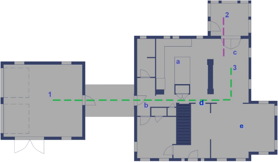Fig. 2 NZERTF diagram of the first floor. Instruments were located in (1) the garage, (2) the enclosed porch, or (3) the dining room. Locations for (a) cooking, (b) aged smoke injection, (c) chemical cocktail, and (d) fresh smoke. The pesticide was sprayed in (e) the living room. Other chemicals, including ozone (O₃), carbon dioxide (CO₂), and ammonia (NH₃), were injected directly into the supply air flow of the ventilation system (not shown). Dashed lines show sample lines from the garage (green) and porch (purple). Image created by Rileigh Robertson.

2.2 Study description

The experimental design of the CASA study focused on a series of physical and chemical perturbations to the test house, which was monitored by a suite of gas, aerosol, and surface measurements. Fig. 3 summarizes the experimental plan, which included physical environmental perturbations (changing temperature, RH, ventilation rate) and chemical perturbations (addition of wood smoke, commercial products, O₃, cooking emissions, etc.) to the house. Fig. 4 shows the schedule of experiments. Specific experiments are detailed in Sections 3.1–3.10 below. Table 1 shows average conditions for some of the indoor and outdoor measurements during CASA. Fig. S1† shows PM_2.5 concentrations measured by low-cost sensors in 12 locations inside the house and one outdoors. We express air levels of some chemical components as mixing ratios in parts-per notation defined as the number of moles of an analyte per mole of air, where parts per million (ppm) is μmol mol⁻¹, parts per billion (ppb) is nmol mol⁻¹, and parts per trillion (ppt) is pmol mol⁻¹.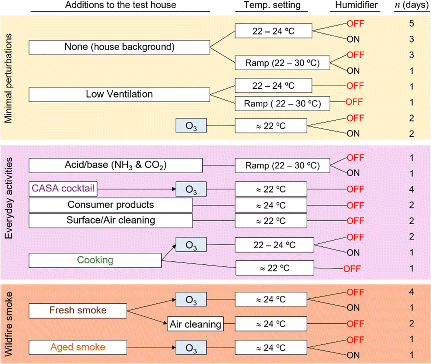

Fig. 3 The experimental matrix for CASA included perturbations to investigate the house during background conditions (yellow), additions of chemicals to represent both everyday indoor activities and the dynamic range of chemicals present indoors (pink), and additions of wildfire smoke (brown). Most experiments included replicates, and many were conducted under varying environmental or O₃ conditions. Stated temperatures represent typical ranges.

Fig. 4 The experimental schedule for CASA. Colors indicate the experimental categories described in Fig. 3: background days, changes in environmental conditions, and O₃ additions under background conditions are shown in yellow; everyday products and activities are shown in pink; and smoke additions are shown in brown. Ozone was injected in combination with almost all experimental conditions. The schedule reflects the dominant activity or condition for each day; several additional tests took place beyond those noted on this schedule (Section 3.10 for details).

Table 1 Campaign average indoor and outdoor conditions

	Indoor (average ± σ)	Outdoor (average ± σ)
a Average from first floor. Excludes temperature ramp and high RH tests.b Average excludes CO2 injections, average from basement, first and second floor.c Average excludes O3 injections and when there were high NO concentrations indoors.d Average from basement, first and second floor; attic average was 36 ± 5.2 ppb.e Average from basement, first and second floor; attic average was 161 ± 27.7 ppb.f Average from basement, first and second floor.g Average from dining area, from corrected PurpleAir measurements.h Average background measurements, excluding perturbations.i Average from outdoors on 11 April.
Temperature (°C)	24 ± 1 ^a	8 ± 6
Relative humidity^a (%)	32 ± 6 ^a	50 ± 20
Mechanical ventilation (m^3 h^−1)	250 ± 20	N/A
Air change rate (h^−1)	0.24 ± 0.04	N/A
CO2 (ppm)	500 ± 100 ^b	450 ± 30
O3 (ppb)	8 ± 1 ^c	31 ± 4
HCHO (ppb)	13 ± 5 ^d	1.2 ± 0.7
HCOOH (ppb)	30 ± 10 ^e	0.7 ± 0.3 ^e
NO (ppb)	1 ± 3 ^f	2 ± 7
NO2 (ppb)	4 ± 3 ^f	5 ± 6
PM2.5 (μg m^−3)	4 ± 20^g	3 ± 6
WSOCg (μg C m^−3)	220 ± 30^h	5 ± 1^i
WSOCp (μg C m^−3)	6 ± 3	Below LOD

---

2.3 Meteorological and trace gas data

Wind and temperature sensors, along with a pyranometer, collected meteorological data on the roof of the NZERTF.³⁴ Indoor house measurements included temperature in 20 locations, RH in seven locations, and air change rates from daily injections of SF₆ (Fig. S2†). Pitot tubes in the outdoor air, return, and exhaust ducts of the HRV provided mechanical ventilation air flow rates. A photoacoustic gas monitor provided CO₂ mixing ratios in five locations throughout the house and one location outdoors. Several trace gas monitoring instruments were placed in the passively-conditioned attic and shared an automated inlet switching system to sample air from the basement, first floor, second floor, attic and outdoors. These measurements included nitrogen oxides (NO_x), O₃, formaldehyde (HCHO), and formic acid (HCOOH). Total airborne water soluble organic carbon was measured on the first floor throughout the campaign, with one day of outdoor sampling. Additional reactive trace gas measurements included an array of organic and inorganic compounds, with inlet and instrument details in Section 2.4.

2.4 Instruments

Instruments were located in the house, attic, garage, and covered porch (Tables 2–4). Instruments in the garage and porch used inlet lines to sample from the dining room in the house; instruments in the house had short inlet lines, with most interior instruments located in the dining room. Several low-cost sensors were placed throughout the house. All gas-phase instruments had inlets made of 0.3625 cm (1/4′′) o.d. perfluoroalkoxy (PFA) tubing unless otherwise noted.

Table 2 Gas-phase and gas + particle phase instruments^a

Institution	Measurement	Instrument	Sample line/Instrument inlet details	Limit of detection (LOD) and time resolution	Comments
a Lpm = Liters per minute, PTFE = polytetrafluoroethylene, PFA = perfluoroalkoxy.
House trace gas system
National Institute of Standards and Technology (NIST)	CO2	Photoacoustic gas monitor	Sample line:3.2 mm (1/8′′) o.d. PTFE, <50 m	LOD: 1.5 ppm	Manifold system switching between six locations on a 4 min interval: First floor, second floor, basement, attic and outside
			Flowrate: 0.9 Lpm	Time resolution: 40 s
NIST	O3	Dual-cell, UV photometric	Sample line: 6.4 mm (¼′′) o.d. PFA, 9 m	LOD: 0.5 ppb	8-Port valve switching between five locations on 5 min intervals: outside, first floor, second floor, basement, attic
			Flowrate: 10 Lpm	Time resolution: 1 min
NIST	Formaldehyde (HCHO), formic acid (HCOOH)	Laser absorption spectrometer	Sample line: 6.4 mm (¼′′) o.d. PFA, 9 m	LOD:0.1 ppbv HCHO	Same as NIST O3 inlet
			Flowrate: 10 Lpm	Time resolution: 1 s
			Flowrate: 0.75 Lpm
Colorado State University (CSU)	NOx	Chemiluminescent detector with molybdenum oxide NO2 converter (Thermo Fisher model 42i TL)	Sample line: 6.4 mm (¼′′) o.d. PFA, 9 m	LOD: 2.3 ppb	Same as NIST O3 inlet
			Flowrate: 10 Lpm
Other trace gases
NIST	CO, CH4	Cavity ring down spectroscopy	No sample line	LOD: 5 ppb CO; 0.3 ppb CH4	Instrument was located in the dining room for a subset of experiments
			Flowrate: 0.07 Lpm	Time resolution: 3 s
CSU	SO2	Teledyne laser induced phosphorescence detector	No sample line	LOD: 0.5 ppb	Instrument was located in the dining room
University of California (UC) Berkeley	NH3, CO2, H2O, select VOCs	Cavity ring down spectroscopy, Picarro model SI9110	Sample line: 6.4 mm (¼′′) o.d. PTFE, 0.5 m	LOD: Ranges from 2 – 60 ppb	Instrument was located in the dining room
Massachusetts Institute of Technology (MIT)	VOCs	Low-cost VOC sensors (6 metal oxide, 3 electrochemical, 3 photo-ionization detectors)	Flowrate: 0.3 Lpm	LOD: Variable (sensor dependent)	Two units placed in kitchen, one with Nafion dryer inlet and one without; one unit placed in upstairs bedroom 3
			Sample line: 6.4 mm (¼”) o.d. PTFE, < 0.5 m	Time resolution: 1 s
MIT	CO	Infrared absorption gas monitor (Teledyne T300)	No inlet	LOD: 0.04 ppm	One unit placed in kitchen
				Time Resolution: 70 s
MIT	PM, CO	QuantAQ Modulair (low-cost sensor Node with Alphasense OPC N-3, Plantower PMS, Alphasense CO–B4 sensors)	No inlet	LOD: Variable	One unit placed in kitchen
				Time resolution: 5 s
University of Washington Bothell	Various	Low-cost indoor air quality monitor (AirAssure, TSI, Inc – O3, NO2, SO2, CO, CO2, VOC, PM)	No inlet	LOD: Variable	One unit place in kitchen
University of Toronto	VOCs	Proton transfer reaction mass spectrometer (PTR-MS) with gas chromatography	Heated inlet line: 6.4 mm (¼”) i.d. PFA tubing held at 50 °C, 30.5 m long	LOD: Variable	Calibrations and zeros performed every 3–6 h using a VOC mixed standard cylinder diluted in VOC-free air
			Flow rate: 4 Lpm through PTFE filter to scrub out particles	Time resolution: 4 s, averaged to 1 min	Operated largely in real-time mode, with periodic use of GC-PTR-MS mode
NIST	VOCs	PTR-MS	Heated inlet line: 6.4 mm (½′′) o.d. PFA tubing held at 50 °C, 30.5 m	LOD: Variable	Hourly zeros and calibrations using a VOC mixed standard cylinder diluted in VOC-free air. Operated only from 1 April to 11 April
			Flowrate: 5 Lpm through PTFE filter to scrub out particles	Time resolution: 1 s, averaged to 10 s	Operated exclusively in real-time mode
CSU	Oxidized organic and inorganic compounds	Time-of-flight chemical ionization mass spectrometer with iodide ionization (iodide-CIMS)^10,35	Same heated line as NIST PTR-MS	LOD: Variable	Hourly zeros and calibrations; mass resolution ≈4000 (m/Δm); 5 min outdoor sampling bihourly
				Time resolution: 1 s
Gas + particle instruments
University of North Carolina	Water soluble organic carbon in gas (WSOCg) and particle-phase (PM2.5; WSOCp)	Gas-phase with mist chamber (MC) (alternating with particle-phase by particle-into-liquid sampler, PILS^36), both analyzed with Sievers M9 total organic carbon analyzer	MC inlet: 9.5 mm (3/8′′) i.d. PTFE, 7.6 m	WSOCg & WSOCp alternate every 6 min	Sampling in dining room. Instrument in attached enclosed porch
			PILS inlet: 9.5 mm (3/8′′) o.d. Refrigeration-grade copper, 12 m	MC LOD: 0.5 μg-C m^−3	Daily blanks; MC collection efficiency measured for indoor WSOCg (data corrected) plus glyoxal, formic acid, acetic acid, acetone; PILS collection efficiency 95%^37
			PILS flowrate: 13 Lpm	PILS LOD: 2.0 μg-C m^−3	Precision: WSOCg 16%, WSOCp 10% ^38
				Time resolution: 4 s analysis time, 3.25 min response time	LOD limited by water background
UC Berkeley	Semi-volatile organic compounds (SVOC), typically organic compounds with vapor pressures C14–C30+ alkanes	Semi-volatile thermal Desorption gas Chromatography (SVTAG)^39	Sample line: 19.0 mm (¾′′) stainless steel, 1 m	LOD: Variable from high ppq to low ppt	Gas and/or particle measurements. Daily internal standard correction. Sampling through 2.5 μm cyclones and a denuder (for particle-only measurements)
			Flowrate: 10 Lpm	Time resolution: 1 h

---

Table 3 Particle-phase instrument summary

Institution	Measurement	Instrument	Sample LineInstrument inlet details	LOD and time resolution	Comments
CSU	Aerosol composition	High resolution time-of-flight Aerosol Mass Spectrometer^40 (AMS)	Two identical 15.9 mm (5/8′′) o.d. copper sample lines – one with an inlet in the dining room, the other with an inlet outside the garage; house sampling line temperature was maintained at 21 °C with heating tape	Time resolution: 5 s	Inlet alternated indoors (51 min) and outdoors (9 min)
CSU	Size distributions (27.4–723.4 nm)	Scanning mobility particle Sizer (SMPS, EC TSI 3080, DMA – TSI 3081, CPC – TSI 3010)	Same heated line as AMS	Time resolution: 3 min	Inlet passed through a silica bead diffusion dryer
University of Colorado (CU) Boulder	Size distributions (27.4–723.4 nm)	Scanning mobility particle Sizer (SMPS, EC – TSI 3082, DMA – TSI 3081, CPC – TSI 3750)	Same heated line as CSU	Time resolution: 3 min	Undried samples
NIST	Size distributions	Scanning mobility particle Sizer	No sample line
CU Boulder	Low-cost sensors	PurpleAir PA-II, 12 units distributed inside the house and 1 outdoors	No sample line	LOD: ≈1 μg m^−3 PM2.5	Each unit contains two Plantower PMS-5003 particle detectors
				50% at 0.3 μm, 98% at ≥0.5 μm
				Time resolution: 2 min
CU Boulder	Light absorbance	5-Wavelength aethalometer (MicroAeth MA 200)	Dining room	LOD: 30 ng m^−3
				Time resolution: 1 min

---

Table 4 Surface sampling and offline measurements

Institution	Sample type/collection approach	Sampling location	Measurement/instrument	Sampling notes
University of Michigan	Aerosol sample collection with Micro-Orifice Uniform Deposition Impactor (MOUDI)	Kitchen	Offline-AMS and Fourier Transform Ion Cyclotron Resonance Mass Spectrometry (FT-ICR)	Samples collected daily during activities
University of Michigan	Surface samples collected for off-line analysis	Kitchen, upstairs, living room	Offline-AMS and FT-ICR	Samples collected after activities over varying lengths (3 days to the full campaign)
University of California San Diego	Sample collection for off-line analysis	Kitchen	nanoIR2 (AFM-IR spectroscopy) with 30 nm spatial resolution	Samples collected daily
	In situ surface sampling	Kitchen	Quartz Crystal Microbalance (QCM)	Data collected every 6 s
	Sample collection for off-line analysis	Kitchen	ATR-FTIR (Model Nicolet iS50), Thermo Fisher Scientific	Samples were collected after cocktail, smoke, and other events
	Sample collection for off-line analysis	Kitchen	GC-MS (Thermo trace 1300/TSQ 8000 Evo Triple Quadrupole GC-MS)	Samples were collected before and after cocktail event
	Sample collection for off-line analysis	Kitchen	High-resolution mass spectrometer (Thermo Orbitrap Elite Hybrid MS)	Samples were collected before and after smoke event
Yale University	Sample collection for off-line analysis	Kitchen	Passive polydimethylsiloxane samplers for offline analysis of volatile and semi-volatile organic compounds via gas chromatography orbitrap high resolution mass spectrometry	Most samples were deployed before experimental days and collected prior to the subsequent experiment. Multiple samples were collected during cooking and smoke days
				Data can be used for targeted and non-targeted analysis
University of Toronto flux chamber	Surface fluxes of volatile organic compounds within an enclosed stainless steel chamber clamped to a painted windowsill	Windowsill on east-facing wall of house	PTR-MS measurements	30 minutes, spaced periodically throughout campaign
Multiple Universities	Vacuum floor dust samples for offline analysis	Entire house (first and second floor)	Various	Samples collected before and after smoke events

---

2.5 Safety considerations

All experiments and instrument deployments underwent review to determine potential for hazards or exposure concerns. Except for cleaning, cooking, and a subset of direct smoke and commercial product spray injections, no researchers were in the NZERTF during the experiments. The NZERTF was accessed daily to collect surface samples and check instrumentation located within the building envelope, but with at least 30 minutes between ending indoor activities and the start of the next perturbation.

3 Experimental details and selected findings

The CASA experiments can be divided into nine categories: house background, varying environmental parameters, ozone additions, smoke additions, air and surface cleaning, the CASA cocktail, product additions, acid/base additions, and cooking. An array of additional brief experiments were conducted throughout the project. Each group of experiments was designed to answer a specific set of questions. These questions, the subsequent experimental plan, and key data are presented below to demonstrate the chemical perturbation approach of the CASA study. Most perturbation experiments were compared to the house ‘background’ days described below. Finally, Section 3.11 summarizes the dust sample collection and subsequent microbial analysis that took place at the beginning and end of the project.

3.1 House background

The unperturbed house background includes measurements taken while no people were in the house and in the absence of intentional activities or perturbations. All exterior doors and windows remained closed. The balanced ventilation and exhaust system was set to 250 m³ h⁻¹. The indoor blower of the two-stage heat pump operated continuously while its compressor cycled on, as needed, to maintain the first floor temperature at the 24 °C setpoint. The whole house humidifiers were disabled for most background days, but operated for several consecutive hours on three background days. The house background thus includes influences from emissions of building materials, infiltration of outdoor air, HVAC system operation, and other automated activities including the dishwasher, clothes washer, clothes dryer and bathroom water lines that were automatically turned on and off on a predetermined schedule. CASA included five full days of ‘house background’, spread across the entire project, plus three days with elevated humidity and four days of ramped temperature setpoints at either high or low humidity. On two additional days (April 9 and 10), the fixed, continuous mechanical ventilation rate was decreased from the typical rate of 250 m³ h⁻¹ (150 cfm) to 50 m³ h⁻¹ (30 cfm); the first low-ventilation day included a temperature ramp. On some background days, individuals were present in the house for short periods of time for maintenance activities.

Specific science questions investigated during the house background conditions included:

• What are the influences from building material emissions and outdoor air infiltration into indoor air?

• How does the cycling of HVAC and other indoor automated activities (e.g., dishwasher and clothes washer) affect the composition of indoor air?

• How do changes in ventilation conditions, indoor temperature, and humidity change indoor chemical composition of gases, particles, and surfaces?

These background periods enabled analysis of how outdoor pollution impacted indoor air. For example, Link et al.⁴¹ used the CASA data and a chemical box model to show that nitric oxide (NO) of outdoor origin could titrate the low levels of indoor O₃ and inhibit the production of indoor NO₃.

3.2 Environmental parameters

These perturbation experiments included days in which RH, temperature, or ventilation rates were varied from the background house conditions. These three parameters can be mechanically controlled in residences and affect human comfort and health. However, these environmental parameters may also affect chemical processes in a house. For example, temperature influences the partitioning of semi-volatile species between surfaces or particles and air, as well as chemical reaction rates. Air concentrations of phthalates correlate with indoor temperature, demonstrating a link between thermal comfort and indoor air composition.⁴² Increased ventilation reduces indoor air pollutant concentrations if the outdoor air is lower in concentration than indoor air, or if the air is treated in a mechanical ventilation system to reduce, for example, particulate matter or O₃.

During the COVID-19 pandemic, recommendations for increased ventilation aimed to reduce respiratory aerosol concentrations. However, when ventilation dilutes indoor air with outdoor air, shifts in surface-air partitioning can drive semi-volatile compounds from surface reservoirs into the indoor air. Wang et al. provide an example of this dilution-driven partitioning from the HOMEChem study, in which concentrations of semi-volatile organic compounds decreased during enhanced ventilation events, but increased once the enhanced ventilation was stopped and the house returned to normal operation.¹⁵

Relative humidity also impacts indoor concentrations, causing increased liquid water content of surfaces and aerosol, thus enhancing uptake of water-soluble compounds^43,44 and potentially enabling aqueous chemical reactions. Water vapor may also react with compounds in the air, including carbonyl oxide intermediates created from ozonolysis of alkenes.⁴⁵ Additionally, water vapor may displace other molecules on surfaces and shift surface-air partitioning. Water vapor leads to hygroscopic aerosol growth, increasing aerosol mass and size, and thus influencing deposition rates – both within a building and within the human respiratory system. However, the extent of these transformations in the indoor environment, and their potential impacts on air toxics and other chemical contaminants, surface chemical reservoirs, or human health are poorly constrained.

The CASA study included multiple manipulations of the house systems to investigate how environmental parameters impact chemical processes in the indoor environment. Specific questions of interest included:

• What is the pool of semi-volatile organic and inorganic components in indoor surface reservoirs?

• To what extent can temperature changes influence indoor chemical composition of gases, particles, and surfaces?

• How do surfaces and particles take up water?

• How do the concentrations of water soluble gases change with humidity?

Under background “low RH” conditions, humidifiers were kept off and the average RH was 32%, but ranged between 30 and 50%. On high RH days, the whole house in-duct humidifiers were turned on and set to their maximum speed. On these high RH days, the temperature typically increased from the 24 °C setpoint to about 27 °C and RH increased to about 70% RH. Each high RH day was paired with an identically scripted low RH day (i.e., humidifiers off) day. These paired RH perturbation days included:

• Background conditions (one high RH versus nine low RH days).

• O₃ additions (two high RH versus two low RH days).

• Cooking (one high RH versus two low RH days).

• Temperature ramps (one high RH versus one low RH day).

• Acid-base additions (one high RH versus one low RH day).

• Fresh smoke additions (one high RH versus three low RH days).

• Aged smoke additions (one high RH versus one low RH day).

Because of the auxiliary resistive heating coupled with the refrigerant-based heat pump heating, the NZERTF can be heated much more quickly than it can be cooled. Moreover, a target humidity level, especially a higher one like that used for CASA high RH days, can be sufficiently controlled when increasing the NZERTF's dry bulb temperature. Reducing the indoor temperature while maintaining a target humidity level was beyond the capabilities of this house. Consequently, all temperature ramps conducted during CASA progressed in one direction, from coolest to warmest. Prior to starting a temperature ramp, the house was cooled to between 18 and 20 °C. The system was then switched to heating while maintaining continuous indoor blower operation. The house was heated by 2 °C increments from 20 to 30 °C; each temperature step was maintained for approximately two hours. Overall, the entire six-step temperature ramp took approximately eighteen hours to complete. A few hours were needed before temperatures returned to the background conditions of 24 °C. Temperature ramps were conducted at normal low RH (5 March), high RH (19 March), and low ventilation (9 April) conditions. This low ventilation temperature ramp was the sole experiment conducted during CASA at different ventilation conditions. Additional experiments were conducted with a limited subset of instrumentation after the end of the CASA experiment.

We observed that environmental parameters influenced indoor SVOC concentration. During a temperature ramp with RH held at 40%, each 1 °C rise in temperature corresponded to an increase in SVOC concentration by about 25% with respect to the house background signal (Fig. S3†). In comparison, during the high RH day (80% RH), each 1 °C rise in temperature corresponded to an increase in the SVOC concentration by about 50% of the background sample signal. Thus, RH plays a significant role in modulating SVOC concentrations in indoor air and may even enhance the temperature-dependent partitioning for certain compounds.

Further evidence that multiple processes control surface-gas exchange comes from temperature ramps on low RH versus high RH days. We observed that many gas-phase SVOCs were consistently higher in concentration under higher humidity conditions (80% RH) compared to background (≈32% RH). While temperature varied on high RH days, the SVOCs are more clearly linked to changes in RH. Fig. 5 shows that during a high RH event, the more volatile SVOCs, such as the C_8–10 carboxylic acids, increase in gas-phase concentration. This response is weaker, but still apparent, for alkanes with similar volatility (C_12–16) indicating that volatility is not the only factor driving this humidity effect. We hypothesize that water molecules compete with active sorption sites on surfaces when the humidity is increased, thus liberating some of these SVOC molecules. Some SVOC species, such as levoglucosan and vanillic acid/vanillin (not shown here), show no dependence on RH.

Fig. 5 Signal from the SV-TAG during smoke additions conducted under changing RH. The signal has been normalized to the greatest signal intensity and is shown as an enhancement to the house background sample (27 March 1:00 AM). Relative humidity and temperature are shown in the dashed black and solid grey lines respectively. Black arrows correspond to fresh or aged smoke injections. Various cleaning, filtering, and ozone additions occurred on 28 March, which results in some variability in the signal.

3.3 Ozone additions

Ozone is a well-studied oxidant in the indoor environment that can react with unsaturated organic compounds on surfaces and in air. During CASA, indoor O₃ averaged 8 ± 1 ppb with an average indoor to outdoor concentration ratio of 0.26, in line with other North American residential environments.^9,14,46,47 Indoor levels are typically much lower than outdoor levels due to high indoor reactivity. One recent study indicated that ozonolysis products from squalene, a reactive component of human skin oil, can be persistent indoors.¹⁴ The addition of ozone to indoor environments can also contribute to secondary organic aerosol.⁴⁸ However, the extent to which indoor ozonolysis contributes to secondary air pollutants formed indoors is poorly quantified. To this end, two types of O₃ perturbations were conducted during the CASA study: extended O₃ additions (longer releases of O₃ of 60–180 minutes peaking 80 ppb on the first floor) and punctuated O₃ additions (short bursts in O₃ release with indoor concentrations rising to 60 ppb within 30 minutes). The mass of O₃ injected was not equal during these two experiment types. However, these two contrasting approaches enable studies of both multigenerational oxidation chemistry from longer exposures, and first order decay time analyses from shorter exposures.

Ozone additions were designed to mimic the enhancement of ozone, though not the levels of other pollutants, upon opening a window on a high-O₃ day. The O₃ injection system was comprised of a cylinder of high-purity oxygen (O₂) and a remotely-controlled two-way solenoid valve from the regulator to a mass flow controller on the porch of the test house. The mass flow controller, also located in the enclosed porch, delivered the O₂ to an O₃ generator at a flowrate of ≈1 Lpm. The power supply for the high-voltage O₃ generator was also remotely controlled. Ozone from the generator transferred through a 3.2 mm (1/8′′) PTFE line to the HRV supply duct in the basement of the test house. The HRV supply duct distributed air to the dining room on the first floor and to each of the second floor bedrooms. The HRV flows between the first and second floors were not perfectly balanced, and the mass of O₃ delivered to these spaces may have been slightly different.

Ozone addition experiments were performed periodically throughout the CASA study to investigate the following questions:

• What is the fate of O₃ in the built environment, and to what extent can outdoor ozone impact indoor air quality?

• Does the house's reactivity to O₃ change with time, or after O₃ exposure?

• What are the main O₃ products and their kinetics following both chemical perturbations and changes in environmental parameters?

Four punctuated O₃ injections caused increased concentrations in the main spaces of the test house (first and second floors), while only changing slightly in the basement, and not changing at all in the attic or outdoors (Fig. 6). A key finding from O₃ addition experiments was that adding ozone enabled formation of NO₃ radicals following oxidation of ambient NO₂; these NO₃ radicals could then initiate oxidation reactions that impacted VOCs and generated organic nitrate products – highlighting the problems with adding ozone to buildings.⁴¹

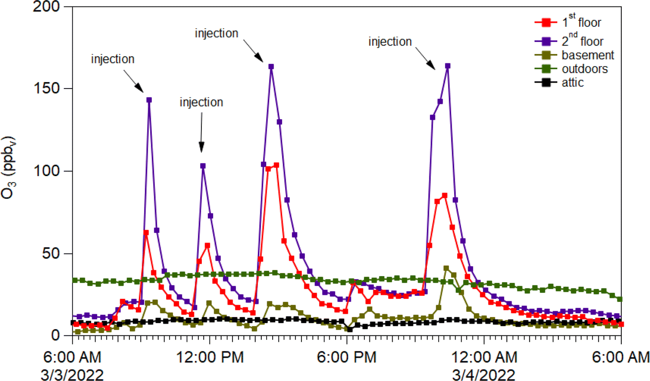Fig. 6 Ozone concentrations (ppb) on 3 March 2022 as detected from inlet lines located on the 1st (red), 2nd (purple), and basement (brown) floors in contrast to the outdoor (green) concentrations.

In one subset of ozone addition experiments, we diluted the inflow to the O₃ generator with ≈10% of ¹⁸O-labeled O₂. ¹⁸O is a rare stable isotope, and its addition was observed in secondary reaction products observed by the iodide CIMS, with an ¹⁸O enhancement on the order of the same ratio as the injection ozone (11%, Fig. 7a). The presence of ¹⁸O-labeled N₂O₅ (Fig. 7b) directly demonstrates that O₃ reacts with NO₂ indoors to form N₂O₅. N₂O₅ is well established to react with aerosol surfaces to form HNO₃, providing a potential mechanism for infiltration or addition of O₃ pollution to acidify indoor surfaces.

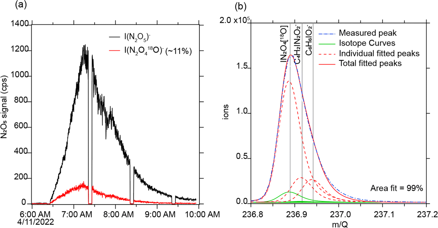Fig. 7 (a) Adding labeled O₃ to the house enhanced ¹⁸O–N₂O₅. (b) The I-CIMS separates ¹⁸O-substituted N₂O₅ from adjacent ion peaks in the mass spectrum. Note that the timeseries includes periodic zero air measurements; signals decrease during this time.

3.4 Smoke additions

Over the last few decades, wildfires have increased in frequency across the western United States, raising concerns over their influence on outdoor air quality and public health.^29,49 Smoke is a complex mixture including both particulate matter and trace gases. While concentrations of particulate matter are typically lower indoors than outdoors during poor air quality events, indoor concentrations can still reach levels of concern.^30,31 Further, the influx of outdoor air pollution to the built environment, either through door or window opening, mechanical ventilation, or leaks in the building envelope, may add new chemical compounds to the indoor chemical system and induce secondary chemical transformations. Residential wood burning also introduces smoke compounds in the gas or particle phase into the indoor environment. The extent to which wood smoke in buildings can impact human exposure to various chemical contaminants on timescales beyond the outdoor pollution event is poorly understood. For example, recent wildfires at the wildland–urban interface have raised concerns about smoke damage to indoor spaces and the efficacy of different mitigation approaches.⁵⁰ Wildfire events are not the only sources of wood smoke to indoor environments: wood stoves and fireplaces can directly release smoke to the indoor environment,⁵¹ while simultaneously releasing smoke to the local area, potentially impacting other homes.

The CASA study provided an opportunity to investigate how wood smoke impacts indoor chemistry. Specific questions of interest included:

• Where does smoke go in a house (i.e., deposition versus ventilation versus reactive chemistry), and how does it chemically transform on the timescales of air change rates?

• Do deposited smoke compounds undergo chemical reactions, and on what timescales?

• How does smoke interact with ozone? How does humidity impact smoke and resulting surface soiling?

Introducing fresh wood smoke to a house involves two challenges: first, safely and consistently making smoke that is chemically comparable to wood smoke, and second, introducing the smoke into the house in a reproducible manner. At CASA, we used a portable cocktail smoker (Breville, “the Smoking Gun”, BSM600SILUSC), loaded with Ponderosa pine woodchips to generate wood smoke. This smoke was then added either directly to the house as bursts of fresh smoke, or to an outdoor chamber where it was oxidized by ozone and then injected to the house as simulated aged smoke.

For fresh smoke, a fixed amount of wood chips (about 0.5 g per event) was added to the cocktail smoker inside the house, which then directly released smoke into the house near the kitchen. To simulate aged smoke, we first added large levels of O₃ to an approximately 1 m³ Teflon chamber located outside of the house between the garage and the house (chamber mixing ratios on order of 20 ppm O₃). Smoke was then added to the chamber by processing about 6 g of woodchips. The O₃ and smoke-filled chamber was then left undisturbed with no air flow in or out for 45 minutes. To inject the aged smoke into the house, a second valved port on the chamber was connected to a short length of copper tubing that originated from just inside the house while being routed through a fixed partition which, during CASA, had replaced the house's west-side exterior door. Having connected a zero air (Environics, Series 7000) source to the chamber via the tubing previously used for O₃, valves within the inlet and outlet ports were opened while flowing air into the chamber at a rate of about 20 Lpm for 40 minutes. A fan located inside the house, next to the inlet from the smoke chamber, was remotely turned on during the addition to increase mixing, and concentrations of particulate matter and other smoke markers immediately increased. After 30–40 minutes, particulate matter concentrations in the house leveled off, indicating that the bulk of the aged smoke had entered the house. Despite the high levels of ozone used in the chamber, ozone did not increase in the house during injections of aged smoke. Smoke experiments took place in the latter part of the CASA study to ensure that any changes to the background did not influence other experiments. As discussed by Li et al.,⁵² we found that smoke VOCs partitioned to surfaces of the house and were released back into the house over hours to months timescales, which are longer than the house's air change rate timescale.

Peak indoor PM_2.5 concentrations were 120 ± 40 μg m⁻³ for fresh smoke additions and 150 ± 50 μg m⁻³ for simulated aged smoke additions. The fresh smoke PM_2.5 was dominated by submicron particles, while the aged smoke PM_2.5 was primarily composed of supermicron particles, likely due to the aging process in the ozone chamber. On low RH days, fresh smoke injections led to higher concentrations of brown carbon compared to simulated aged smoke, while concentrations of black carbon were similar between fresh and aged smoke additions (Fig. 8).

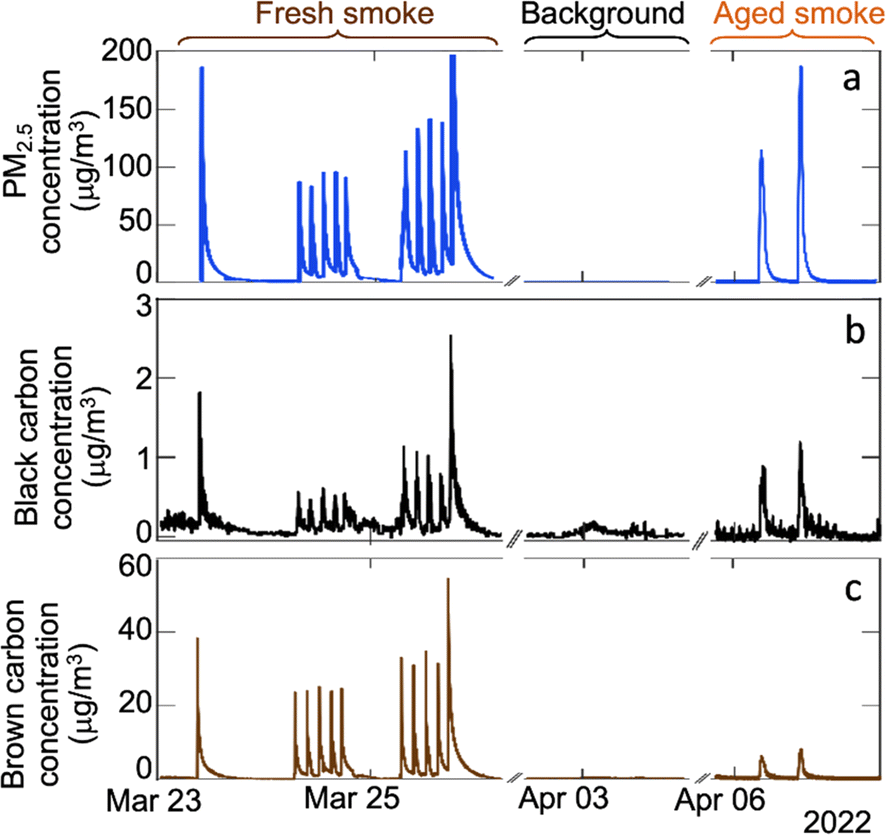Fig. 8 (a) Indoor PM_2.5 concentrations obtained from combined SMPS (electrical mobility diameter = 24.4–723.4 nm) and APS (aerodynamic diameter = 0.7–2.5 μm) measurements assuming a density of 1.2 g cm⁻³, (b) black carbon, and (c) brown carbon concentrations from aethalometer measurements from fresh smoke additions (23–25 March), house background (2–3 April) and simulated aged smoke additions (6–7 April). Note that the y axes have different scales between panels. The EPA's optimized noise-reduction algorithm was applied; MAC values for the analysis were 24.1, 19.1, 17.0, 14.1, and 10.1 at wavelengths of 375, 470, 528, 625, and 880 nm, respectively.⁵³ Aethalometer data was not analyzed during high RH days because humidity causes significant interference in those measurements.

The bulk organic chemical composition of the aerosol produced from the cocktail smoker is similar to that observed in western wildfires. Li et al.⁵² compared the mass spectrum of the submicron non-refractory smoke aerosol directly output from the cocktail smoker to wildfire smoke measured during the WE-CAN 2018 study, in which we previously collected ambient aerosol data on an aircraft flying through wildfire plumes in the Western United States.⁵⁴ The aerosol mass spectra are very similar (r² = 0.90),⁵² with the key exceptions being in particulate nitrate. The relatively low temperature of the cocktail smoker is designed to maximize smoke generation and minimize flaming, which results in negligible NO_x and HONO, and hence a lower generation of particulate nitrate. However, submicron aerosol in wildfire smoke is dominantly (85–96%) organic, and the cocktail smoker appears to be an adequate generation device for simulated wildfire smoke. In terms of gas-phase emissions, the emissions ratios for key VOCs (formaldehyde, benzene, toluene, formic acid, acetic acid, acetone, furan) relative to CO agreed to within an order of magnitude of the western wildfire smoke plumes sampled during WE-CAN (Fig. S4†).⁵⁵ However, emissions ratios for pyrrole were an order of magnitude larger, and emissions of acetonitrile were an order of magnitude lower, for CASA than at WE-CAN. We thus take the smoke generated by the cocktail smoker to be a useful simulation of wildfire smoke for this project.

Smoke components deposit on indoor surfaces, with the deposited particles showing surprisingly complex morphology and composition. We investigated this deposition and subsequent chemistry through off-line microspectroscopic analysis of window glass samples that were placed both vertically and horizontally in the kitchen and living room area for 24 hours before, during, and after a smoke injection experiment. Upon collection, samples were sealed and subsequently analyzed using atomic force microscopy-infrared (AFM-IR) spectroscopy (Fig. 9). Two different types of particle morphologies were identified on exposed glass surfaces: (1) aggregate-like (Fig. 9a) and (2) rounded (Fig. 9b). The aggregate-like smoke particles were much larger, taller, and rougher than the rounded particles – similar to ash. Aggregate-like particles were up to 2.6 μm in height, while rounded particles were <100 nm in height.

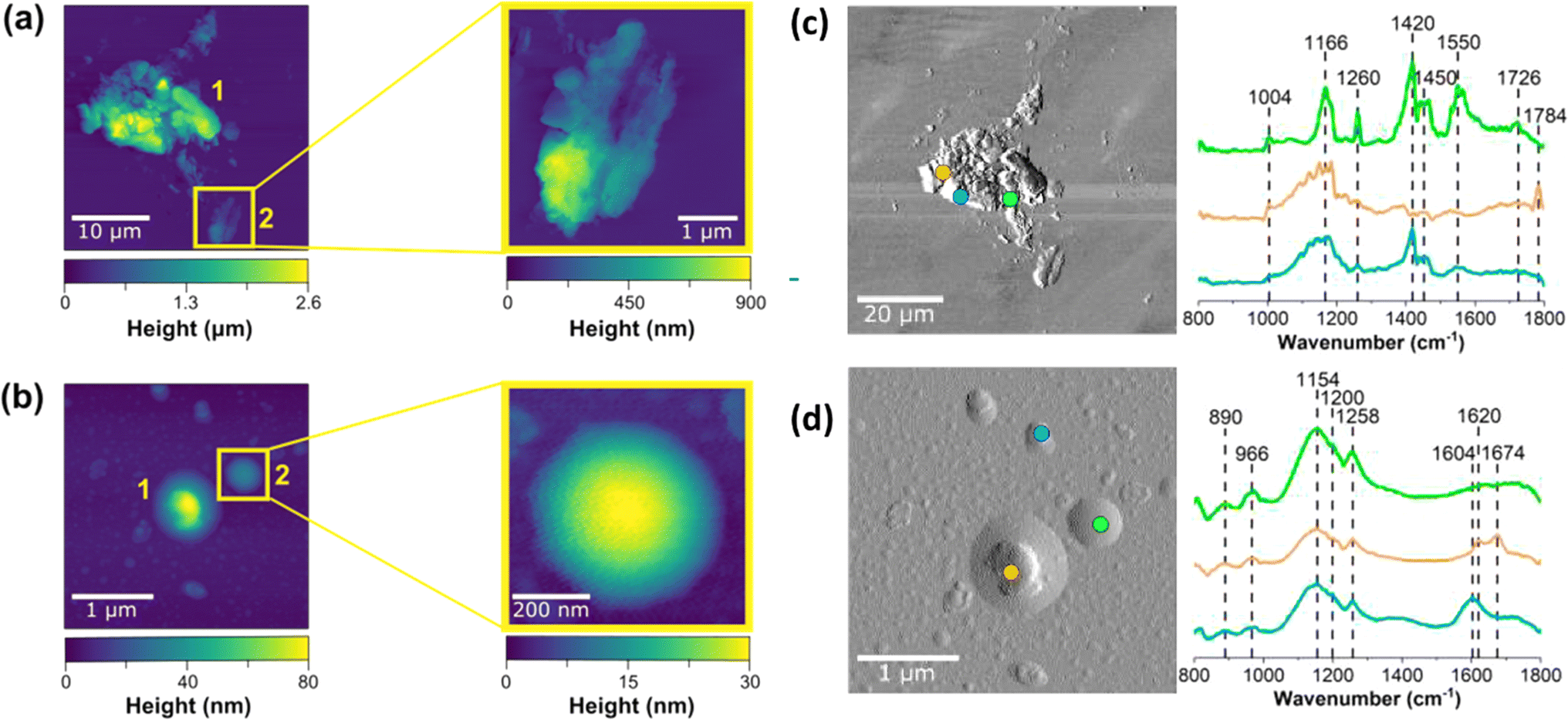Fig. 9 AFM 2D height images of smoke particle deposition on glass in two different regions on the surface of two different particle morphologies – (a) aggregate-like particles and (b) rounded particles. The left side represents a height image for a larger region, while the right side is a zoomed-in height image. (c) and (d) are the corresponding deflection images along with AFM-IR point spectra. Each spectrum was obtained by co-averaging seven spectra on the same point as shown by the colored dots in the deflection image and the color-coded spectra. All infrared spectra were collected at 100% power in tapping mode. AFM images were processed using the Gwyddion software; AFM-IR spectra were plotted in Origin.

The two particle types (aggregate-like vs. rounded particles) are not only morphologically distinct, but also chemically distinct. As shown in the deflection images for aggregate-like and rounded particles, point spectra were collected in different regions of each of the particle types. For example, the blue and orange spectra shown in Fig. 9 have broad peaks around 1166 cm⁻¹, which can be associated with C–O stretching found in esters, C–O–C stretching, or potentially sulfate derivatives.⁵⁶ Spectra shown in blue and green also have a distinct peak at 1420 cm⁻¹, consistent with aliphatic carbon chains from sugars in the wood. The spectrum shown in orange also has a very distinctive peak centered around 1784 cm⁻¹ associated with the C=O stretching motion of esters. The spectrum shown in green also has a peak above 1700 cm⁻¹ associated with protonated C=O in protonated carboxylic acids, whereas the two peaks at 1500 and 1450 cm⁻¹ are indicative of carboxylate stretching motions. The three different observed spectra on a single aggregate thus clearly depict the complexity of these samples and provide evidence for the presence of multiple functional groups within a single aggregate-like particle. In contrast, rounded smoke particles exhibit more consistent spectra with broad bands ranging from 1000 cm⁻¹ to 1300 cm⁻¹, indicative of C–C and O–H functional groups that are commonly present in biomass burning aerosol, including levoglucosan or catechol.^57,58 Peaks at 1604 cm⁻¹, 1620 cm⁻¹ and 1674 cm⁻¹ suggest the presence of aromatic, unsaturated C=C, and aldehyde functional groups, respectively.^56,58–60 Although more analysis is necessary to fully characterize these smoke-deposited aerosols, these data provide microscopic evidence for the deposition of smoke particles on window glass surfaces that vary in not only size and morphology, but also in composition.

3.4.1 Post-smoke ozone injections. Wildfire smoke events are often associated with elevated ozone levels in urban environments due to secondary chemistry induced by the combination of wildfire smoke and anthropogenic urban emissions.^61,62 Further, ozone is commercially used to reduce indoor smoke odors, although the bulk of the scientific literature on ozone reactions with smoke in indoor environments focuses on cigarette smoke.⁶³ In order to evaluate how a smoke-contaminated building responds to ozone, we conducted a suite of experiments in which ozone was injected into the house 1 to 2 hours after either direct or aged smoke additions. Results from these experiments will be discussed in future manuscripts.

3.5 Air and surface cleaning

CASA included both surface cleaning (vacuuming, dusting, mopping) and use of portable air cleaners. Cleaning includes both the addition of commercial or homemade products with the aim of removing soluble or mobile contaminants, and the direct removal of dust and other potentially harmful components present in an indoor space. Cleaning products are well-established to release inorganic and organic compounds into indoor air,^27,35,64 leave residue on indoor surfaces,⁶⁵ and have unintended effects on indoor chemistry. For example, the addition of bleach solutions can induce multiphase chemistry,^35,64,66 while the addition of hydrogen peroxide can induce formation of hydroxyl radicals and other oxidants.^67,68 Persistent organic pollutants and several other chemical contaminants are well-established to adsorb and accumulate on dust surfaces,⁶⁹ meaning that dust removal is a potentially effective tool to reduce exposure to harmful contaminants – not to mention allergens, bioparticles, and other indoor solid-phase pollutants. While most cleaning is focused on surfaces, air cleaning is growing in interest, particularly in light of the broad recognition of airborne pathogens during the COVID-19 pandemic. Air cleaners generally use physical or chemical techniques to remove air pollutants. Physical approaches include filtration or removal by other adsorptive substances to physically extract particulate matter or volatile organic compounds from air. Chemical approaches to air cleaning include the use of ultraviolet light, photocatalytic oxidation, ions, or oxidants such as hydrogen peroxide or hypochlorous acid to destroy pathogens, induce deposition of particulate matter, or chemically transform other chemical air contaminants. While use of filters is well-established in the scientific literature, chemical air cleaning techniques are less well understood and potentially subject to unintended chemical consequences.²³ Surface cleaning at CASA was limited to two specific events – one just prior to the first smoke additions on 21 March, and one at the end of the smoke additions on 7 April. These two surface cleaning events included manually vacuuming the floors and dusting all horizontal surfaces on the first floor of the house, shortly followed by mopping and surface cleaning with an aqueous cleaning mixture. The aqueous mixture was based on the Red Cross recommendation for cleaning after wildfire smoke events, and included a scented cleaning product mixed to manufacturer instructions, along with trisodium phosphate (4 tbsp of trisodium phosphate, 1 cup of cleaner, 1 gallon of water). We collected dust and other residue from the vacuum cleaner (116 g prior to smoke events; 35 g after smoke events), which were stored in a refrigerator or freezer for off-line analyses.

To assess the efficacy of various air cleaners, four consumer-grade portable air cleaners were procured from different manufacturers with prices ranging between $500 and $1000. These air cleaners were chosen to cover a broad spectrum of physical and cleaning technologies, including dual polarity ions, photocatalytic oxidation (PCO), UV, electrostatic charge, HEPA filter, and activated carbon filter. Additionally, two custom-built Corsi-Rosenthal boxes⁷⁰ were tested, one with MERV-13 filters and the other with combined activated carbon and MERV-8 filters. All air cleaners were situated in the dining and kitchen area during operation.

These cleaning events allowed us to investigate:

• Can surface cleaning affect indoor air before and after simulated wildfire smoke additions?

• How effective are surface versus air cleaning approaches to cleaning indoor air?

• Does the indoor dust and microbial composition change before and after wildfire smoke events?

• How effective are common portable air cleaners at removing particulate matter and volatile organic compounds?

• Do portable air cleaners induce secondary chemistry with observable effects on indoor air composition?

Results from these experiments will be discussed in future manuscripts

3.6 CASA cocktail

To investigate how the fate of organic compounds varies with molecular properties, we injected a gaseous mixture of compounds covering a range of volatilities and organic functional groups into the house. The injection represented a rapid pulse (e.g., from sudden infiltration of outdoor air or short-term emission from indoor sources). This mixture – the ‘CASA cocktail’ – comprised 1-hexene, 1-octene, isoprene, α-pinene, toluene-d8, acetone, 2-pentanone, chlorobenzene, o-xylene, 2-heptanone, and furfural; these compounds were selected to represent specific chemicals or structural features of interest in the indoor environment. The experiment was performed five times: during the first four trials, 0.34–0.55 g of each species was injected to the house, and during the fifth trial, this was diluted by a factor of 10 such that 0.034–0.055 g of each was added. To ensure the mixture was injected in the gas-phase, we heated the mixture in a water bath on a hot plate at 90 °C, passing zero air through the mixture in a bubbler at 10 Lpm and into a port on the porch door. The mixture took, on average, eight minutes to evaporate, during which time a box fan near the inlet in the dining room was remotely turned on. Following addition of the CASA cocktail to the house, no personnel entered the house, nor were other activities conducted for at least five hours. For half of the CASA cocktail experiments, ozone was injected at the six-hour mark, while for the other half of the experiments, the CASA cocktail was left to decay over twelve uninterrupted hours with no ozone addition.

The CASA cocktail experiment allowed us to investigate the following science questions, among others:

• How does the temporal behavior and fate of indoor pollutants vary with their molecular properties?

• How do differences in volatility and the presence of functional groups affect indoor VOC sorption on different building materials?

During the CASA cocktail experiment, we deployed thin, porous films of varying building materials on a horizontal glass slide in the dining room collection area. These materials included clay (kaolinite), commercial zeolite, cement (CaO + CaCO₃ mixture) and rutile (TiO₂). These porous films were exposed to the CASA cocktail and then sealed and stored refrigerated prior to shipping to UC San Diego. Any organic compounds that remained adsorbed on or within the thin film were extracted with acetone and analyzed by GC-MS and compared to a glass slide with no porous film coatings (Fig. 10a). The instrument was operated using a TG-WAXMS column (30 m × 0.25 mm i.d. × 0.25 μm film thickness, Thermo Scientific) with the injection temperature of 230 °C and the following oven temperature program: 40 °C for 3 min, then gradually increased to 230 °C at a rate of 15 °C min⁻¹, and the final temperature was held for 10 min. The identification of adsorbed surface products was based on the NIST electron ionization mass spectral library. Most interestingly, 1-octene adsorbed strongly on several – but not all – of the surfaces. Glass showed little to no surface product, whereas kaolinite showed the highest adsorption of 1-octene and the formation of oxidized products of the cocktail gases including oxidized α-pinene. Other reactive surfaces included cement and titanium dioxide. This outcome suggests that CASA cocktail precursor compounds did transform on indoor-relevant surfaces as some of the surface products were unique from the gas-phase precursors and varied according to surface type.

Fig. 10 (a) Extracted organic compounds from different surfaces deployed during the CASA cocktail experiment as detected by GC-MS. (b) Attenuated Total Reflection Fourier Transform Infrared spectroscopic data of organic compounds on a TiO₂ surface collected during the CASA cocktail experiment.

In addition, a TiO₂ thin film deposited on an Attenuated Total Reflection element (ATR) was analyzed with FTIR spectroscopy (Fig. 10b). The ATR data show vibrational frequencies consistent with alkenes, aromatics, and carbonyls. Taken together, the ATR and GC-MS data demonstrate that different building materials retain and potentially react differently with gas-phase species. For some materials, there is no adsorption or product formation, while in others, adsorption and product formation are evident.

3.7 Product addition

Where the CASA cocktail experiment focused on a curated suite of VOCs, commercial products include complex mixtures that can be released in the indoor environment through spray cans. The fate of such commercial products and the mechanisms by which they can contribute to human exposure are poorly understood. Spray cans are typically expected to release large particles that rapidly deposit to surfaces. Insecticides are lower-volatility compounds; however, these lower-volatility components could enter the gas-phase and partition either to surfaces or to preexisting indoor aerosol particles. We sprayed a commercially available flying insect pesticide containing permethrin and tetramethrin as active ingredients in the living room of the house for 25 seconds in accordance with manufacturer instructions. This spray time corresponded to a product mass loss of about 30 g from the bottle. A box fan in the living room that directed air towards the living/dining room area was turned on two minutes prior to the start of the spray, and turned off four minutes after the event. According to the manufacturer, the insecticide contained 0.15% permethrin, 0.15% tetramethrin, and 99.70% ‘other ingredients’ including isobutane, propane, hydrotreated light petroleum distillates, and light aromatic solvent naptha from petroleum.

This insecticide addition allowed us to investigate:

• What is the chemical behavior of low-volatility consumer product sprays in indoor air and surfaces?

• What is the timescale of the different components in the insecticide spray in the indoor air?

Results from this experiment will be discussed in detail in a forthcoming manuscript.

3.8 Acid/base addition

Surfaces play a major role in indoor chemistry, in part because sorption to abundant indoor surfaces prolongs the indoor residence time of compounds, providing more time for reactions to take place. There is evidence that sufficient surface-bound water can exist on soiled indoor surfaces to enable the uptake of water-soluble gases⁷¹ and studies of surface-bound tobacco smoke suggest that changes in surface pH can alter the gas-surface partitioning of indoor contaminants.^72,73 However, the degree to which variations in pH in surface water reservoirs affects most indoor species is poorly understood. To approach this topic, we asked:

• How does the intentional introduction of a weak acid gas (CO₂) or base gas (NH₃) influence the dynamic concentrations of water-soluble organic compounds, target organic acids and bases and other target species?

• How do the effects of acid-base additions vary with RH?

In these experiments, CO₂ or NH₃ was injected into the supply air flow of the mechanical ventilation system for about 30 minutes (500 g min⁻¹ CO₂; about 40 mg min⁻¹ NH₃) with the goal of reaching mixing ratios that were high but realistic (on the order of 5000 ppm CO₂ and 500 ppb NH₃). They were then allowed to decay for at least 3 h. The process was repeated three to four more times. The first day involved injections at high RH, while the second day involved injections at background RH.

NH₃ decayed faster than the air change rate due to surface uptake. We measured about 20% lower mixing ratios of NH₃ at high RH, suggesting enhanced surface removal into sorbed water. We observed various gas-phase bases or acids increase following injection of CO₂ or NH₃, likely due to shifts in the pH of surface water reservoirs. High RH likely increased the surface reservoir of water, thereby enhancing the impact on more water-soluble aids and bases. Results will be presented in detail in forthcoming manuscripts.

3.9 Cooking

Cooking experiments investigated the following questions:

• How are particles emitted from cooking in the kitchen transported throughout the house and how does the transport timescale compare to the air change rate?

• How do cooking emissions and resulting surface/particle/air contributions change between high and low RH conditions?

• Is the water uptake of cooking emissions different from that of smoke?

• How do cooking emissions change as particles and gases get transported throughout the house?

• How do cooking emissions interact with ozone?

The NZERTF used for CASA lacks any combustion-based appliances (e.g., natural gas). We used a two-burner electric cooktop at maximum setting and an electric air fryer for cooking experiments, which took place over a 3 day period from March 13 to 15. The first day of experiments was performed at high RH (60–80% on the first floor, slightly lower upstairs) and the other two days at low RH (30–50%). Eight cooking experiments were performed in these three days involving the same ingredients and preparation. Six of these were done on a frying pan while the other two were conducted with an air fryer. The cooking process consisted of heating up the pan or air fryer with canola oil (10 g for pan fryer), then sequentially adding vegetables, frozen potato products, and bacon; each food item was cooked for ten minutes. Specific details for all cooking events are in Table S1.† At the conclusion of each cooking event, the cook removed all food from the test house. Fig. 11 shows the average particle number size distributions measured during air frying and pan cooking, demonstrating that air frying released a larger amount of smaller aerosol particles compared to pan cooking for similar meal preparations and same ingredients.

Fig. 11 Average particle size distributions sampled in the dining room during all air frying and pan cooking events. Each dashed curve represents one average size distribution for one cooking event (air frying in red and pan frying in blue). Averages for air frying and pan cooking are represented by the dark lines.

3.10 Additional experiments

CASA provided the opportunity for additional experiments to probe different aspects of indoor chemistry and indoor–outdoor interactions, including:

• Microwaving popcorn, which may emit volatile organic compounds^74,75

• Instrument testing and intercomparisons: For example, several instruments measured the same compounds with different approaches (e.g., formic acid was measured by a laser absorption system, iodide-CIMS, and PTR-MS), providing useful tests for instrument validation.

• Low-cost sensors for measuring key components of indoor air (e.g., PM, VOCs) were continually sampling throughout the campaign, providing insight into how such techniques can be used to characterize indoor air quality and chemistry.

• Residential laundry effects on air quality. As the NZERTF is used for long-term residential water quality studies, the dishwasher and laundry machines were automated to continue running (typically once per night). During CASA, we noticed elevated levels of chlorine-containing organic compounds that coincided with runs of the laundry or dishwasher, indicating an effect of residential water quality on indoor air quality (Fig. S5†).

3.11 Microbial analysis of dust samples

We collected floor dust samples from a vacuum cleaner twice during CASA, as described in Section 3.5. Microbial analysis of those samples enabled us to investigate:

• What is the microbial composition in the test house during background periods?

• Can an intense smoke and ozone injection affect the indoor microbial composition in a house?

The collected dust allowed us to investigate microbial composition in the NZERTF. Bacteria in NZERTF dust (n = 3) were measured using next-generation DNA sequencing (details in methods in ESI Section S34†). Between 86 064 and 97 141 sequences per sample and 1059 to 1102 amplicon sequencing variants (ASVs) per sample were detected. The dominant phyla (i.e., 92% of reads) were Proteobacteria (36%), Cyanobacteria (25%), Actinobacteria (17%), Bacteroidetes (9%), and Firmicutes (4%) (ESI file†). The most abundant families were Oxalobacteraceae (7%), Sphingomonadaceae (5%), Cytophagaceae (4%), Microbacteriaceae (4%), and Xenococcaceae (3%). The genera Corynebacterium, Lactobacillus, Staphylococcus, and Streptococcus – which are human commensals commonly found in buildings^76,77 – collectively made up approximately 2% of detected bacteria.

Fungi in dust samples were measured with qPCR and next-generation DNA sequencing, then compared to fungi in dust samples from occupied homes across the United States (n = 9).⁷⁸ The study on occupied homes was approved by The Ohio State University Institutional Review Board (2019B0457). Sequencing of NZERTF dust yielded between 240 025 and 276 854 fungal reads per sample. Concentrations of fungi in test house dust were lower compared to occupied homes (Welch's t-test; p < 0.001) (Fig. 12). However, NZERTF dust samples were vacuumed from hardwood floor, whereas all samples from occupied homes with complete metadata (n = 8 of 9) had carpeted and/or mixed flooring. Between 203 and 217 ASVs were detected per NZERTF dust sample. Fungal Shannon diversity in NZERTF dust was lower than in occupied homes (Welch's t-test, p < 0.001) and community composition differed significantly (PERMANOVA; R² = 0.093, p < 0.001)⁷⁹ (Fig. 12). NZERTF dust was dominated by just four genera – Epicoccum (71%), Neoascochyta (5%), Cladosporium (3%), and Vishniacozyma (3%) (ESI file†). Both Epicoccum and Neoascochyta are plant pathogens.

Fig. 12 Comparison of fungi in floor dust samples of the NZERTF during CASA (n = 3) versus those from occupied homes across the United States (n = 9). Boxplots display (a) fungal concentration in spore equivalents mg⁻¹ dust, and (b) Shannon diversity with significance of Welch's t-test indicated by asterisks as follows: *p < 0.05, **p < 0.01, ***p < 0.001. (c) Comparisons of fungal composition using principal coordinates analysis plot of Bray–Curtis dissimilarity with result of PERMANOVA displayed on plot.

The microbial community present in the NZERTF dust was compositionally similar to reports in literature from occupied buildings.^76,80,81 However, there were certain differences. Human-associated bacteria such as Corynbacterium, Lactobacillus, Streptococcus, and Staphylococcus comprised approximately 2% of reads in the NZERTF. In contrast, a previous study showed that dust from classroom floors contained at least 10% human-associated taxa.⁷⁷ While these differences between the microbial community in the NZERTF compared to literature for occupied buildings are most likely driven by differences in human occupancy, it is also possible that HEPA air filtration⁸² and a higher cleaning-to-occupancy ratio contributed.

One NZERTF dust sample was analyzed following ozone/smoke exposure. In comparison with two pre-exposure dust samples, bacterial and fungal measures were similar albeit slightly lower, which suggests that short term ozone/smoke exposure does not substantially alter the microbial community of floor dust. However, next-generation DNA sequencing cannot distinguish between living and non-viable microorganisms; thus, additional testing would be necessary to fully understand impacts from ozone and smoke.

5 Conclusions

The CASA study represents a ‘lab-in-field’ approach to indoor chemistry, using a chemically comprehensive suite of measurements to capture gas, particle, and surface composition of a test house. While this approach shares similarities to the HOMEChem project, CASA emphasized chemical additions over everyday activities with the goal of improving fundamental understanding of the chemistry of the built environment. While initial studies are published^41,52 and an array of papers are forthcoming, several themes have already emerged:

(1) Introduction of both outdoor pollutants (ozone, NO_x, smoke) and indoor pollutants (pesticides, cooking) induce changes in indoor surface and air chemistry.

(2) Environmental parameters, including RH, impact indoor air composition in significant ways.

(3) Seemingly small indoor changes through the use of commercial products or everyday activities can change the chemical composition of indoor air.

(4) The complex interplay of mechanical ventilation, human activities, movement of air through buildings, and the diversity of surfaces means that test houses can be useful for studying indoor chemistry, albeit with limitations in their representativeness in terms of both microbial and human occupation.

The CASA campaign, involving perturbations conducted in a highly instrumented and well-characterized test house, is designed to test and refine our foundational understanding of processes that control indoor chemistry, improving the ability to understand future challenges. Reducing exposures to chemical air contaminants requires an improved understanding of how outdoor and indoor air are chemically linked, and the fate of chemicals in the built environment.

Disclaimer

Certain equipment, instruments, software, or materials are identified in this paper in order to specify the experimental procedure adequately. Such identification is not intended to imply recommendation or endorsement of any product or service by NIST, nor is it intended to imply that the materials or equipment identified are necessarily the best available for the purpose. The policy of NIST is to use the International System of Units in all publications. In this document, however, some units are presented in the system prevalent in the relevant discipline.

Data availability

Substantial CASA data are available at https://osf.io/hymek/. Additional data are available upon request, and through emerging publications.

Conflicts of interest

The authors declare no conflict of interest in this work.

Acknowledgements

We thank the Alfred P. Sloan Foundation program (G-2020-13929 (DKF and MEV), G-2019-11404 (JA), G-2020-13937 (BJT), G-2020-12675 (VHG), G-2019-12365 (VHG), G-2018-11031 (RO), G-2020-13953 (RO), G-2018-11096 (JK)) for funding. We thank the entire CASA science team, including Dan Greb (NIST), Rileigh Robertson (NIST), Lisa Ng (NIST), Steve Emmerich (NIST), Art Ellison (NIST), Anna Karion (NIST), John Pettibone (NIST), Lauren Garofalo (Colorado State University), Katelyn Rediger (Colorado State University), Amy Hrdina (MIT), Amanda Gao (MIT), Matthew Goss (MIT), Erik Helstrom (MIT), Krystal Pollitt (Yale University), Elizabeth Lin (Yale University), Emily Heery (William and Mary), and Douglas Collins (Bucknell University).

References

1. N. E. Klepeis, W. C. Nelson, W. R. Ott, J. P. Robinson, A. M. Tsang, P. Switzer, J. V. Behar, S. C. Hern and W. H. Engelmann, J. Exposure Anal. Environ. Epidemiol., 2001, 11, 231–252.
2. A. L. Hodshire, E. Carter, J. M. Mattila, V. Ilacqua, J. Zambrana, J. P. D. Abbatt, A. Abeleira, C. Arata, P. F. DeCarlo, A. H. Goldstein, L. H. Ruiz, M. E. Vance, C. Wang and D. K. Farmer, Environ. Sci. Technol., 2022, 56, 12148–12157.
3. J. Logue, T. McKone, M. Sherman and B. Singer, Indoor air, 2011, 21, 92–109.
4. M. Shiraiwa, N. Carslaw, D. J. Tobias, M. S. Waring, D. Rim, G. Morrison, P. S. J. Lakey, M. Kruza, M. von Domaros, B. E. Cummings and Y. Won, Environ. Sci.: Processes Impacts, 2019, 21, 1240–1254.
5. J. P. D. Abbatt and C. Wang, Environ. Sci.: Processes Impacts, 2020, 22, 25–48.
6. A. P. Ault, V. H. Grassian, N. Carslaw, D. B. Collins, H. Destaillats, D. J. Donaldson, D. K. Farmer, J. L. Jimenez, V. F. McNeill, G. C. Morrison, R. E. O'Brien, M. Shiraiwa, M. E. Vance, J. R. Wells and W. Xiong, Chem, 2020, 6, 3203–3218.
7. E. National Academies of Sciences and Medicine, Why Indoor Chemistry Matters, The National Academies Press, Washington, DC, 2022.
8. W. Nazaroff and A. Goldstein, Indoor air, 2015, 25, 357–361.
9. D. K. Farmer, M. E. Vance, J. P. Abbatt, A. Abeleira, M. R. Alves, C. Arata, E. Boedicker, S. Bourne, F. Cardoso-Saldaña and R. Corsi, Environ. Sci.: Processes Impacts, 2019, 21, 1280–1300.
10. J. M. Mattila, C. Arata, A. Abeleira, Y. Zhou, C. Wang, E. F. Katz, A. H. Goldstein, J. P. D. Abbatt, P. F. DeCarlo, M. E. Vance and D. K. Farmer, Environ. Sci. Technol., 2022, 56, 109–118.
11. D. J. Price, D. A. Day, D. Pagonis, H. Stark, L. B. Algrim, A. V. Handschy, S. Liu, J. E. Krechmer, S. L. Miller and J. F. Hunter, Environ. Sci. Technol., 2019, 53, 13053–13063.
12. Y. Liu, P. K. Misztal, J. Xiong, Y. Tian, C. Arata, R. J. Weber, W. W. Nazaroff and A. H. Goldstein, Indoor Air, 2019, 29, 630–644.
13. W. R. Simpson, J. Mao, G. J. Fochesatto, K. S. Law, P. F. DeCarlo, J. Schmale, K. A. Pratt, S. R. Arnold, J. Stutz, J. E. Dibb, J. M. Creamean, R. J. Weber, B. J. Williams, B. Alexander, L. Hu, R. J. Yokelson, M. Shiraiwa, S. Decesari, C. Anastasio, B. D'Anna, R. C. Gilliam, A. Nenes, J. M. St. Clair, B. Trost, J. H. Flynn, J. Savarino, L. D. Conner, N. Kettle, K. M. Heeringa, S. Albertin, A. Baccarini, B. Barret, M. A. Battaglia, S. Bekki, T. J. Brado, N. Brett, D. Brus, J. R. Campbell, M. Cesler-Maloney, S. Cooperdock, K. Cysneiros de Carvalho, H. Delbarre, P. J. DeMott, C. J. S. Dennehy, E. Dieudonné, K. K. Dingilian, A. Donateo, K. M. Doulgeris, K. C. Edwards, K. Fahey, T. Fang, F. Guo, L. M. D. Heinlein, A. L. Holen, D. Huff, A. Ijaz, S. Johnson, S. Kapur, D. T. Ketcherside, E. Levin, E. Lill, A. R. Moon, T. Onishi, G. Pappaccogli, R. Perkins, R. Pohorsky, J.-C. Raut, F. Ravetta, T. Roberts, E. S. Robinson, F. Scoto, V. Selimovic, M. O. Sunday, B. Temime-Roussel, X. Tian, J. Wu and Y. Yang, ACS ES&T Air, 2024, 1, 200–222.
14. Y. Liu, P. K. Misztal, C. Arata, C. J. Weschler, W. W. Nazaroff and A. H. Goldstein, Proc. Natl. Acad. Sci. U. S. A., 2021, 118, e2018140118.
15. C. Wang, D. B. Collins, C. Arata, A. H. Goldstein, J. M. Mattila, D. K. Farmer, L. Ampollini, P. F. DeCarlo, A. Novoselac and M. E. Vance, Sci. Adv., 2020, 6, eaay8973.
16. D. B. Collins, R. F. Hems, S. Zhou, C. Wang, E. Grignon, M. Alavy, J. A. Siegel and J. P. Abbatt, Environ. Sci. Technol., 2018, 52, 12419–12427.
17. R. E. O'Brien, Y. Li, K. J. Kiland, E. F. Katz, V. W. Or, E. Legaard, E. Q. Walhout, C. Thrasher, V. H. Grassian and P. F. DeCarlo, Environ. Sci.: Processes Impacts, 2021, 23, 559–568.
18. P. F. DeCarlo, A. M. Avery and M. S. Waring, Sci. Adv., 2018, 4, eaap8368.
19. R. Sheu, C. Stönner, J. C. Ditto, T. Klüpfel, J. Williams and D. R. Gentner, Sci. Adv., 2020, 6, eaay4109.
20. D. M. Lunderberg, K. Kristensen, Y. Tian, C. Arata, P. K. Misztal, Y. Liu, N. Kreisberg, E. F. Katz, P. F. DeCarlo, S. Patel, M. E. Vance, W. W. Nazaroff and A. H. Goldstein, Environ. Sci. Technol., 2020, 54, 6751–6760.
21. P. S. Lakey, Y. Won, D. Shaw, F. F. Østerstrøm, J. Mattila, E. Reidy, B. Bottorff, C. Rosales, C. Wang and L. Ampollini, Commun. Chem., 2021, 4, 1–7.
22. P. S. Lakey, A. Wisthaler, T. Berkemeier, T. Mikoviny, U. Pöschl and M. Shiraiwa, Indoor air, 2017, 27, 816–828.
23. D. B. Collins and D. K. Farmer, Environ. Sci. Technol., 2021, 55, 12172–12179.
24. B. E. Cummings, A. M. Avery, P. F. DeCarlo and M. S. Waring, Environ. Sci. Technol., 2021, 55, 9000–9011.
25. M. A. Pothier, E. Boedicker, J. R. Pierce, M. Vance and D. K. Farmer, Environ. Sci.: Processes Impacts, 2023, 25, 314–325.
26. D. K. Farmer, Anal. Chem., 2019, 91, 3761–3767.
27. C. Arata, P. K. Misztal, Y. Tian, D. M. Lunderberg, K. Kristensen, A. Novoselac, M. E. Vance, D. K. Farmer, W. W. Nazaroff and A. H. Goldstein, Indoor air, 2021, 31, 2099–2117.
28. S. Patel, S. Sankhyan, E. K. Boedicker, P. F. DeCarlo, D. K. Farmer, A. H. Goldstein, E. F. Katz, W. W. Nazaroff, Y. Tian, J. Vanhanen and M. E. Vance, Environ. Sci. Technol., 2020, 54, 7107–7116.
29. M. Burke, A. Driscoll, S. Heft-Neal, J. Xue, J. Burney and M. Wara, Proc. Natl. Acad. Sci. U. S. A., 2021, 118, e2011048118.
30. Y. Liang, D. Sengupta, M. J. Campmier, D. M. Lunderberg, J. S. Apte and A. H. Goldstein, Proc. Natl. Acad. Sci. USA, 2021, 118, e2106478118.
31. K. O’Dell, B. Ford, J. Burkhardt, S. Magzamen, S. C. Anenberg, J. Bayham, E. V. Fischer and J. R. Pierce, Environmental Research: Health, 2022, 1, 015003.
32. The Net Zero Energy Residential Test Facility, https://www.nist.gov/el/net-zero-energy-residential-test-facility accessed June, 2022.
33. O. Farhad and B. Steven, 2013,  DOI:10.6028/NIST.TN.1817, https://edu.rsc.org/download?ac=522463.
34. M. Davis, W. Healy, M. Boyd, L. Ng, V. Payne, H. Skye and T. Ullah, Monitoring Techniques for the Net-Zero Energy Residential Test Facility, Report NIST TN 1854, National Institute of Standards and Technology, Gaithersburg, MD, 2014.
35. J. M. Mattila, P. S. Lakey, M. Shiraiwa, C. Wang, J. P. Abbatt, C. Arata, A. H. Goldstein, L. Ampollini, E. F. Katz and P. F. DeCarlo, Environ. Sci. Technol., 2020, 54, 1730–1739.
36. R. J. Weber, D. Orsini, Y. Daun, Y. N. Lee, P. J. Klotz and F. Brechtel, Aerosol Sci. Technol., 2001, 35, 718–727.
37. D. A. Orsini, Y. Ma, A. Sullivan, B. Sierau, K. Baumann and R. J. Weber, Atmos. Environ., 2003, 37, 1243–1259.
38. A. P. Sullivan, R. J. Weber, A. L. Clements, J. R. Turner, M. S. Bae and J. J. Schauer, Geophys. Res. Lett., 2004, 31, L13105.
39. G. Isaacman, N. M. Kreisberg, L. D. Yee, D. R. Worton, A. W. H. Chan, J. A. Moss, S. V. Hering and A. H. Goldstein, Atmos. Meas. Tech., 2014, 7, 4417–4429.
40. P. F. DeCarlo, J. R. Kimmel, A. Trimborn, M. J. Northway, J. T. Jayne, A. C. Aiken, M. Gonin, K. Fuhrer, T. Horvath, K. S. Docherty, D. R. Worsnop and J. L. Jimenez, Anal. Chem., 2006, 78, 8281–8289.
41. M. F. Link, J. Li, J. C. Ditto, H. Huynh, J. Yu, S. M. Zimmerman, K. L. Rediger, A. Shore, J. P. D. Abbatt, L. A. Garofalo, D. K. Farmer and D. Poppendieck, Environ. Sci. Technol., 2023, 57, 16446–16455.
42. D. M. Lunderberg, K. Kristensen, Y. Liu, P. K. Misztal, Y. Tian, C. Arata, R. Wernis, N. Kreisberg, W. W. Nazaroff and A. H. Goldstein, Environ. Sci. Technol., 2019, 53, 7337–7346.
43. S. M. Duncan, S. Tomaz, G. Morrison, M. Webb, J. M. Atkin, J. D. Surratt and B. J. Turpin, Environ. Sci. Technol., 2019, 53, 1812–1821.
44. H. Schwartz-Narbonne, J. P. D. Abbatt, P. F. DeCarlo, D. K. Farmer, J. M. Mattila, C. Wang, D. J. Donaldson and J. A. Siegel, Environ. Sci. Technol., 2021, 55, 10987–10993.
45. P. S. J. Lakey, A. Zuend, G. C. Morrison, T. Berkemeier, J. Wilson, C. Arata, A. H. Goldstein, K. R. Wilson, N. Wang, J. Williams, J. P. D. Abbatt and M. Shiraiwa, Environ. sci. Atmos., 2023, 3, 49–64.
46. S. Zhou, C. J. Young, T. C. VandenBoer and T. F. Kahan, Environ. Sci.: Processes Impacts, 2019, 21, 1374–1383.
47. W. W. Nazaroff and C. J. Weschler, Indoor Air, 2022, 32, e12942.
48. H. F. Hubbard, B. K. Coleman, G. Sarwar and R. L. Corsi, Indoor Air, 2005, 15, 432–444.
49. C. Black, Y. Tesfaigzi, J. A. Bassein and L. A. Miller, Environ. Toxicol. Pharmacol., 2017, 55, 186–195.
50. J. M. Silberstein, L. E. Mael, C. R. Frischmon, E. S. Rieves, E. R. Coffey, T. Das, W. Dresser, A. C. Hatch, J. Nath, H. O. Pliszka, C. E. Reid, M. E. Vance, C. Wiedinmyer, J. A. De Gouw and M. P. Hannigan, Air Qual., Atmos. Health, 2023, 16, 1839–1850.
51. T. Salthammer, T. Schripp, S. Wientzek and M. Wensing, Chemosphere, 2014, 103, 205–211.
52. J. Li, M. F. Link, S. Pandit, M. H. Webb, K. J. Mayer, L. A. Garofalo, K. L. Rediger, D. G. Poppendieck, S. M. Zimmerman, M. E. Vance, V. H. Grassian, G. C. Morrison, B. J. Turpin and D. K. Farmer, Sci. Adv., 2023, 9, eadh8263.
53. S. Sankhyan, S. Patel, E. F. Katz, P. F. DeCarlo, D. K. Farmer, W. W. Nazaroff and M. E. Vance, Environ. Sci.: Processes Impacts, 2021, 23, 1476–1487.
54. L. A. Garofalo, M. A. Pothier, E. J. Levin, T. Campos, S. M. Kreidenweis and D. K. Farmer, ACS Earth Space Chem., 2019, 3, 1237–1247.
55. W. Permar, Q. Wang, V. Selimovic, C. Wielgasz, R. J. Yokelson, R. S. Hornbrook, A. J. Hills, E. C. Apel, I.-T. Ku, Y. Zhou, B. C. Sive, A. P. Sullivan, J. L. Collett Jr, T. L. Campos, B. B. Palm, Q. Peng, J. A. Thornton, L. A. Garofalo, D. K. Farmer, S. M. Kreidenweis, E. J. T. Levin, P. J. DeMott, F. Flocke, E. V. Fischer and L. Hu, J. Geophys. Res.: Atmos., 2021, 126, e2020JD033838.
56. O. Popovicheva, A. Ivanov and M. Vojtisek, Atmosphere, 2020, 11, 319.
57. B. R. T. Simoneit, J. J. Schauer, C. G. Nolte, D. R. Oros, V. O. Elias, M. P. Fraser, W. F. Rogge and G. R. Cass, Atmos. Environ., 1999, 33, 173–182.
58. Z. Finewax, J. A. de Gouw and P. J. Ziemann, Environ. Sci. Technol., 2018, 52, 1981–1989.
59. R. Lindenmaier, S. D. Williams, R. L. Sams and T. J. Johnson, J. Phys. Chem., 2017, 121, 1195–1212.
60. T. J. Johnson, R. L. Sams, L. T. M. Profeta, S. K. Akagi, I. R. Burling, R. J. Yokelson and S. D. Williams, J. Phys. Chem., 2013, 117, 4096–4107.
61. S. J. Brey and E. V. Fischer, Environ. Sci. Technol., 2016, 50, 1288–1294.
62. P. S. Rickly, M. M. Coggon, K. C. Aikin, R. J. Alvarez, II, S. Baidar, J. B. Gilman, G. I. Gkatzelis, C. Harkins, J. He, A. Lamplugh, A. O. Langford, B. C. McDonald, J. Peischl, M. A. Robinson, A. W. Rollins, R. H. Schwantes, C. J. Senff, C. Warneke and S. S. Brown, Environ. Sci. Technol., 2023, 57, 1257–1267.
63. X. Tang, N. R. González, M. L. Russell, R. L. Maddalena, L. A. Gundel and H. Destaillats, Environ. Res., 2021, 198, 110462.
64. J. Wong, N. Carslaw, R. Zhao, S. Zhou and J. Abbatt, Indoor Air, 2017, 27, 1082–1090.
65. R. O'Brien, E. Heery, C. Shirilla, S. Sankhyan, A. Fowler and M. E. Vance, ACS ES&T Air, 2024, 1, 129–138.
66. J. M. Mattila, C. Arata, C. Wang, E. F. Katz, A. Abeleira, Y. Zhou, S. Zhou, A. H. Goldstein, J. P. Abbatt and P. F. DeCarlo, Environ. Sci. Technol. Lett., 2020, 7, 795–801.
67. S. Zhou, Z. Liu, Z. Wang, C. J. Young, T. C. VandenBoer, B. B. Guo, J. Zhang, N. Carslaw and T. F. Kahan, Environ. Sci. Technol., 2020, 54, 15643–15651.
68. D. Poppendieck, H. Hubbard and R. L. Corsi, Environ. Sci. Technol. Lett., 2021, 8, 320–325.
69. L. Lucattini, G. Poma, A. Covaci, J. de Boer, M. H. Lamoree and P. E. Leonards, Chemosphere, 2018, 201, 466–482.
70. R. Dal Porto, M. N. Kunz, T. Pistochini, R. L. Corsi and C. D. Cappa, Aerosol Sci. Technol., 2022, 56, 564–572.
71. M. Webb, L. Cui, G. Morrison, K. Baumann, J. D. Surratt, Z. Zhang, J. Atkin and B. J. Turpin, Environ. Sci.: Processes Impacts, 2023, 25, 1031–1048.
72. M. Sleiman, L. A. Gundel, J. F. Pankow, P. Jacob, B. C. Singer and H. Destaillats, Proc. Natl. Acad. Sci. U. S. A., 2010, 107, 6576–6581.
73. M. Ongwandee and P. Sawanyapanich, Indoor Air, 2012, 22, 54–63.
74. R. G. Buttery, L. C. Ling and D. J. Stern, J. Agric. Food Chem., 1997, 45, 837–843.
75. J. A. Rosati, K. A. Krebs and X. Liu, Crit. Rev. Food Sci. Nutr., 2007, 47, 701–709.
76. S. W. Kembel, J. F. Meadow, T. K. O'Connor, G. Mhuireach, D. Northcutt, J. Kline, M. Moriyama, G. Z. Brown, B. J. M. Bohannan and J. L. Green, PLoS One, 2014, 9, e87093.
77. R. I. Adams, A. C. Bateman, H. M. Bik and J. F. Meadow, Microbiome, 2015, 3, 49.
78. N. Balasubrahmaniam, J. King, B. Hegarty and K. Dannemiller, Moving beyond species: Fungal function in house dust provides novel targets for potential indicators of mold growth in homes, 2024, in review,  DOI:10.21203/rs.3.rs-4344165/v1, https://www.researchsquare.com/article/rs-4344165/v1.
79. M. J. Anderson, Austral Ecol., 2001, 26, 32–46.
80. H. Rintala, M. Pitkäranta and M. Täubel, in Advances in Applied Microbiology, ed. A. I. Laskin, S. Sariaslani and G. M. Gadd, Academic Press, 2012, vol. 78, pp. 75–120.
81. J. R. Thompson, A. Argyraki, M. Bashton, L. Bramwell, M. Crown, A. S. Hursthouse, K. Jabeen, P. Marinho Reis, A. Namdeo, A. Nelson, D. A. Pearce, S. Potgieter-Vermaak, P. E. Rasmussen, J. Wragg and J. A. Entwistle, Front. Environ. Sci., 2021, 9, 754657.
82. K. Hashimoto and Y. Kawakami, Biocontrol Sci., 2018, 23, 215–221.

---

Footnotes

† Electronic supplementary information (ESI) available. See DOI: https://doi.org/10.1039/d4em00209a

‡ Now at: Department of Energy, Environmental, and Chemical Engineering, Washington University of St. Louis, St. Louis, MO, USA.

§ Now at: Cooperative Institute for Research in Environmental Sciences, University of Colorado, Boulder, CO, USA and NOAA Chemical Sciences Laboratory, Boulder, CO, USA.

¶ Now at: Winterthur Museum, Garden and Library, University of Delaware, Newark, DE, USA.

|| Now at: Department of Chemistry, Southwestern Community College, Chula Vista, CA.

** Now at: Colorado Department of Public Health and Environment, Denver, CO, USA.

---