Local scale air quality impacts in the Los Angeles Basin from increased port activity during 2021 supply chain disruptions†
Received
29th November 2023
, Accepted 29th January 2024
First published on 31st January 2024
Abstract
Increased throughput and container ship backlogs at the ports of Los Angeles and Long Beach due to supply chain disruptions related to the COVID-19 pandemic caused a significant increase in the number of ships near the California coast, leading to concerns about increased air pollution exposure of nearby communities. We use a combination of satellite-based observations from TROPOMI and ground-based observations from routine surface monitoring sites with chemical transport model results to analyze the changes in NO2 and PM2.5 in the Los Angeles Basin during a period in 2021 when the number of ships was at its peak. Using simulations to account for meteorological effects, changes are apportioned to emissions and meteorology. The largest emission-related changes in column NO2 occurred immediately east of the ports where emission-related NO2 increased by 28% compared to the baseline (2018–2019 average). In Central Los Angeles, emission reductions led to a 10% decrease in NO2 during the same period. Emission-related PM2.5 increased by 0.7 μg m−3 on average with a maximum increase of 4.5 μg m−3 in the eastern part of Basin. The emission/meteorology attribution method presented here provides a novel approach to quantify emission-influenced changes in air quality that are consistent with observations and suggests that both NO2 and PM2.5 were elevated in parts of the Los Angeles area during a period of increased port activity.
Environmental significance
Supply chain disruptions during the COVID-19 pandemic caused a backlog of container ships off the coast of California waiting to dock at the ports of Los Angeles and Long Beach. This raised concerns about increased air pollution for nearby communities which already suffer disproportionately poor air quality. Satellite-based NO2 observations and ground-level NO2 and PM2.5 observations are used with chemical transport model simulations to separate the roles of meteorology and emissions during a period in 2021 when the container ship backlog was at its peak. We find significant increases in NO2 due to emissions in the areas immediately east of the ports and increased PM2.5 across much of the region which has implications for health and environmental justice.
|
Introduction
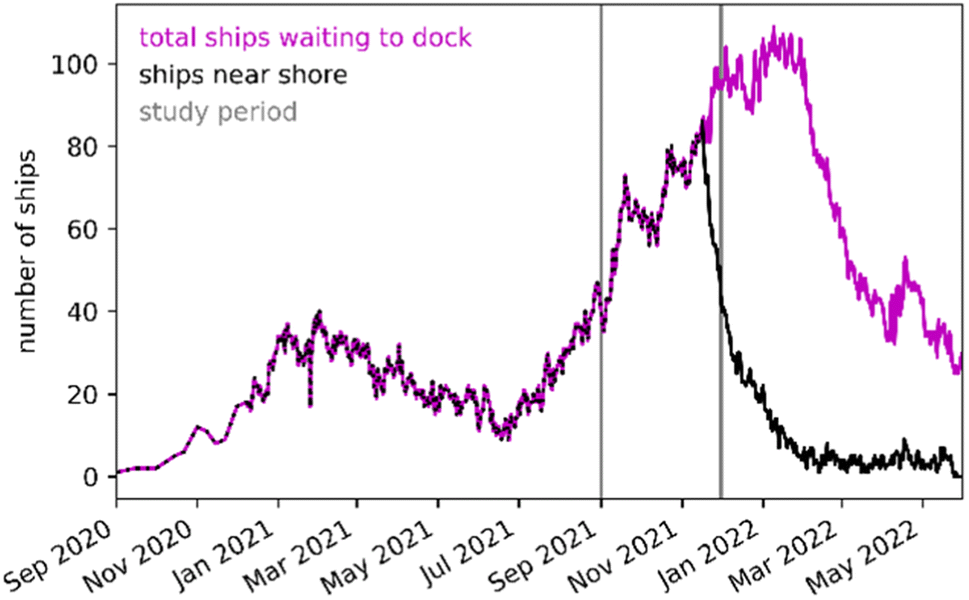
The ports of Los Angeles and Long Beach are adjoining seaports in Southern California which are the number one and two busiest ports in the United States (US).1 Previous work has shown that the ports and associated freight distribution have significant impacts on local air quality.2–5 Due to supply chain disruption resulting from the COVID-19 pandemic, the ports experienced a significant increase in cargo throughput in 2021. The combined throughput of twenty-foot equivalent units reached an all-time high (Fig. S1†), increasing by 16% in 2021 compared to the 2018–2019 average (Table S1†). The increased activity caused congestion at the ports, which led to many more cargo ships than normal waiting offshore for an opportunity to dock (Fig. 1). Ships were typically located near the California coast, using their auxiliary engines to provide power for shipboard functions. Many ships were waiting in waters immediately to the south of the ports and to the west of the coastline of Orange County (Fig. S2†).
 |
| | Fig. 1 Ships waiting to dock within 40 miles of the ports (black line) and the total number of ships waiting to dock (magenta line) at the ports of Los Angeles and Long Beach. During the study period of September–November 2021 (between the grey vertical lines), the number of ships near the ports reached its peak but began to decline after the ship queuing system was updated starting November 16, 2021. Data is from the Marine Exchange of Southern California viahttps://www.marketplace.org/2022/09/29/ship-backlog-at-southern-californias-ports-eases/. | |
The increase in ships and their proximity to the coast raised concerns about increased pollution in communities nearby. The California Air Resources Board (CARB) estimated that emissions of nitrogen oxides (NOx) and particulate matter (PM) from ships were 30 and 0.8 tons per day above business-as-usual conditions in November 2021.6 In addition to increased ship emissions, increased cargo throughput and congestion led to increased truck and rail traffic from the distribution of goods from the ports which further increased emissions nearby.7 According to emission inventory reports, diesel PM, NOx, and sulfur dioxide (SO2) emissions at the port of Los Angeles increased by 56%, 54%, and 145%, respectively, in 2021 compared to 2020.8 Emissions of these pollutants at the port of Long Beach also increased by 42%, 35%, and 38%, respectively, between 2020 and 2021.9 To alleviate the congestion, in October 2021 both ports and the Union Pacific Railroad Company shifted to 24/7 operation. In response to the excess ships anchored near the shore, an update to the system for ship queuing was implemented effective November 16, 2021. Under the new system, ships were required to wait approximately 150 miles away from the coast, whereas under the previous system, ships entered the queue once they came within 20 nautical miles of the ports.10
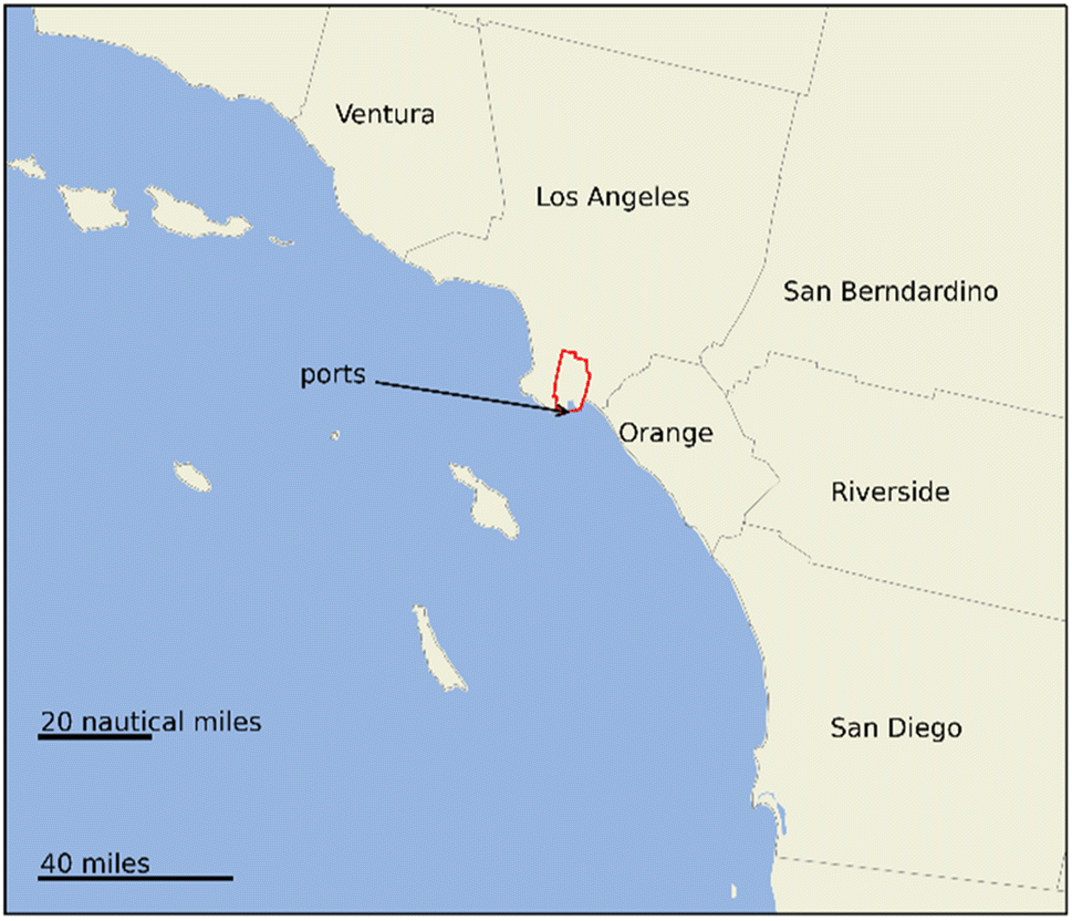
The new system reduced the number of ships near the coast (Fig. 1), but concerns remained about increased exposure to air pollution during this time. Some areas near the ports are already disproportionately impacted by pollution, raising additional concerns about the environmental justice implications of the additional air pollution exposure that may have resulted from the increase in port and associated goods movement activity. In particular, the communities of Wilmington, Carson, and West Long Beach, which are part of the Assembly Bill 617 (AB617)11 program established to monitor air pollution and reduce exposure in communities that are most heavily impacted by air pollution, are located near the ports (Fig. 2).
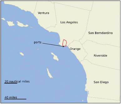 |
| | Fig. 2 Map of the study domain in Southern California. County names are indicated on the map. The arrow shows the location of the ports of Los Angeles and Long Beach. The red boundary shows the location of the Carson, Wilmington, and West Long Beach AB617 community defined by the CARB. Lines showing distances of 20 nautical miles and 40 miles which are referenced in the text are provided on the map for context. | |
Here, we use a combination of satellite-based observations, ground-based measurements, and chemical transport model (CTM) simulations to quantify changes in air pollution in Southern California during the period September–November 2021 when the number of ships waiting near the coast reached its peak (Fig. 1). A CTM can be used to estimate the impacts of changing emissions. However, the emissions inventories used as inputs to the CTM are uncertain, and accurately updating emissions to account for unexpected changes in source activity due to the COVID-19 pandemic and resulting disruptions in the global supply chain is challenging and adds even more uncertainty. Comparing observed changes in air quality across years can give some sense of the effects of changing emissions, but year-to-year variation in meteorological effects on air pollutant concentrations can make it difficult to attribute changes in air quality directly to changes in emissions. We examine the changes in nitrogen dioxide (NO2) and fine particulate matter (PM2.5) during this period. Satellite retrievals and surface observations are readily available for NO2, and NO2 provides a good indication of combustion emissions from ships. PM2.5 surface observations are also readily available, and PM2.5 is the air pollutant that most contributes to adverse health impacts.12 Effects of year-to-year differences in meteorology are estimated using a CTM. Observations are then adjusted for meteorological effects to obtain emission-related changes in 2021 compared to baseline levels in 2018 and 2019.
Methods and materials
Chemical transport model simulations
We use the Community Multiscale Air Quality (CMAQ) CTM version 5.3.3 (ref. 13) to perform the air quality simulations. The modeling domain is centered on Southern California with a horizontal resolution of 4 km (Fig. S3†). Simulations were performed for September–November (plus ten-day model spin-up over the last ten days of August to reduce the influence of initial conditions) for the years of 2018, 2019, and 2021 (B18, B19, and B21; B for base case). The average from 2018 and 2019 is used as the baseline with which to compare 2021. A simulation was not conducted for 2020 as the air quality during this year was significantly impacted by COVID-19 and thus does not provide a representative baseline since NO2 was below typical levels.14,15 Two additional simulations were conducted to estimate the influence of meteorology. These were performed using emissions for 2018 and 2019 as in the B18 and B19 simulations with meteorology from 2021 as in the B21 simulation (E18M21 and E19M21; E for emissions and M for meteorology). Lateral boundary conditions and initial conditions for the simulations were taken from daily average concentrations from a northern hemisphere CMAQ simulation conducted by US EPA as part of EPA's Air QUAlity TimE Series (EQUATES) project.16 Data from 2017 simulations were used as this was the most recent year that EQUATES results were available at the time the simulations were performed.
Emissions are based on the 2016 emissions modeling platform version 2 produced by US EPA and the emissions inventory collaborative.17 The platform uses a base year of 2016 and includes projected emissions for 2023. Emissions for 2018, 2019, and 2021 are obtained by linear interpolation of the emissions for each sector between the base 2016 emissions and the projected 2023 emissions. Details on each emissions sector and the projection methods used in the inventory are available in the platform technical support document.17 Fire emissions from the base inventory year of 2016 were used in all simulations so that the year-to-year changes in fire impacts did not obscure the effects of changes in anthropogenic emissions. We use seasonal average values to compare across years, so we expect that this averaging will reduce the influence of fires on the comparisons across years. Additionally, we expect that the incorporation of observations to apportion the changes to emissions and meteorology will capture any effects from differences in fires across years since fires will influence the observations which are used to derive the effects of emissions. Meteorological data for the CTM simulations are from the weather research and forecasting (WRF) model version 4.3.1.18 WRF data are prepared for the CMAQ simulations using the meteorology-chemistry interface processor19 version 5.1.
Satellite retrievals
TROPOspheric Monitoring Instrument (TROPOMI) follows a low-earth, sun-synchronous orbit with an equator overpass time of 13![[thin space (1/6-em)]](https://www.rsc.org/images/entities/char_2009.gif) :30 local solar time. Upgraded versions of the TROPOMI level 2 tropospheric NO2 product were released during the study period. Version 1.3 was in operation during September–November 2018–2019. Versions 2.2 and 2.3.1 were in operation during September–November 2021. The upgrades lead to increases in NO2 over cloud-free scenes, especially in polluted areas.20 To avoid an artificial positive jump in NO2, we use the product algorithm laboratory (PAL) dataset which was reprocessed with the version 2.3.1 algorithm.21 This dataset is available for May 1, 2018–November 14, 2021. We use the PAL data for September–November of 2018 and 2019 and for September 1–November 14, 2021. The version 2.3.1 product was used for November 15–30, 2021.
:30 local solar time. Upgraded versions of the TROPOMI level 2 tropospheric NO2 product were released during the study period. Version 1.3 was in operation during September–November 2018–2019. Versions 2.2 and 2.3.1 were in operation during September–November 2021. The upgrades lead to increases in NO2 over cloud-free scenes, especially in polluted areas.20 To avoid an artificial positive jump in NO2, we use the product algorithm laboratory (PAL) dataset which was reprocessed with the version 2.3.1 algorithm.21 This dataset is available for May 1, 2018–November 14, 2021. We use the PAL data for September–November of 2018 and 2019 and for September 1–November 14, 2021. The version 2.3.1 product was used for November 15–30, 2021.
Data is filtered to include only pixels with solar zenith angle less than 75, quality assurance flag value greater than 0.5, and cloud fraction less than 0.3. Like Cooper et al. (2020),22 we use the NO2 vertical profile from CMAQ with the TROPOMI averaging kernels to develop updated air mass factors (AMFs) to recalculate TROPOMI NO2 column totals. TROPOMI data are oversampled onto the 4 km × 4 km CMAQ model grid to facilitate comparisons between TROPOMI and CMAQ using an oversampling technique by Sun et al. (2018).23
Surface observations
Hourly NO2 surface observations were obtained from the CARB Air Quality and Meteorological Information System (https://www.arb.ca.gov/aqmis2/aqmis2.php). We use observations from 1 to 2 pm Pacific Standard Time to compare to the TROPOMI NO2 column totals since this includes the TROPOMI overpass time of 13:30 local solar time. We also compare TROPOMI NO2 to daily maximum surface NO2 as a sensitivity analysis. The comparison of surface observations and TROPOMI NO2 columns allows for evaluation of the suitability of TROPOMI to provide an indicator for changes in ground-level exposures. Near-road monitoring sites are excluded from this analysis. These sites are not suitable for comparison to TROPOMI because the typical sharp gradients in NO2 in the near-road environment cannot be resolved by TROPOMI. Exclusion of the near-road sites reduces the number of sites within the study domain from 44 to 39 sites. Daily average PM2.5 surface observations are obtained from the Air Quality System database (https://www.epa.gov/aqs). There are 45 PM2.5 sites within the study domain with data available for 2018, 2019, and 2021.
Traffic data
We use traffic volume data from the California Department of Transportation Performance Monitoring System (PeMS). Daily traffic volumes for September–November 2018, 2019, and 2021 for mainline highways were obtained from PeMS (https://pems.dot.ca.gov/). We calculate the change in traffic at each monitoring station as the total traffic volume in September–November 2021 compared to the average of the same period in 2018 and 2019. Data from individual stations are grouped by roadway and county, and the median change in traffic volume for stations along a particular roadway within a particular county is used to calculate the percent change in traffic along each section of roadway. We also obtained PeMS data for total vehicle miles traveled (VMT) and for truck VMT by roadway and county for the years of interest which were used to find the changes in total and truck VMT by county in 2021 compared to the baseline in 2018–2019.
Meteorological adjustments to observations
The differences between observations in 2018–2019 and 2021, whether satellite-based or ground-based, do not necessarily allow for the inference of the impacts of changing emissions. Part of the differences may be due to emissions, but some may be due to meteorology. We construct counterfactual meteorology CMAQ simulations by using emissions from 2018 (E18) or 2019 (E19) and meteorology from 2021 (M21) to construct two counterfactuals (E18M21; E19M21) to split TROPOMI NO2 columns and surface observations of NO2 and PM2.5 into meteorological and emission effects. The change in the observed value is separated into emissions and meteorological components using the effects of meteorology derived from the CMAQ simulations (eqn (1)–(5)). Here O represents the observed NO2 column total from TROPOMI or the observed surface NO2 or PM2.5 concentration, while M is the modeled value from CMAQ coincident with the 13:30 local solar time TROPOMI overpass for NO2 or the daily average modeled value for PM2.5.| |  | (1) |
| | | OE18M21,E19M21 = mean(O18,O19) × Mmet ratio | (2) |
| | | ΔO = ΔOemissions + ΔOmeteorology = O21 − mean(O18,O19) | (3) |
| | | ΔOemissions = O21 − OE18M21,E19M21 | (4) |
| | | ΔOmeteorology = ΔO − ΔOemissions | (5) |
Meteorological ratios (Mmet_ratio) are developed for both column total and surface level to separately account for meteorological effects throughout the entire vertical column and at the surface. A ratio method is used to represent the meteorological effects from CMAQ instead of an additive method that uses the modeled meteorological effect directly. One reason for this is that CMAQ column totals and surface concentrations of NO2 may differ from the observed levels, so it is more reasonable to use the CMAQ meteorological impacts in a relative sense instead of an absolute sense. A second reason is that an additive method can result in negative meteorologically adjusted column totals or surface observations which is avoided with the ratio method. While not identical to the method shown here, others have incorporated meteorological effects from CTMs with satellite data to estimate the effects of emission changes (e.g., Goldberg et al. (2020),14 Cao et al. (2022)24). Within the study domain, the CMAQ meteorology ratio (Mmet ratio from eqn (1)) for the NO2 vertical column totals has an average value of 1.0 and ranges from 0.7 to 1.5 (Fig. S4†).
Results and discussion
Model performance
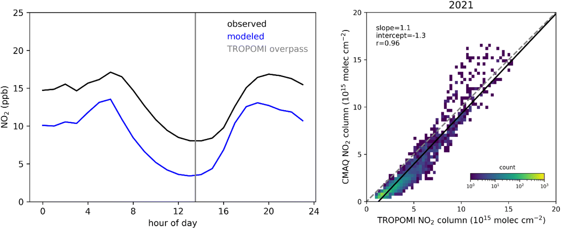
The performance of simulated NO2 is evaluated by comparison against surface monitors and TROPOMI vertical column densities (Fig. 3). Surface NO2 is biased low on average across all hours of the day, but CMAQ does reproduce the diurnal pattern of observed NO2. The seasonal average (September–November) column NO2 is also mostly biased low. The exception is in areas where modeled column NO2 is highest where the modeled column NO2 tends to be biased high which is consistent with other recent modeling studies.25–27 The spatial variability of TROPOMI is well captured by CMAQ as indicated by the slope and correlation very close to 1 (r = 0.96; slope = 1.1 for 2021). Performance is similar for all simulation years for both surface and column NO2 (Fig. S5†). Simulated meteorological values are evaluated against surface meteorological monitoring sites (Table S2†). For each meteorological parameter (relative humidity, temperature, and wind speed), CMAQ reproduces the observed diurnal variability (Fig. S6†). Wind speed has a normalized mean bias (NMB) of 47% to 49% across simulation years. Temperature is well simulated by the model but has a high bias (NMB = 7% to 8%). Relative humidity is biased low (NMB = −14% to −18%).
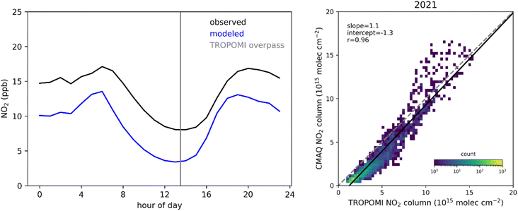 |
| | Fig. 3 Performance of CMAQ-simulated NO2 in September–November 2021 compared to surface observations (left) and TROPOMI vertical column densities (right). For the surface monitoring sites, observed and modeled NO2 are aggregated by hour across all sites in the CMAQ modeling domain. The TROPOMI overpass time of 13:30 local time is indicated with a grey vertical line. The comparison of vertical columns is for the average vertical column over the September–November study period. A one-to-one line is shown as a dashed grey line, and the linear regression between TROPOMI and CMAQ vertical columns is shown as a solid black line. The color scale represents the count of CMAQ/TROPOMI paired values that fall within each bin. | |
TROPOMI results and meteorological adjustments
TROPOMI NO2 columns decreased over Central Los Angeles (−10% on average) and in some offshore areas. After accounting for meteorological effects, these reductions were found to be largely driven by changing emissions (Fig. 4). Emission-related increases in NO2 were found over Tijuana, Mexico, near the southern edge of the study domain. In most other areas, column NO2 increased. The largest increases were seen in parts of Los Angeles and Orange Counties in areas directly east of the ports and east of the area where ships were waiting offshore (+28% on average). After accounting for meteorological effects, these areas were found to be significantly impacted by emissions. We conclude that these areas were impacted by increased port activity. This is based on inference due to the vicinity to the ports and the area where ships were waiting offshore, the finding that the changes are due to emissions rather than meteorology, and that the prevailing wind from west to east would transport emissions from the ports towards these areas (Fig. S7†). The changes in total and emission-related NO2 over Central Los Angeles and east of the ports were found to be statistically significant (Fig. S8†).
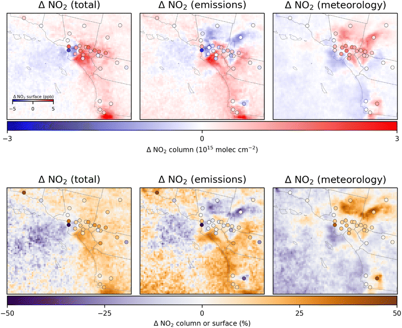 |
| | Fig. 4 Total change (left) in TROPOMI NO2 column in September–November 2021 compared to the average over the same period in 2018 and 2019. Total changes are apportioned to emissions (middle) and meteorology (right) using meteorological effects derived from CMAQ simulations. Circles show the analogous changes for 1–2 pm observations at NO2 surface monitoring sites. The inset color scale in the top left panel refers to the changes in surface observations (i.e., circle markers on the map) while the larger color scale below the top row of panels refers to the changes in vertical column densities. Both absolute changes (top row) and percent changes (bottom row) are shown. | |
Meteorology can impact NO2 columns due to differences from year to year in how pollutants are transported. In some areas, the meteorological impacts showed that increases in NO2 were solely due to meteorology. The portion of NO2 column changes resulting from emissions decreased in northern Los Angeles County and in parts of western Riverside and San Bernardino Counties (−17% in both areas). However, increases in NO2 because of meteorology (+25% in both areas) outweighed the emission-related reductions. In these areas, the changes in emission-related and meteorology-related changes were found to be statistically significant (Fig. S8†). Despite reductions in emission-related NO2 in parts of the counties, emission-related NO2 increased throughout most of San Bernardino and Riverside Counties, though these increases were mostly statistically insignificant. In general, meteorology in 2021 (compared to 2018 and 2019) tended to decrease NO2 in offshore areas and along the coast and tended to increase NO2 inland.
Surface vs. column NO2 changes
The change in 1–2 pm surface observations mostly agreed in direction with the changes derived from TROPOMI (Fig. 4 and S9†). The same was true for the emissions and meteorology influenced changes. The change in daily maximum surface NO2 agreed in direction with the change in TROPOMI columns for only about half of observation sites analyzed (Fig. S10†). Changes in TROPOMI NO2 columns may be a relevant indicator of changes in human exposures at the surface, but the once-per-day frequency of TROPOMI is a potential limitation. The surface NO2 sites closest to the ports showed small decreases in emission influenced NO2 while NO2 column totals showed increases in emission influenced NO2 in the same areas. This is explained by decreases in ground level local sources (e.g., traffic) near these sites offsetting increases in NO2 from ships that have a higher effective stack height and time to more fully diffuse vertically such that they had a smaller impact on inland ground-level sites while increasing the NO2 vertical column total.
PM2.5 changes
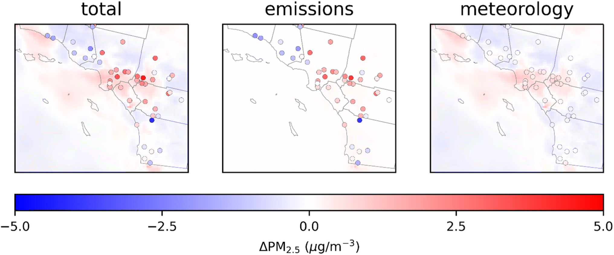
The changes in PM2.5 in the CMAQ simulations are almost entirely from the effects of meteorology (Fig. 5). The only changes in emissions included in the simulations are those that were projected based on the emissions inventory which does not account for the unexpected changes in emissions related to the port supply chain disruptions. The effects of meteorology on the changes in observed PM2.5 were small compared to the total change. The average meteorology ratio used to adjust observations only varied from 0.9 to 1.1 over the study domain (Fig. S11†). Observed PM2.5 was higher in September–November 2021 compared to the baseline of 2018–2019 at nearly all sites in Los Angeles, San Bernardino, Riverside, and Orange Counties. Changes in PM2.5 were mostly attributed to emissions rather than meteorology. PM2.5 increased on average across all sites by 0.7 μg m−3 and ranged from −4.1 μg m−3 to +4.5 μg m−3. The sites closest to the ports did have increased PM2.5 attributed to emissions, but these were not the sites with the largest increases in PM2.5 within the area.
 |
| | Fig. 5 Total change (left) in CMAQ-simulated average PM2.5 concentration in September–November 2021 compared to the average over the same period in 2018 and 2019. Total changes are apportioned to emissions (middle) and meteorology (right) using meteorological effects derived from CMAQ simulations. Circles show the analogous changes for PM2.5 observations. | |
We are not able to explicitly determine which sources of emissions may have contributed to the observed changes in PM2.5 concentrations. There are many different sources that could have had an effect, and the fact that much of PM2.5 is from secondary formation makes source attribution even more complicated. Notably, the site with the largest increase is in the city of Fontana in San Bernardino County in an area that has seen a significant increase in warehouses and distribution centers in recent years.28,29 Increased truck traffic near warehouses would be expected given the increase in port throughput during the study period. It is also possible that wildfires were a contributing factor as 2021 was a more active fire year (2.6 million acres burned across California) compared to 2018 (2.0 million acres burned) and 2019 (0.3 million acres burned) (https://www.fire.ca.gov/incidents). Speciated PM2.5 measurements from Chemical Speciation Network (CSN) observation sites in Central Los Angeles and western Riverside County showed elevated concentrations of nitrate (a secondary PM2.5 species formed from NO2) during high PM2.5 episodes in November 2021 (Fig. S12†), suggesting that increased NOx contributed to the increased PM2.5 observed during the study period.
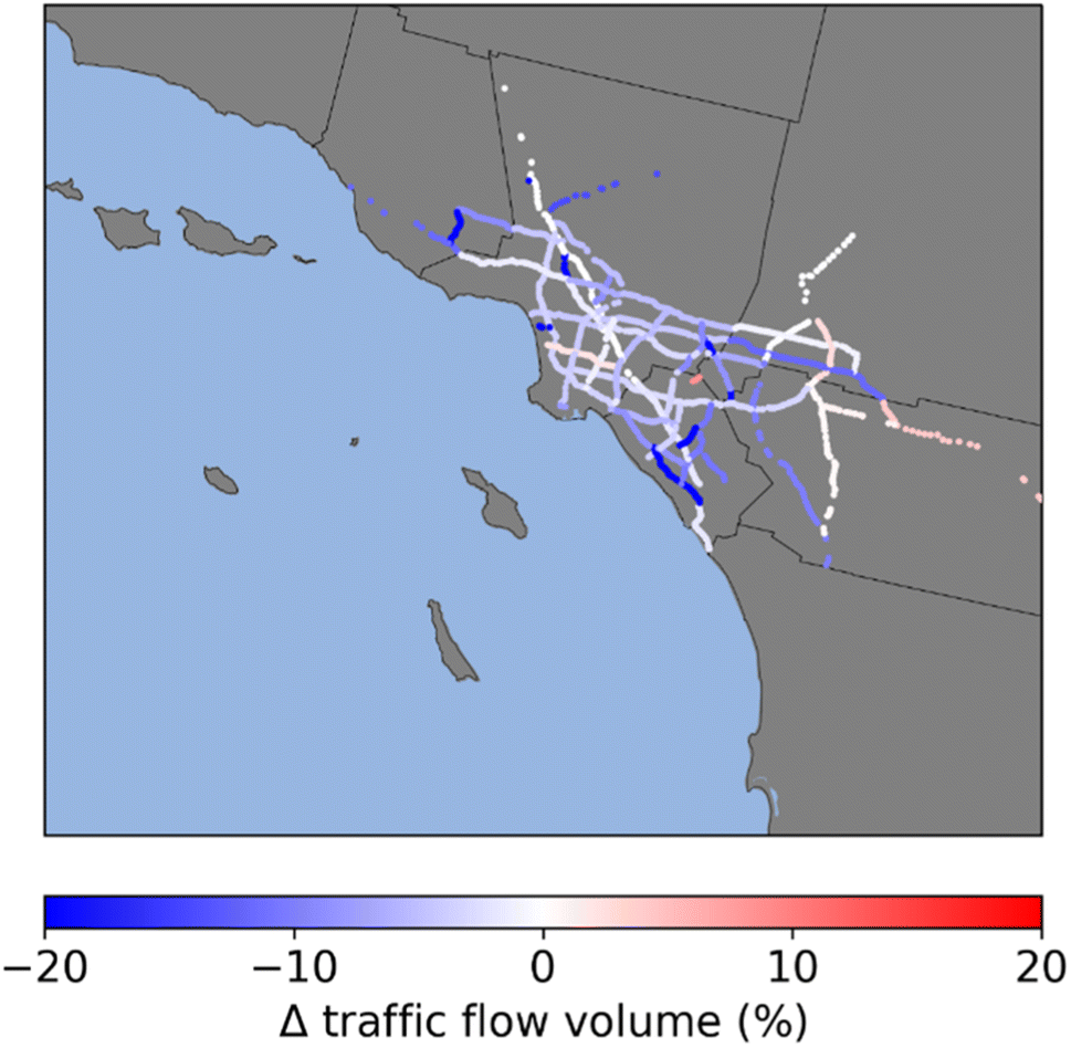
Relationship to traffic data
Some areas where emissions-related column NO2 decreased are near major highways (Fig. S14†). These areas include parts of Los Angeles, San Bernardino, and Riverside Counties. On the other hand, areas in Orange County and in other parts of San Bernardino and Riverside Counties where emissions-related column NO2 increased are also coincident with major highways. Using traffic flow volume PeMS data, we find that the relationship between changes in traffic flow volume and changes in the TROPOMI NO2 is mixed (Fig. 6). Traffic was overall lower in September–November 2021 compared to 2018–2019 except for a few roadways. In Central Los Angeles there was a decrease in traffic flow with corresponding reductions in total and emission-related TROPOMI NO2, particularly along the I110 freeway. Most other areas do not show a significant relationship between TROPOMI NO2 columns and total traffic flow. There were increases observed in truck VMT in Orange and San Bernardino Counties despite decreases in total VMT (Fig. S15†) during the same period which could have contributed to increases in NO2 and PM2.5 seen in those areas.
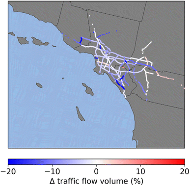 |
| | Fig. 6 Percent change in total traffic flow volume at Caltrans Performance Monitoring System monitoring stations in September–November 2021 compared to the average over the same time in 2018 and 2019. Traffic data from individual monitoring stations are grouped by county and roadway and shown as the median change in traffic flow for stations along each roadway within a particular county. | |
Conclusions
When analyzing the air quality impacts of short-term changes in emissions such as the congestion at the Ports of Los Angeles and Long Beach, direct comparisons of year-to-year changes in observations, whether satellite-based or ground-based, do not necessarily reflect changes due to emissions. Changes in meteorology across years can obscure the signal of emissions impacts. The method used here combines satellite-based and ground-based observations with CTM results to account for the meteorological effects. This allows for the apportionment of changes across years to emissions and meteorology separately based on changes in observations and CTM-simulated meteorological impacts. Some uncertainty in separating emissions and meteorology influences still remains. The meteorological impacts may be biased since they are derived from models. The CTM also may not accurately simulate the NO/NO2 split of total NOx which would affect the comparison of modeled NO2 to observed.
Despite the uncertainties, results suggest that there was an adverse impact on NO2 from increased ship and port activity. This was seen most predominantly in parts of Los Angeles and Orange Counties directly east of the ports and east of the offshore areas in which ships were waiting which is in the direction of the prevailing wind. Compared to prior years, there were also widespread increases in observed PM2.5 across much of the area which were attributed mostly to emissions. PM2.5 increased at the sites closest to the ports, but the largest increase in PM2.5 was found at a site in an area that has seen rapid growth in warehouses and distribution centers in recent years. Additional research relating to the health and environmental justice impacts of increased port activity in the Los Angeles area is warranted. In addition to direct emissions from ships and ports, potential increases in emissions from rail, trucking, and warehousing associated with increased goods throughput should be considered. Other ports also experienced increases in activity following the COVID-19 pandemic, and further investigation into the air quality effects of supply chain disruptions on ports around the US and globally would be helpful in determining if similar impacts on air quality were seen surrounding other ports or if this was isolated to only a few areas.
Author contributions
TNS: conceptualization, methodology, investigation, software, visualization, writing – original draft. JK: methodology, software, writing – review and editing, funding acquisition. MTO: writing – review and editing, funding acquisition. SH: investigation, visualization, writing – review and editing. AGR: conceptualization, methodology, investigation, resources, supervision, writing – review and editing, funding acquisition.
Conflicts of interest
There are no conflicts of interest.
Acknowledgements
Funding for this work was from NASA HAQAST (grant number 80NSSC21K0506) and from the Phillips 66 Company. The views expressed in this document are solely those of the authors and do not necessarily reflect those of the funding organizations, nor do the funders endorse any products or commercial services mentioned in this publication. The contributions SH are carried out at the Jet Propulsion Laboratory, California Institute of Technology, under contract with NASA.
References
-
World Shipping Council, The Top 50 Container Ports, 2022, https://www.worldshipping.org/top-50-ports, accessed October 25 2022 Search PubMed.
- K. H. Kozawa, S. A. Fruin and A. M. Winer, Near-road air pollution impacts of goods movement in communities adjacent to the Ports of Los Angeles and Long Beach, Atmos. Environ., 2009, 43, 2960–2970 CrossRef CAS.
- A. Cohan, J. Wu and D. Dabdub, High–resolution pollutant transport in the San Pedro Bay of California, Atmos. Pollut. Res., 2011, 2, 237–246 CrossRef CAS.
- A. Mousavi, M. H. Sowlat, S. Hasheminassab, O. Pikelnaya, A. Polidori, G. Ban-Weiss and C. Sioutas, Impact of particulate matter (PM) emissions from ships, locomotives, and freeways in the communities near the ports of Los Angeles (POLA) and Long Beach (POLB) on the air quality in the Los Angeles county, Atmos. Environ., 2018, 195, 159–169 CrossRef CAS.
- S. Vutukuru and D. Dabdub, Modeling the effects of ship emissions on coastal air quality: a case study of southern California, Atmos. Environ., 2008, 42, 3751–3764 CrossRef CAS.
-
California Air Resources Board, Emissions Impacts of Freight Movement Increases and Congestion near Ports of Los Angeles and Long Beach: June 2022, 2022, https://ww2.arb.ca.gov/sites/default/files/2022-06/SPBP_Freight_Congestion_Emissions_30JUN2022.pdf Search PubMed.
-
California Air Resources Board, Emissions Impact of Recent Congestion at California Ports: Quantifying Emissions Impacts of Freight Movement Increases and Congestion in Container Vessels, Locomotives, and Heavy-duty Trucks Near Major Seaports in California, 2021, https://ww2.arb.ca.gov/sites/default/files/2021-09/port_congestion_anchorage_locomotives_truck_emissions_final_%28002%29.pdf Search PubMed.
-
Port of Los Angeles, Inventory of Air Emissions 2021, Technical Report, 2022, https://kentico.portoflosangeles.org/getmedia/f26839cd-54cd-4da9-92b7-a34094ee75a8/2021_Air_Emissions_Inventory Search PubMed.
-
Port of Long Beach, Air Emissions Inventory – 2021, 2022, E-mail: https://polb.com/download/14/emissions-inventory/15418/2021-air-emissions-inventory.pdf Search PubMed.
-
Marine Exchange of Southern California, Container Vessel Queuing Process for the Ports of Los Angeles, Long Beach, and Oakland v.2, 2022 Search PubMed.
-
Nonvehicular Air Pollution: Criteria Air Pollutants and Toxic Air Contaminants, 2017, https://leginfo.legislature.ca.gov/faces/billTextClient.xhtml?bill_id=201720180AB617 Search PubMed.
-
GBD 2019 Risk Factors Collaborators, Global burden of 87 risk factors in 204 countries and territories, 1990-2019: a systematic analysis for the Global Burden of Disease Study 2019, Lancet, 2020, 396, 1223–1249 Search PubMed.
-
USEPA, CMAQ (5.3.3), Zenodo, 2021, DOI:10.5281/zenodo.5213949.
- D. L. Goldberg, S. C. Anenberg, D. Griffin, C. A. McLinden, Z. Lu and D. G. Streets, Disentangling the impact of the COVID-19 lockdowns on urban NO2 from natural variability, Geophys. Res. Lett., 2020, 47, e2020GL089269 CrossRef CAS PubMed.
- H. A. Parker, S. Hasheminassab, J. D. Crounse, C. M. Roehl and P. O. Wennberg, Impacts of traffic reductions associated with COVID-19 on Southern California air quality, Geophys. Res. Lett., 2020, 47, e2020GL090164 CrossRef CAS PubMed.
-
USEPA, EQUATESv1.0: Emissions, WRF/MCIP, CMAQv5.3.2 Data – 2002-2017 US_12km and NHEMI_108km, UNC Dataverse, V5, 2021 Search PubMed.
-
USEPA, Technical Support Document (TSD) Preperation of Emissions Inventories for the 2016v2, North American Emissions Modeling Platform, 2021 Search PubMed.
-
W. C. Skamarock, J. B. Klemp, J. Dudhia, D. O. Gill, Z. Liu, J. Berner, W. Wang, J. G. Powers, M. G. Duda, D. M. Barker and X.-Y. Huang, A Description of the Advanced Research WRF Version 4, NCAR Tech. Note NCAR/TN-556+STR, 2019, DOI:10.5065/1dfh-6p97.
- T. L. Otte and J. E. Pleim, The meteorology-chemistry interface processor (MCIP) for the CMAQ modeling system: updates through MCIPv3.4.1, Geosci. Model Dev., 2010, 3, 243–256 CrossRef.
- J. van Geffen, H. Eskes, S. Compernolle, G. Pinardi, T. Verhoelst, J. C. Lambert, M. Sneep, M. ter Linden, A. Ludewig, K. F. Boersma and J. P. Veefkind, Sentinel-5P TROPOMI NO2 retrieval: impact of version v2.2 improvements and comparisons with OMI and ground-based data, Atmos. Meas. Tech., 2022, 15, 2037–2060 CrossRef CAS.
-
J. H. G. M. van Geffen, H. J. Eskes, K. F. Boersma and J. P. Veefkind, TROPOMI ATBD of the Total and Tropospheric NO2 Data Products, 2022 Search PubMed.
- M. J. Cooper, R. V. Martin, D. K. Henze and D. B. A. Jones, Effects of a priori profile shape assumptions on comparisons between satellite NO2 columns and model simulations, Atmos. Chem. Phys., 2020, 20, 7231–7241 CrossRef CAS.
- K. Sun, L. Zhu, K. Cady-Pereira, C. Chan Miller, K. Chance, L. Clarisse, P. F. Coheur, G. González Abad, G. Huang, X. Liu, M. Van Damme, K. Yang and M. Zondlo, A physics-based approach to oversample multi-satellite, multispecies observations to a common grid, Atmos. Meas. Tech., 2018, 11, 6679–6701 CrossRef.
- H. Cao, D. K. Henze, K. Cady-Pereira, B. C. McDonald, C. Harkins, K. Sun, K. W. Bowman, T.-M. Fu and M. O. Nawaz, COVID-19 lockdowns afford the first satellite-based confirmation that vehicles are an under-recognized source of urban NH3 pollution in Los Angeles, Environ. Sci. Technol. Lett., 2022, 9, 3–9 CrossRef CAS.
- M. Li, B. C. McDonald, S. A. McKeen, H. Eskes, P. Levelt, C. Francoeur, C. Harkins, J. He, M. Barth, D. K. Henze, M. M. Bela, M. Trainer, J. A. de Gouw and G. J. Frost, Assessment of updated fuel-based emissions inventories over the contiguous United States using TROPOMI NO2 retrievals, J. Geophys. Res.: Atmos., 2021, 126, e2021JD035484 CrossRef CAS.
- D. L. Goldberg, M. Harkey, B. de Foy, L. Judd, J. Johnson, G. Yarwood and T. Holloway, Evaluating NOx emissions and their effect on O3 production in Texas using TROPOMI NO2 and HCHO, Atmos. Chem. Phys., 2022, 22, 10875–10900 CrossRef CAS.
- A. S. Lawal, A. G. Russell and J. Kaiser, Assessment of airport-related emissions and their impact on air quality in Atlanta, GA, using CMAQ and TROPOMI, Environ. Sci. Technol., 2022, 56, 98–108 CrossRef CAS PubMed.
- P. N. deSouza, S. Ballare and D. A. Niemeier, The environmental and traffic impacts of warehouses in southern California, J. Transport Geogr., 2022, 104, 103440 CrossRef.
- Q. Yuan, Mega freight generators in my backyard: a longitudinal study of environmental justice in warehousing location, Land Use Policy, 2018, 76, 130–143 CrossRef.
|
| This journal is © The Royal Society of Chemistry 2024 |
Click here to see how this site uses Cookies. View our privacy policy here. 
 Open Access Article
 This Open Access Article is licensed under a Creative Commons Attribution-Non Commercial 3.0 Unported Licence
 a,
Jennifer
Kaiser
ab,
M. Talat
Odman
a,
Jennifer
Kaiser
ab,
M. Talat
Odman