
 Open Access Article
 This Open Access Article is licensed under a Creative Commons Attribution-Non Commercial 3.0 Unported Licence
Multi-task scattering-model classification and parameter regression of nanostructures from small-angle scattering data†
Batuhan
Yildirim
 abc,
James
Doutch
b and
Jacqueline M.
Cole
*abc
abc,
James
Doutch
b and
Jacqueline M.
Cole
*abc
aCavendish Laboratory, Department of Physics, University of Cambridge, J.J. Thomson Avenue, Cambridge, CB3 0HE, UK. E-mail: jmc61@cam.ac.uk
bISIS Neutron and Muon Source, STFC Rutherford Appleton Laboratory, Didcot, Oxfordshire, OX11 0QX, UK
cResearch Complex at Harwell, Rutherford Appleton Laboratory, Didcot, Oxfordshire, OX11 0FA, UK
First published on 12th March 2024
Abstract
Machine learning (ML) can be employed at the data-analysis stage of small-angle scattering (SAS) experiments. This could assist in the characterization of nanomaterials and biological samples by providing accurate data-driven predictions of their structural parameters (e.g. particle shape and size) directly from their SAS profiles. However, the unique nature of SAS data presents several challenges to such a goal. For instance, one would need to develop a means of specifying an input representation and ML model that are suitable for processing SAS data. Furthermore, the lack of large open datasets for training such models is a significant barrier. We demonstrate an end-to-end multi-task system for jointly classifying SAS data into scattering-model classes and predicting their parameters. We suggest a scale-invariant representation for SAS intensities that makes the system robust to the units of the input and arbitrary unknown scaling factors, and compare this empirically to two other input representations. To address the lack of available experimental datasets, we create and train our proposed model on 1.1 million theoretical SAS intensities which we make publicly available. These span 55 scattering-model classes with a total of 219 structural parameters. Finally, we discuss applications, limitations and the potential for such a model to be integrated into SAS-data-analysis software.
1 Introduction
Small-angle scattering (SAS) (of X-rays, neutrons or optical light)1–4 are widely used experimental procedures for probing the nanostructure of materials, polymers, proteins and other biological matter. Relationships between observable experimental scattering intensities and the morphology of the scatterers can be exploited to shed light on the underlying structure of a sample, including the structure of individual scatterers as well as their inter-particle distance distribution functions. Following the acquisition of SAS data from a sample, data analysis is generally carried out in software such as SasView (http://www.sasview.org/), in which a library of many possible scattering models are available. Scattering models are analytical expressions that result from integrating the scattering density of a shape over 3-D space (see Fig. 1 for an example). These expressions can have many structural parameters that influence the profile of the resulting SAS intensity. The goal of SAS-data analysis is typically to determine these unknown parameters using least-squares fitting of theoretical models to experimental data. Predictive analytics deployed at the data-analysis stage of SAS experiments could assist researchers in characterizing their samples by providing accurate estimates of model-function classes to try, as well as estimates of morphological parameters. Such tools may speed up analysis of SAS data by nudging experts in the right direction and removing some guess work from the procedure.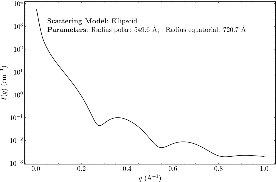 | ||
| Fig. 1 An example of an idealized scattering model and the scattering intensity, I(q), it produces. This particular model represents the scattering from an ellipse with polar and equatorial radii of 549.6 and 720.7 Å respectively. In this case, the scattering intensity is a function of q and the radii parameters that are specific to ellipsoids. | ||
Machine-learning (ML) models that take as input SAS intensities and estimate scattering-model classes and their parameters have the potential to be integrated into SAS-data analysis software, although there are several challenges that must first be addressed. The lack of large sets of experimental data labeled with scattering-model classes and their parameters means that such models must be trained on synthetic data, which raises questions of generalizability. Additionally, SAS intensities in their raw form are not particularly suitable as inputs to ML models. They can span several orders of magnitude in intensity and have arbitrary scale factors and additive background shifts that make it difficult to attribute a single SAS intensity to a particular scattering-model class and set of parameters. For such a system to be practically useful as a data-analysis tool, uncertainty quantification is likely to be an important feature. In cases where the input experimental data are noisy, or when the data result from a structure with a scattering-model class that is unknown to the ML model, we should expect high uncertainty values. This will allow sensible conclusions to be drawn in the cases where input experimental data are out-of-distribution relative to the training data. Small-angle neutron scattering (SANS) data pose additional challenges as instrumental resolution functions (i.e., smearing parameters), that are unique to individual SANS instruments, can cause variability in data resulting from the same sample measured using different SANS instruments.
We endeavor to address some of these challenges in this work. Thereby, we create the SAS-55M-20k dataset, consisting of 1.1 million theoretical 1-D SAS intensities with corresponding discrete scattering-model classes and their continuous parameters.5 This dataset is made publicly available alongside this paper, including the training and test splits to ease benchmarking of any future models trained on this dataset. Full details on the construction and composition of the dataset can be found in the ESI.† We propose a simple scale invariant representation of SAS intensities that is suitable for input to ML algorithms, and empirically compare this to two other scale invariant representations (including one which is commonly used in the literature). Primarily, we present a multi-task transformer neural network that takes as input a 1-D SAS intensity and jointly estimates the scattering-model class that produced it (classification), as well as the continuous parameters of the scattering model (regression), and evaluate its performance on both tasks. Finally, we discuss some limitations and propose ways in which the data and model may be improved to be more applicable to real 1-D SAS data.
1.1 Related work
Recently, there have been many studies that apply ML to 1-D X-ray and neutron scattering data to predict structural parameters and properties of a variety of organic and inorganic structures.6–20 We briefly highlight the few that are most relevant to our work. Franke et al. developed a ML technique to analyze SAXS data, categorizing biomolecules into distinct shapes and estimating their structural parameters.6 They first assembled and normalized a dataset consisting of ideal SAXS signals of biological macromolecules, which they further represented in a three-dimensional feature space where each feature is a Porod invariant calculated with differing parameters. The authors fit two k-nearest neighbors (kNN) models to this data for shape classification and structural parameter estimation. Molodenskiy et al. employed a simple multi-layer perceptron with a single hidden layer to predict molecular weights (MW) and maximum intra-particle distances of nucleic acids and folded/intrinsically disordered proteins from small-angle X-ray scattering (SAXS) data.8 They simulated SAXS data from experimentally determined protein structures21 and used this to train and evaluate their models. They showed that their model was able to predict MW with smaller errors than several analytical methods while relying on fewer assumptions in comparison. This work shows that neural networks can be employed to accurately estimate structural parameters from SAS data, and hints at their potential to be integrated into SAS-data-analysis toolkits for fast and reliable analysis. Butler et al. applied convolutional neural networks to inelastic neutron scattering data to discriminate between magnetic phases of half-doped magnetites.22 Since their model was trained on synthetic data, they integrated uncertainty quantification into their method such that when applied to real experimental data, the reliability of predictions can be assessed. Most relevant to our work are the methods developed by Archibald et al.7 They applied ML methods, namely weighted kNN and Gaussian processes, to classify SAS data into several scattering-model classes that are available in the SasView package. Given input SAS data and a predicted model class, they used a stochastic gradient-descent fitting procedure to obtain the parameters of the model class that produced the input data. Lutz-Bueno et al. introduce a model-free classification method for small-angle and wide-angle X-ray scattering signals, where they use only the inflection points of a signal as features for a clustering and segmentation model.19 By using only the inflection points as features for their model, they reduce the dimensionality of the input data significantly and simplify the analysis of large datasets as demonstrated through applications in segmenting mudrock and tissue samples. Finally, in a novel approach to SAS analysis, Heil et al. present a method that concurrently determines the form and structure factors in dense macromolecular solutions.23 Termed CREASE, this method employs a genetic algorithm to transform SAS intensity data into a real-space particle configuration. Form and structure factors are derived from this configuration using either the Debye scattering equation or an auxiliary machine learning model. The efficacy of CREASE is underscored by its ability to produce form and structure factors that more accurately align with target scattering profiles than traditional analytical methods.2 Results and discussion
2.1 Dataset construction and composition
The data used in this work were generated with SasView and the sasmodels package (version 0.96) using open-source code written by Archibald et al.7 We used 55 of the 73 scattering-model classes that are available in SasView to generate 20![[thin space (1/6-em)]](https://www.rsc.org/images/entities/char_2009.gif) 000 idealized SAS intensity functions of dilute (i.e., structure factor S(q) = 1) systems from each class with parameters sampled randomly in each case. We have ensured that general parameters common to all model classes, including polydispersity and scattering length densities for solvents and model-specific features, were randomly sampled for each instance in our dataset. This effectively ensures that models trained on this data, including ours, are robust to varying ranges of polydispersities and contrasts. In each case, the scattering intensities were generated with fixed volume fractions (i.e., sample concentrations) and background constants (full details on how parameters were sampled can be found in Archibald et al.7). The total number of scattering-model parameters across all 55 classes is 219. Some model classes were excluded because they were computationally infeasible (i.e., too slow) to compute or caused out-of-memory errors. The resulting dataset comprised 1.1 million samples, which we split into training and test data using a 80:20 split. We call this the SAS-55M-20k dataset, and we provide both training and test sets through this publication to facilitate further work on applying ML and other computational methods to 1-D SAS intensities with known parameters. Details on how to download the SAS-55M-20k dataset5 can be found at https://github.com/by256/sasformer.
000 idealized SAS intensity functions of dilute (i.e., structure factor S(q) = 1) systems from each class with parameters sampled randomly in each case. We have ensured that general parameters common to all model classes, including polydispersity and scattering length densities for solvents and model-specific features, were randomly sampled for each instance in our dataset. This effectively ensures that models trained on this data, including ours, are robust to varying ranges of polydispersities and contrasts. In each case, the scattering intensities were generated with fixed volume fractions (i.e., sample concentrations) and background constants (full details on how parameters were sampled can be found in Archibald et al.7). The total number of scattering-model parameters across all 55 classes is 219. Some model classes were excluded because they were computationally infeasible (i.e., too slow) to compute or caused out-of-memory errors. The resulting dataset comprised 1.1 million samples, which we split into training and test data using a 80:20 split. We call this the SAS-55M-20k dataset, and we provide both training and test sets through this publication to facilitate further work on applying ML and other computational methods to 1-D SAS intensities with known parameters. Details on how to download the SAS-55M-20k dataset5 can be found at https://github.com/by256/sasformer.
2.2 Input representation
A SAS intensity function, I(q), refers to the intensity of the scattered neutron/X-ray beam as a function of the magnitude of the scattering vector q = 4πsin(θ)/λ, where θ is the half-angle between the incident beam and a detector. Using raw I(q) data as input to neural networks presents some challenges. SAS intensities can span several orders of magnitude in scale, while neural networks typically work best with standardized inputs that have zero mean and unit variance. Moreover, the scale of I(q) depends on arbitrary scaling factors that result from experimental or sample conditions as well as the units used to describe the function. Consequently, although a structural system may be characterized by a single model function specified by a particular set of parameters, various scale factors and units can afford a potentially large number of I(q) functions that could describe the same system. Thus, a scale invariant input representation is required.
To achieve scale invariance, we apply what we call a “quotient transform” to I(q). If I(qn) and I(qn+1) are the scattering intensities at indices n and n + 1 of a discretized I(q) function, the quotient transform is 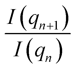 . By applying this transformation, any scale factors (such as those occurring from sample concentrations) are cancelled as can be seen by considering if sI(q) is a scattered intensity scaled by an arbitrary scale factor, s, then the quotient transform of sI(q) is
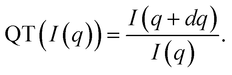
 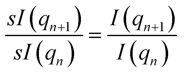 . Formally, the quotient transform of I(q) is expressed as:
 | (1) |
In practice, we take the logarithm of the quotient transform to reduce the variability between classes of scattering-model functions that are present in the data. This can be interpreted as a difference transform in log-space since 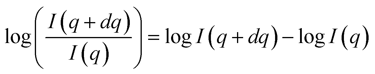 . Examples of SAS intensities and their log-quotient transforms are shown in Fig. 2.
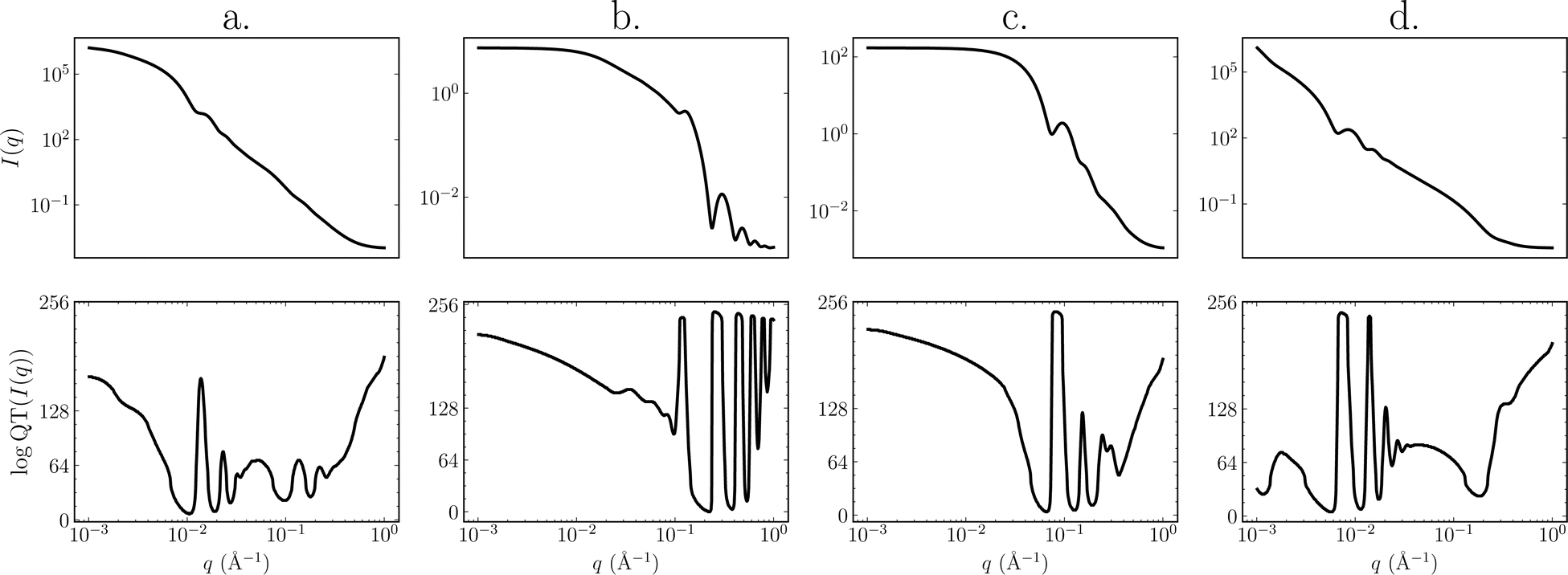 | ||
| Fig. 2 Illustration showing log-scaled I(q) samples from the SAS-55M-20k dataset (top row) and their discretized log quotient transformed versions (bottom row). The y-axes in the bottom row represent the bin of the value after discretization. The x-axes in both rows range from 0.001 to 1.0 Å−1. The quotient transform appears to exaggerate minor features in I(q). (a) Core shell ellipsoid model (equatorial radius of core – 285.833 Å; shell thickness at equator – 75.221 Å; axial ratio of core – 4.956 Å; ratio of thickness of shell at pole and equator – 9.349). (b) Linear pearls model (radius – 19.165 Å; length of string segment – 13.311 Å; number of pearls – 5). (c) Fractal core–shell model (fractal dimension – 2; radius – 28.511 Å; volume fraction – 0.041; shell thickness – 27.699 Å; correlation length – 116.349 Å). (d) Lamellar stack paracrystal model (lamellar spacing – 8.691 Å; sheet thickness – 26.484 Å; number of layers – 116). | ||
Besides enabling inputs to be tokenized, discretizing the input has two other notable benefits. Firstly, by forcing the input values into a set number of bins, small fluctuations in the input are eliminated, increasing the signal-to-noise ratio. This can be particularly useful for experimental SAS data which tend to be noisy. The second benefit is that discretizing the input makes any subsequent ML model trained on these inputs somewhat robust to background shifts that are commonly present in experimentally obtained SAS data. These additive background constants are often observed to be in the range of 0.001 to 0.01 and the discretizing process neutralizes them since they are so small relative to the range of values that is spanned by SAS data, particularly at lower q values. In our method, quotient transformed data are discretized using an ordinal encoding scheme and a quantile-based binning strategy. The ordinal encoding scheme transforms continuous input values into discrete bins represented by integer values, where each bin corresponds to a specific range of the continuous input. The quantile-based binning strategy ensures that an equal number of data points are in each bin. This is particularly useful for handling skewed distributions, which some portions SAS intensities can be when compared across scattering models and across the entire dataset.
2.3 SAS transformer
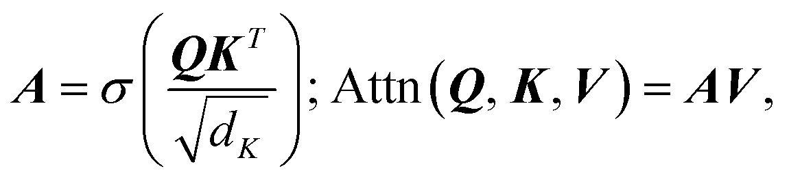
A neural network was chosen for this problem as these types of ML models can be flexibly constructed to create architectures with multiple inputs and outputs, while most other ML models can not. The problem of predicting a scattering-model class and its parameters is multi-task in nature, so we employed an encoder-decoder architecture with two decoders: one for scattering-model class classification and one for scattering-model parameter regression. Besides being state of the art for sequence modeling,27–30 the fact that transformers support masked inputs make them particularly suitable for SAS data modeling. The q values spanned by experimental SAS data depend on experimental setup choices and instrumental limitations such as the size of the detector surface, size of the direct beam stop, detector pixel size, beam wavelength, etc. Thus we expect to see a variety of q-ranges in real experimental SAS data. During training of our model which is trained on synthetic data with a fixed q-range of [0.001, 1.0] Å−1, we can mask inputs beyond a randomly selected q value (e.g., 0.5 Å−1) since batches of data are sampled at each training step, making the model robust to inputs with different q-ranges. If the trained model is subsequently used for prediction on real SAS data, one can simply append dummy I(q) values until the q-range of the input data matches that of the training data, and mask these values such that the model does not consider them during processing.We now provide a high level overview of transformers and attention in the context of our model's architecture, but we refer the reader to Vaswani et al.24 and Jeagle et al.26 for full details on attention and Perceiver IO, respectively. The SASformer architecture (Fig. 3) consists of (a) an encoder that maps inputs to a space with a smaller number of latent feature vectors for efficient processing; (b) two decoders – one for classifying the scattering-model function and another for predicting the functional parameters of the scattering model. The main component of both the encoder and decoders is the attention mechanism,
 | (2) |
| K = XWK; V = XWV; | (3) |
 | (4) |
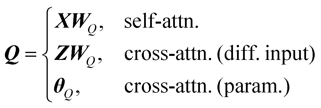
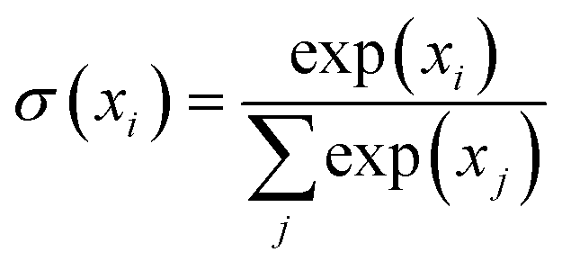 is the softmax function and dK is the feature dimensionality of K. Q, K and V are queries, keys and values, respectively, which can vary depending on whether self-attention or cross-attention is being performed on the inputs (eqn (2) and (3)). The former entails linear projections of the input array by a parameter matrix, hence the name ‘self’-attention, since queries, keys and values are all computed from the same input. The latter involves keys and values that are computed from the input array, while the query is either computed from a distinct and separate input (Z in case 2, eqn (2)) or it can be a learnable parameter matrix (θQ in case 3, eqn (2)); thus it is known as cross-attention. Following Perceiver IO, the SASformer architecture employs self-attention and cross-attention with parameter-only queries at various stages.
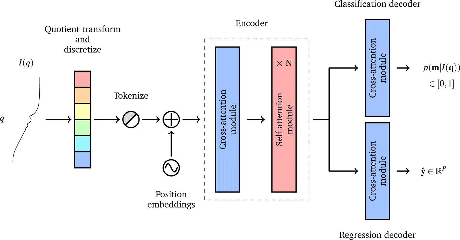 | ||
Fig. 3 Data pre-processing steps and SASformer model overview. The input is a quotient transformed and discretized I(q), which is tokenized and position encoded resulting in a matrix X ∈ ![[Doublestruck R]](https://www.rsc.org/images/entities/char_e175.gif) S×F, where S and F are the sequence and feature dimensionalities, respectively. A cross-attention layer then transforms this to a latent representation Z ∈ T×F with a smaller sequence dimension (T < S) for efficient processing by N subsequent self-attention blocks. The latent representation is then passed through two decoders (that are single cross-attention blocks), one that outputs a probability distribution over all scattering-model classes m and another that outputs a P-dimensional vector of continuous parameters for all scattering-model classes. Using an efficient variant of the transformer24 architecture called Perceiver IO,25,26 we developed a neural network to characterize small-angle scattering data into a scattering-model class and its parameters. We call our model SASformer. S×F, where S and F are the sequence and feature dimensionalities, respectively. A cross-attention layer then transforms this to a latent representation Z ∈ T×F with a smaller sequence dimension (T < S) for efficient processing by N subsequent self-attention blocks. The latent representation is then passed through two decoders (that are single cross-attention blocks), one that outputs a probability distribution over all scattering-model classes m and another that outputs a P-dimensional vector of continuous parameters for all scattering-model classes. Using an efficient variant of the transformer24 architecture called Perceiver IO,25,26 we developed a neural network to characterize small-angle scattering data into a scattering-model class and its parameters. We call our model SASformer. | ||
2.4 Scattering-model classification
To assess how well SASformer can correctly classify SAS intensities into scattering-model classes, we used accuracy and top-3 accuracy as our primary metrics. Top-3 accuracy can be calculated since the classification output of the model is a probability distribution over all scattering-model classes. In calculating top-3 accuracy, we label an output as correctly classified if the top-3 output probability estimates contains the ground-truth scattering-model class for an input instance. Since the test dataset we used is considered balanced, as there are exactly 4000 instances of each scattering-model class, it was not necessary to use precision and recall to evaluate classification performance. As a baseline for the classification task, we used k-nearest neighbors (kNN) with k = 5 to predict the scattering model class of each instance in the test set. The kNN classifier was trained on the same training set as SASformer and tested on the same test set. The baseline model achieved an average accuracy and average top-3 accuracy of 0.713 and 0.857, respectively. The full results of the baseline model's classification performance on each individual model class are presented in the ESI.†Averaged over all scattering-model classes, accuracy and top-3 accuracy are 0.95674 and 0.99257, respectively. If such a model is incorporated into SAS-data-analysis software, the exceptional top-3 accuracy suggests that proposing the 3 most probable scattering models is likely to be more informative to a user, since the top-3 classification predictions almost always contain the true scattering-model class. Inter-scattering model-classification results are presented in Table 1, where the values of the metrics make it clear that some scattering models are more difficult to predict than others. We observed that most of the errors result from misclassifying a scattering-model as a different but similar model from the same family – a group of related scattering-model classes. For example, when the input has a ground-truth class label of sphere, the model occasionally misclassifies these as belonging to either the core–shell sphere, ellipsoid, fractal (fractal-like aggregates of spheres) or fuzzy sphere classes. This is unsurprising, as these classes are all from the sphere family and hence represent similar scattering systems where the scatterers are slightly different forms of spheres. The analytic formulae of the scattering functions of these classes all share very similar form-factor components and as a result, produce scattering intensities with similar shapes and features that can be hard for a neural network (and even a human expert) to distinguish from each other. The same is observed for scattering models of the parallelepiped family (parallelepiped, rectangular prism, hollow rectangular prism thin walls), cylinder family (cylinder, core–shell cylinder, elliptical cylinder, flexible cylinder, hollow cylinder), etc.
| Scattering model | Acc ↑ | Top-3 Acc ↑ | Scattering model | Acc ↑ | Top-3 Acc ↑ |
|---|---|---|---|---|---|
| Adsorbed layer | 1.0 | 1.0 | Lamellar stack paracrys. | 0.994 | 1.0 |
| Binary hard sphere | 0.997 | 0.998 | Linear pearls | 1.0 | 1.0 |
| Broad peak | 1.0 | 1.0 | Lorentz | 1.0 | 1.0 |
| Core multi shell | 0.934 | 0.991 | Mass fractal | 1.0 | 1.0 |
| Core shell bicelle | 0.837 | 0.956 | Mass surface fractal | 1.0 | 1.0 |
| Core shell cylinder | 0.821 | 0.967 | Mono Gauss coil | 0.994 | 1.0 |
| Core shell ellipsoid | 0.888 | 0.969 | Multilayer vesicle | 0.987 | 0.996 |
| Core shell sphere | 0.777 | 0.977 | Onion | 0.894 | 0.968 |
| Correlation length | 1.0 | 1.0 | Parallelepiped | 0.888 | 0.98 |
| Cylinder | 0.906 | 0.984 | Peak Lorentz | 1.0 | 1.0 |
| Dab | 1.0 | 1.0 | Pearl necklace | 0.998 | 0.999 |
| Ellipsoid | 0.897 | 0.977 | Poly Gauss coil | 0.963 | 1.0 |
| Elliptical cylinder | 0.932 | 0.988 | Polymer excl. volume | 0.994 | 1.0 |
| Flexible cylinder | 0.966 | 0.984 | Porod | 1.0 | 1.0 |
| Flexible cylinder elliptical | 0.998 | 1.0 | Power law | 0.998 | 1.0 |
| Fractal | 0.938 | 0.993 | Raspberry | 0.994 | 0.999 |
| Fractal core shell | 0.879 | 0.938 | Rectangular prism | 0.79 | 0.982 |
| Fuzzy sphere | 0.896 | 0.999 | Sphere | 0.88 | 0.998 |
| Gauss Lorentz gel | 0.976 | 1.0 | Stacked disks | 0.964 | 0.992 |
| Gaussian peak | 0.997 | 1.0 | Star polymer | 1.0 | 1.0 |
| Gel fit | 0.978 | 0.999 | Surface fractal | 1.0 | 1.0 |
| Guinier | 1.0 | 1.0 | Teubner strey | 0.994 | 1.0 |
| Hollow cylinder | 0.911 | 0.969 | Triaxial ellipsoid | 0.917 | 0.991 |
| Hollow rect. prism thin walls | 0.957 | 0.998 | Two Lorentzian | 0.997 | 1.0 |
| Lamellar | 1.0 | 1.0 | Two power law | 0.976 | 1.0 |
| Lamellar hg | 0.988 | 1.0 | Unified power rg | 0.997 | 1.0 |
| Lamellar hg stack caille | 0.948 | 1.0 | Vesicle | 0.996 | 1.0 |
| Lamellar stack caille | 0.982 | 1.0 | — | — | — |
2.5 Scattering-model parameter regression
SASformer's ability to predict scattering-model parameters is shown qualitatively in Fig. 4 and 5. To produce such comparisons, we sampled a set of I(q) intensities from the SAS-55M-20k test dataset for each model and passed them as input to the trained SASformer model. The predicted intensities were then reconstructed from SASformer's parameter predictions using the sasmodels Python package. Similar plots for the remaining 45 scattering models in the SAS-55M-20k dataset are presented in the ESI.† | ||
| Fig. 4 Visual comparison of I(q) generated from SASformer's parameter predictions to the true I(q) for several cylinder, ellipsoid, parallelepiped, sphere and vesicle scattering models. The ground-truth intensities for each model were sampled randomly from the SAS-55M-20k test dataset and passed as input to SASformer. The predicted intensities were then generated from SASformer's parameter predictions using the sasmodels Python package. | ||
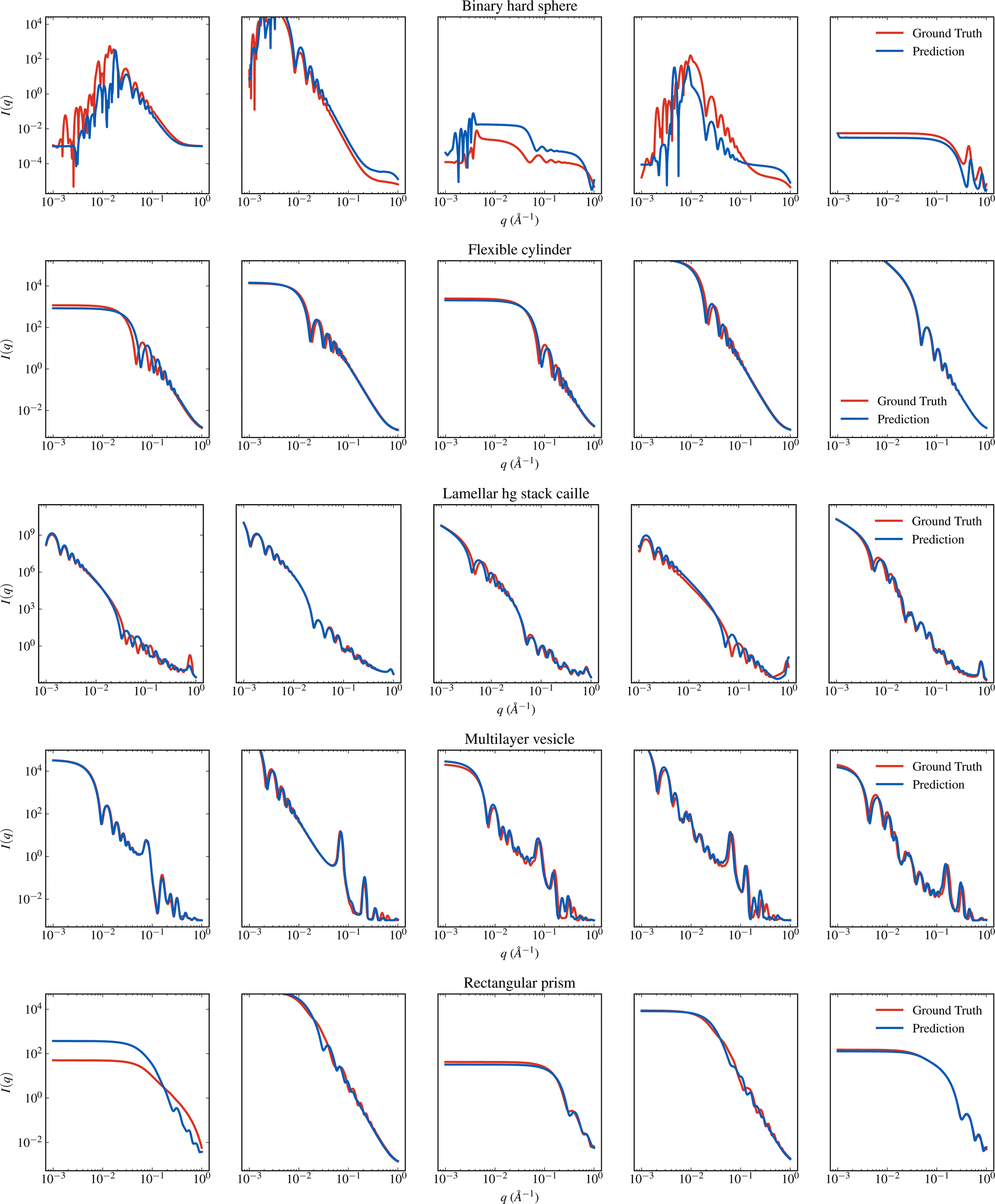 | ||
| Fig. 5 Visual comparison of I(q) generated from SASformer's parameter predictions to the true I(q) for several binary hard sphere, flexible cylinder, lamellar stack caille, multilayer vesicle and rectangular prism scattering models. See Fig. 4 for more details. | ||
Quantitatively, the performance of SASformer in predicting the scattering-model parameters was assessed using mean absolute error (MAE), mean absolute percentage error (MAPE) and the coefficient of determination (R2) calculated on samples in the test set. In each case, MAE is presented in the units of the parameter that is stated in the SasView Model Functions documentation. Given that the ranges of the parameters vary substantially, MAE can not be used to compare the performance of SASformer on different parameters. MAPE is a unitless quantity that enables this inter-parameter comparison. Full descriptions and definitions of these metrics are presented in the ESI.† The standard deviation and interquartile range (IQR) of the absolute errors are also reported to show the variability in the predictive distributions of each scattering-model parameter. Compared to the standard deviation, IQR provides a better description of the spread when data are not normally distributed.
Tables S5–S8 in the ESI† show the quantitative regression metrics, stratified by scattering-model class, for each parameter. To assess SASformer's ability to accurately predict each scattering-model parameter, we decide that parameters with a MAPE less than 0.25 (i.e., 25%) and R2 greater than 0.6 are those that SASformer predicts reasonably well. Of the 219 scattering-model parameters in the SAS-55M-20k dataset, SASformer achieves these desired results on 100 parameters. Using stricter cutoffs of less than 0.1 for MAPE and greater than 0.9 for R2, 59 scattering-model parameters meet these criteria. From these results, we can conclude that although SASformer performs well on a reasonably sized subset of parameters, there is room for improvement. Limited performance on the remaining parameters may be due to a variety of factors. For instance, the relatively lower performance observed in multi-shell models, such as core multi-shell or onion, can likely be attributed to their inherently increased complexity, which arises not only from the substantial number of parameters within these models but also from the intricate interdependencies among these parameters. While SASformer may encounter difficulty in predicting some of the available parameters, it is not designed as a substitute for the least-squares fitting method used to determine these parameters in practical applications. Instead, SASformer is intended to aid in this fitting process by proposing parameter ranges to test, potentially making it a valuable tool despite its limitations.
• Quotient transform, as described in the methods section of this work, where we take the log of the quotient transform of the square of I(q).
• Scalar neutralization, which is the cumulative product of the quotient transform of the square of I(q). A logarithm follows the cumulative product.
• Zero-index normalization, where we first square then take the logarithm of I(q) and divide the entire resulting sequence by its zeroth index value.
While the quotient transform changes the shape of the input scattering intensity, scalar neutralization restores its original shape by application of the cumulative product, removing any scale factors in the process. Zero-index normalization, which also preserves the original function's shape, is arguably the simplest transformation, and was used by Molodenskiy et al.8 and Archibald et al.7 in their work. We omit a comparison to dimensionally-reduced representations which do not make use of the full sequence, such as those used in works by Franke et al.,6 Lutz-Bueno et al.19 and others cited in 1.1. Our approach utilizes a transformer-based neural network, which capitalizes on the strengths of such models in processing and learning from features across the entire signal sequence.
For each model trained using the three scale-invariant representations and evaluated on the test dataset, Table 2 shows (a) the average of the accuracies of each scattering-model class; (b) the median of the MAPEs of scattering-model parameters (MdMAPE). The quotient transform results in the highest accuracy and lowest MdMAPE, while both the quotient transform and scalar neutralization methods significantly outperform zero-index normalization on accuracy. Zero-index normalization significantly outperforms scalar neutralization in terms of MdMAPE.
| Acc ↑ | MdMAPE ↓ | |
|---|---|---|
| Quotient transform | 0.957 | 0.297 |
| Scalar neutralization | 0.934 | 0.365 |
| Zero-index norm | 0.891 | 0.326 |
All three input transformations studied in this work are scale invariant, which provides a solution to the aforementioned problems of units and arbitrary scalars in real SAS intensities. However, it is worth highlighting that there may be cases where some quantities that we would like to predict depend on the scale of I(q). In these cases, scale invariant transformations like the quotient transform are insufficient since scale information is removed completely from the input. This suggests the possibility that a lack of scale in the input may be responsible for the inability of our model to predict some of the scattering-model parameters in Tables S5–S8† with any accuracy at all (as shown by the large MAPE and near-zero R2 values for some targets). This is plausible, but we leave the investigation of this for future work, as this requires the development of either an entirely new input representation or extending the model to additionally take scale information as input (alongside a scale-invariant representation of I(q)). Meanwhile, the results of this work are compelling as evidenced by the good fits observed on many of scattering-model classes.
3 Conclusions
The application of ML at the data-analysis stage of SAS experiments can assist researchers in the analysis of SAS data by suggesting scattering models that most probably represent their sample and predicting the parameters that best fit their experimental data. To this end, we have developed SASformer, a multi-task transformer-based neural network that jointly predicts scattering models classes and their parameters. This is in contrast to previous methods that only predicted the scattering model class. The use of a neural network allows the training and prediction of both classification and regression tasks efficiently in a single end-to-end model. The use of a transformer enables the masking of inputs, allowing experimental SAS intensities obtained at varying q-ranges to be seamlessly inputted into the model. Our method crucially employs a scale-invariant transformation of SAS intensities that is more accurate in scattering-model classification and results in smaller errors in scattering-model parameter estimation compared to other input representations that we tested. Our method was trained using a dataset, consisting of 1.1 million idealized and dilute SAS intensities with corresponding scattering-model classes and parameters, that we created specifically for this work. This has been made publicly available through this publication to ease and facilitate the development of ML methods on SAS data.As previously mentioned, a ML model such as ours could be integrated into SAS-data-analysis software. When experimental SAS data are loaded into the software, the data could be pre-processed and passed as input to the SASformer model, which provides a prediction of the top three scattering models that most probably represent the data and their parameters. Additionally, a software library with a simple application programming interface (API) that provides a pre-trained version of SASformer could allow users with large numbers of SAS-data files to obtain predictions of structural information in a high-throughput manner. This would be particularly useful for analyzing a huge amount of data that would otherwise be too arduous to analyze manually.
While our method stands to work well for SAXS data, performance on SANS data is likely to be slightly worse in comparison. This is due to q-resolution smearing, which occurs due to the unique geometries of SANS instruments. Consequently, data collected on a single unique sample using different SANS instruments would result in different scattering intensities where the sharpness of features would vary with peaks and fringes being broadened. During training of our model, batches of SAS intensities are sampled randomly in each training step. These could be smeared by convolving each I(q) with random instrument smearing parameters at each step. This would make the model robust to data from different SANS instruments and would avoid the need to create intractably large datasets that cover the configurations of all SANS instruments. Our method was trained on SAS data without noise, and it is likely that performance on noisy data would be slightly worse as a result. This could be solved in a similar manner to the aforementioned SANS data issue, by adding noise to each SAS intensity as batches are sampled during training. This would make the model resilient to noisy inputs. Additionally, since the data in the SAS-55M-20k dataset do not contain structure factors, it is unclear how the model would perform when faced with a SAS intensity function with a structure factor component. In the future, the scope of our method could be extended to enable the prediction of scattering intensities of multi-component systems, such as a system containing spherical scatterers with proportion p and cylindrical scatterers with proportion 1 − p, thus making it more general. This would additionally enable the prediction of structure-factor models and their parameters, and inter-particle distance-distribution information could be obtained as a result. Finally, uncertainty quantification could be enabled by defining the model as a Bayesian neural network31 which would allow a distribution of predictions to constructed from multiple stochastic outputs of the model. Conversely, conformal prediction methods,32,33 which can be applied to any underlying point predictor given the assumption of data exchangeability, could be employed to produce prediction regions or intervals and provide a more nuanced understanding of the uncertainties associated with the predictions.
Data availability
The code for SASformer and details on downloading the SAS-55M-20k dataset5 can be found at https://github.com/by256/sasformer.Author contributions
B. Y. conceived the project with guidance from J. M. C. and J. D. Under the supervision of J. M. C. and J. D., B. Y. wrote the code, designed the SASformer model architecture and input representation, created the SAS-55M-20k dataset and performed training and evaluation of the model. J. M. C. led the project in her role as PhD supervisor to B. Y., assisted by STFC advisor J. D. B. Y. drafted the paper with assistance from J. M. C. and J. D. All authors revised the manuscript and agreed upon its final version.Conflicts of interest
There are no conflicts to declare.Acknowledgements
J. M. C. is grateful for the BASF/Royal Academy of Engineering Research Chair in Data Driven Molecular Engineering of Functional Materials. J. M. C. is also indebted to the Science and Technology Facilities Council (STFC) via the ISIS Neutron and Muon Source who partly support this Research Chair and provide PhD studentship support (for B. Y.). The authors thank the Argonne Leadership Computing Facility, which is a DOE Office of Science Facility, for use of its research resources, under contract no. DE-AC02-06CH11357. This work benefited from the use of the SasView application, originally developed under NSF award DMR-0520547. SasView contains code developed with funding from the European Union's Horizon 2020 research and innovation programme under the SINE2020 project, grant agreement no. 654000.Notes and references
- A. Guinier, G. Fournet and K. L. Yudowitch, Small-Angle Scattering of X-Rays, Wiley, New York, 1955 Search PubMed.
- C. M. Jeffries, J. Ilavsky, A. Martel, S. Hinrichs, A. Meyer, J. S. Pedersen, A. V. Sokolova and D. I. Svergun, Nat. Rev. Methods Primers, 2021, 1, 70 CrossRef CAS.
- L. A. Feigin and D. I. Svergun, Structure Analysis by Small-Angle X-Ray and Neutron Scattering, Springer, New York, 1987 Search PubMed.
- R. Pecora, Dynamic Light Scattering: Applications of Photon Correlation Spectroscopy, Springer, New York, 1985 Search PubMed.
- B. Yildirim, J. Doutch and J. M. Cole, SAS-55M-20k: 1.1 Million Theoretical Small-Angle Scattering Intensities, 2024 DOI:10.6084/m9.figshare.21716618.
- D. Franke, C. M. Jeffries and D. I. Svergun, Biophys. J., 2018, 114, 2485–2492 CrossRef CAS PubMed.
- R. K. Archibald, M. Doucet, T. Johnston, S. R. Young, E. Yang and W. T. Heller, J. Appl. Crystallogr., 2020, 53, 326–334 CrossRef CAS.
- D. S. Molodenskiy, D. I. Svergun and A. G. Kikhney, Structure, 2022, 30, 900–908 CrossRef CAS PubMed.
- P. Tomaszewski, S. Yu, M. Borg and J. Rönnols, Computing Research Repository (CoRR), 2021, abs/2111.08645 Search PubMed.
- Z. Chen, N. Andrejevic, N. C. Drucker, T. Nguyen, R. P. Xian, T. Smidt, Y. Wang, R. Ernstorfer, D. A. Tennant, M. Chan and M. Li, Chem. Phys. Rev., 2021, 2, 031301 CrossRef.
- M. Doucet, A. M. Samarakoon, C. Do, W. T. Heller, R. Archibald, D. A. Tennant, T. Proffen and G. E. Granroth, Machine Learning: Science and Technology, 2020, 2, 023001 Search PubMed.
- M. Doucet, R. K. Archibald and W. T. Heller, Machine Learning: Science and Technology, 2021, 2, 035001 Search PubMed.
- C.-H. Tung, S.-Y. Chang, H.-L. Chen, Y. Wang, K. Hong, J. M. Carrillo, B. G. Sumpter, Y. Shinohara, C. Do and W.-R. Chen, J. Chem. Phys., 2022, 156, 131101 CrossRef CAS PubMed.
- N. C. Drucker, T. Liu, Z. Chen, R. Okabe, A. Chotrattanapituk, T. Nguyen, Y. Wang and M. Li, Synchrotron Radiation News, 2022, 1–5 Search PubMed.
- H. Abdel Aty, R. Strutt, N. Mcintyre, M. Allen, N. E. Barlow, M. Páez-Pérez, J. M. Seddon, N. Brooks, O. Ces and I. R. Gould, Digital Discovery, 2022, 1, 98–107 RSC.
- C. Do, W.-R. Chen and S. Lee, MRS Adv., 2020, 5, 1577–1584 CrossRef CAS.
- A. Hinderhofer, A. Greco, V. Starostin, V. Munteanu, L. Pithan, A. Gerlach and F. Schreiber, J. Appl. Crystallogr., 2023, 56, 3–11 CrossRef CAS.
- M. Röding, P. Tomaszewski, S. Yu, M. Borg and J. Rönnols, Front. Mater., 2022, 9 DOI:10.3389/fmats.2022.956839/full.
- V. Lutz-Bueno, C. Arboleda, L. Leu, M. J. Blunt, A. Busch, A. Georgiadis, P. Bertier, J. Schmatz, Z. Varga, P. Villanueva-Perez, Z. Wang, M. Lebugle, C. David, M. Stampanoni, A. Diaz, M. Guizar-Sicairos and A. Menzel, J. Appl. Crystallogr., 2018, 51, 1378–1386 CrossRef CAS.
- K. Vaddi, K. Li and L. D. Pozzo, Digital Discovery, 2023, 2, 1471–1483 RSC.
- D. Svergun, C. Barberato and M. H. J. Koch, J. Appl. Crystallogr., 1995, 28, 768–773 CrossRef CAS.
- K. T. Butler, M. D. Le, J. Thiyagalingam and T. G. Perring, J. Phys.: Condens. Matter, 2021, 33, 194006 CrossRef CAS PubMed.
- C. M. Heil, Y. Ma, B. Bharti and A. Jayaraman, JACS Au, 2023, 3, 889–904 CrossRef CAS PubMed.
- A. Vaswani, N. Shazeer, N. Parmar, J. Uszkoreit, L. Jones, A. N. Gomez, L. Kaiser and I. Polosukhin, Computing Research Repository (CoRR), 2017, abs/1706.03762 Search PubMed.
- A. Jaegle, F. Gimeno, A. Brock, A. Zisserman, O. Vinyals and J. Carreira, Computing Research Repository (CoRR), 2021, abs/2103.03206 Search PubMed.
- A. Jaegle, S. Borgeaud, J. Alayrac, C. Doersch, C. Ionescu, D. Ding, S. Koppula, D. Zoran, A. Brock, E. Shelhamer, O. J. Hénaff, M. M. Botvinick, A. Zisserman, O. Vinyals and J. Carreira, Computing Research Repository (CoRR), 2021, abs/2107.14795 Search PubMed.
- T. B. Brown, B. Mann, N. Ryder, M. Subbiah, J. Kaplan, P. Dhariwal, A. Neelakantan, P. Shyam, G. Sastry, A. Askell, S. Agarwal, A. Herbert-Voss, G. Krueger, T. Henighan, R. Child, A. Ramesh, D. M. Ziegler, J. Wu, C. Winter, C. Hesse, M. Chen, E. Sigler, M. Litwin, S. Gray, B. Chess, J. Clark, C. Berner, S. McCandlish, A. Radford, I. Sutskever and D. Amodei, Computing Research Repository (CoRR), 2020, abs/2005.14165 Search PubMed.
- M. Shoeybi, M. Patwary, R. Puri, P. LeGresley, J. Casper and B. Catanzaro, Computing Research Repository (CoRR), 2019, abs/1909.08053 Search PubMed.
- L. Chen, K. Lu, A. Rajeswaran, K. Lee, A. Grover, M. Laskin, P. Abbeel, A. Srinivas and I. Mordatch, Computing Research Repository (CoRR), 2021, abs/2106.01345 Search PubMed.
- M. Janner, Q. Li and S. Levine, Computing Research Repository (CoRR), 2021, abs/2106.02039 Search PubMed.
- Y. Gal and Z. Ghahramani, Proceedings of the 33rd International Conference on Machine Learning, New York, USA, 2016, pp. 1050–1059 Search PubMed.
- H. Papadopoulos, K. Proedrou, V. Vovk and A. Gammerman, Machine Learning: ECML 2002, 2002, pp. 345–356 Search PubMed.
- J. Lei and L. Wasserman, Journal of the Royal Statistical Society Series B: Statistical Methodology, 2013, 76, 71–96 CrossRef.
Footnote |
| † Electronic supplementary information (ESI) available. See DOI: https://doi.org/10.1039/d3dd00225j |
| This journal is © The Royal Society of Chemistry 2024 |