
 Open Access Article
 This Open Access Article is licensed under a Creative Commons Attribution-Non Commercial 3.0 Unported Licence
Derivative-based pre-training of graph neural networks for materials property predictions†
Shuyi
Jia
 a,
Akaash R.
Parthasarathy
a,
Rui
Feng
a,
Guojing
Cong
b,
Chao
Zhang
a and
Victor
Fung
*a
a,
Akaash R.
Parthasarathy
a,
Rui
Feng
a,
Guojing
Cong
b,
Chao
Zhang
a and
Victor
Fung
*a
aComputational Science and Engineering, Georgia Institute of Technology, Atlanta, GA, USA. E-mail: victorfung@gatech.edu
bOak Ridge National Laboratory, Oak Ridge, TN, USA
First published on 21st February 2024
Abstract
While pre-training has transformed many fields in deep learning tremendously, its application to three-dimensional crystal structures and materials science remains limited and under-explored. In particular, devising a general pre-training objective which is transferable to many potential downstream tasks remains challenging. In this paper, we demonstrate the benefits of pre-training graph neural networks (GNNs) with the objective of implicitly learning an approximate force field via denoising, or explicitly via supervised learning on energy, force, or stress labels. For implicit learning of the force field, we find there are significant benefits to training the model on the derivatives of the output, rather than on the output itself. We further show an explicit training of the force field using labelled data yields an even greater benefit than implicit training, and similarly benefits from a derivative-based training objective. We find that overall, the best pre-training performance can be achieved by explicitly learning the full combination of energy, force, and stress labels using output derivatives. This pre-training approach is advantageous as it leverages readily available forces from non-equilibrium structures produced during ab initio calculations, enabling the usage of significantly larger datasets for pre-training than using only equilibrium structures in denoising. We demonstrate the effectiveness of this approach on a wide range of materials property benchmarks across many materials systems and properties. These results suggest exciting future opportunities for scaling up pre-training on GNNs to build foundational models in materials science.
1. Introduction
In the realm of artificial intelligence (AI), pre-training1,2 stands as a pivotal technique that has revolutionized the landscape of an array of different deep learning tasks, most prominently in the fields of natural language processing (NLP)3–5 and computer vision (CV).6–8 At its core, pre-training involves training neural network models on large datasets to learn meaningful underlying features and structures. Subsequently, the pre-trained models can be finetuned for specific downstream tasks that usually involve datasets at a much smaller scale. While large-scale pre-trained models have underpinned the remarkable success we see today in natural language and vision, its application in materials science remains limited and largely unexplored despite considerable efforts being directed toward the design and invention of novel graph neural network (GNN) architectures to better represent the intricate 3D geometries and atomic interactions present in materials.9–13Recent advancements in pre-training in molecular and materials science can be primarily categorized into two learning paradigms: transfer learning and self-supervised learning. In the case of transfer learning, neural network models are first trained on large datasets with specific target properties before being finetuned on downstream tasks.14,15 In comparison, pre-training via self-supervised learning does not rely on explicit labels, but uses surrogate tasks to generate its own training data. Such pre-training tasks include context prediction and attribute masking.16,17 Additionally, a subset of self-supervised learning known as contrastive learning has emerged recently as a popular framework for pre-training. Specifically, contrastive learning relies on learning representations by contrasting self-generated positive and negative samples given an input graph. By doing so, the model can acquire a more discriminative and generalizable representation, thereby yielding remarkable performance in molecular and materials property prediction.18–21
Recently, a novel pre-training technique for 3D structures based on denoising achieved state-of-the-art (SOTA) performance on multiple molecular benchmarks.22 Specifically, the goal of pre-training, referred to as the denoising objective, is to predict the amount of i.i.d. noise added to the spatial coordinates of 3D molecular structures at equilibrium. Relying on the connection between denoising autoencoders and score-matching,23–25 it can also be shown that such a denoising objective is equivalent to implicitly learning an approximate force field. The empirical success of pre-training via denoising indicates that implicitly learning a force field does translate to learning better and meaningful representations for downstream tasks. However, the question persists as to whether explicitly learning the force field would lead to comparable, if not superior, performance. Additionally, a drawback of pre-training via denoising is the requirement of the upstream dataset to consist solely of equilibrium structures, e.g. structures at energy minima.
Inspired by the denoising approach,22 in this work, we focus on the problem of pre-training GNNs with the objective of learning an approximate force field, which can be learnt in two ways, implicitly and explicitly. Pre-training via denoising is an example of the former, and our approach—derivative-based pre-training with forces—illustrates the explicit method. In the context of our work, derivative-based specifically denotes the process of obtaining model predictions by differentiating model outputs with respect to atomic positions. Concretely, in our approach, we optimize a GNN to directly minimize the loss between model derivatives and forces on 3D structures. In practice, additional graph-level objectives such as energies and stress are also incorporated to learn more meaningful representations during pre-training. It is also worth noting that while the original pre-training via denoising adopts a node-level noise prediction head, it can be made into a derivative-based form by equating noise to model derivatives with respect to atomic positions.26
The motivation behind our work is as follows. First, in materials chemistry, the majority of computational datasets available are acquired through ab initio calculations like density functional theory (DFT). A noteworthy aspect is that during the generation of equilibrium structures via DFT, numerous non-equilibrium structures with forces are also produced. This means that forces can be regarded as readily available labels, eliminating the strict requirement of equilibrium structures for pre-training through denoising. Second, the absence of constraints posed by pre-training methods which use only equilibrium structures allows us to capitalize on significantly larger datasets that include forces, presenting a valuable and exciting opportunity for scaling up pre-training to build foundational models in materials science. Additionally, while the learning of a force field with interatomic forces and additional attributes such as energies and stress is an established approach,13,27 its application as a pre-training strategy remains largely under-explored. Importantly, prior research on interatomic potentials predominantly focuses on tasks such as structure relaxation and dynamics simulations. In contrast, our approach distinctly investigates the advantages of pre-training with forces for downstream target property prediction.
Our contributions can be summarized as follows. Firstly, we establish that derivative-based pre-training via denoising outperforms its non-derivative-based counterpart, which relies on a prediction head, in downstream property prediction tasks. Secondly, we demonstrate the consistently better performance of our pre-training approach-derivative-based pre-training with forces and additional objectives-across an extensive array of materials property benchmarks when compared to both denoising variants. These findings underscore the advantages of explicit learning over implicit learning of the underlying approximate force field.
2. Methodology
2.1 Background
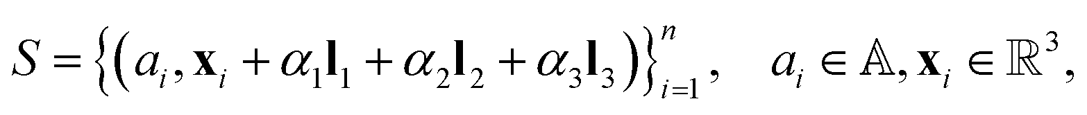
The representation of an arbitrary material structure or crystal can be condensed into a minimum image of atoms positioned in 3D space. This minimum image, also known as the unit cell, can be repeated infinitely in the x, y, and z directions to reveal the periodic nature of the structure. Given a structure S with n atoms in its unit cell, the system can be fully described by: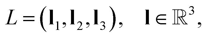 | (1) |
 | (2) |
 is the set of all chemical elements and x is the 3D coordinates. Note that α1, α2, and α3 are integers that translate the unit cell using L in all directions. If α1 = α2 = α3 = 0, we have the unit cell at an arbitrary center in space.
2.2 Pre-training via denoising
Given a dataset of M material structures, we pre-train a graph neural network gθ with parameters θ via the denoising objective which, at its core, entails predicting the amount of noise added to the 3D coordinates of structures. Note that the subscript eq on the dataset
  is used to indicate that this dataset contains structures at equilibrium only. Such a distinction is needed since, as mentioned earlier, pre-training via denoising requires structures at equilibrium per the original formulation.22 Specifically, we have
 | (3) |
 are the forces on each atom in a given S.
Concretely, the denoising objective requires us to first perturb each structure  by adding i.i.d. Gaussian noise to each atom's coordinates. In other words, we generate a noisy copy of S, denoted
  by:
by:
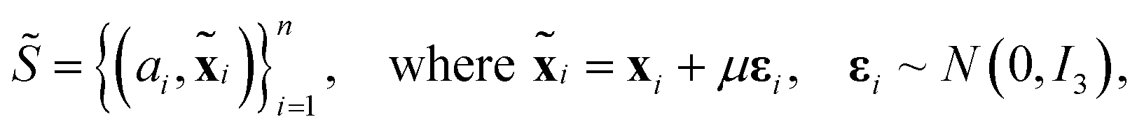 | (4) |
 | (5) |
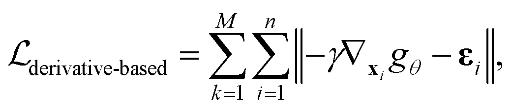
2.3 Derivative-based pre-training with forces
To explicitly learn a force field given a dataset containing N crystal structures at both equilibrium and non-equilibrium, we note that the force on any atom can be obtained by taking the derivative of the potential energy with respect to the atomic position: f = −∇xU. Thus, given the model
  that maps from the input space
  to the energy space
  the pre-training with forces loss can be expressed as:
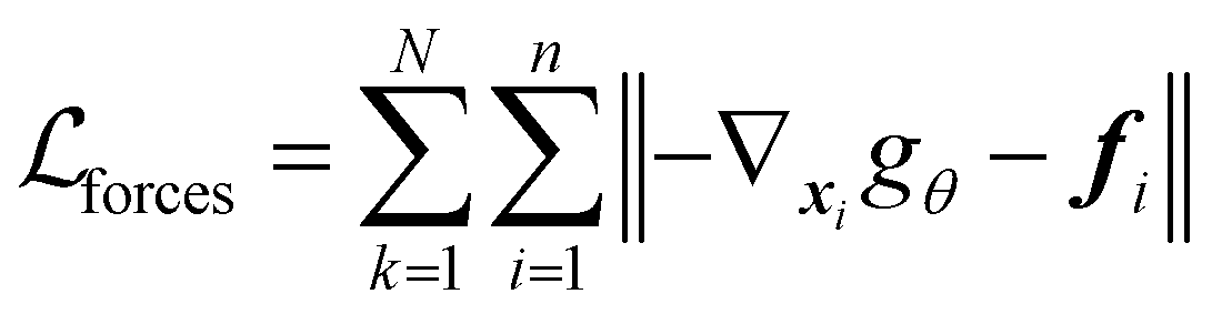 | (6) |
 | (7) |
Fig. 1 provides an overview of our pre-training strategy.
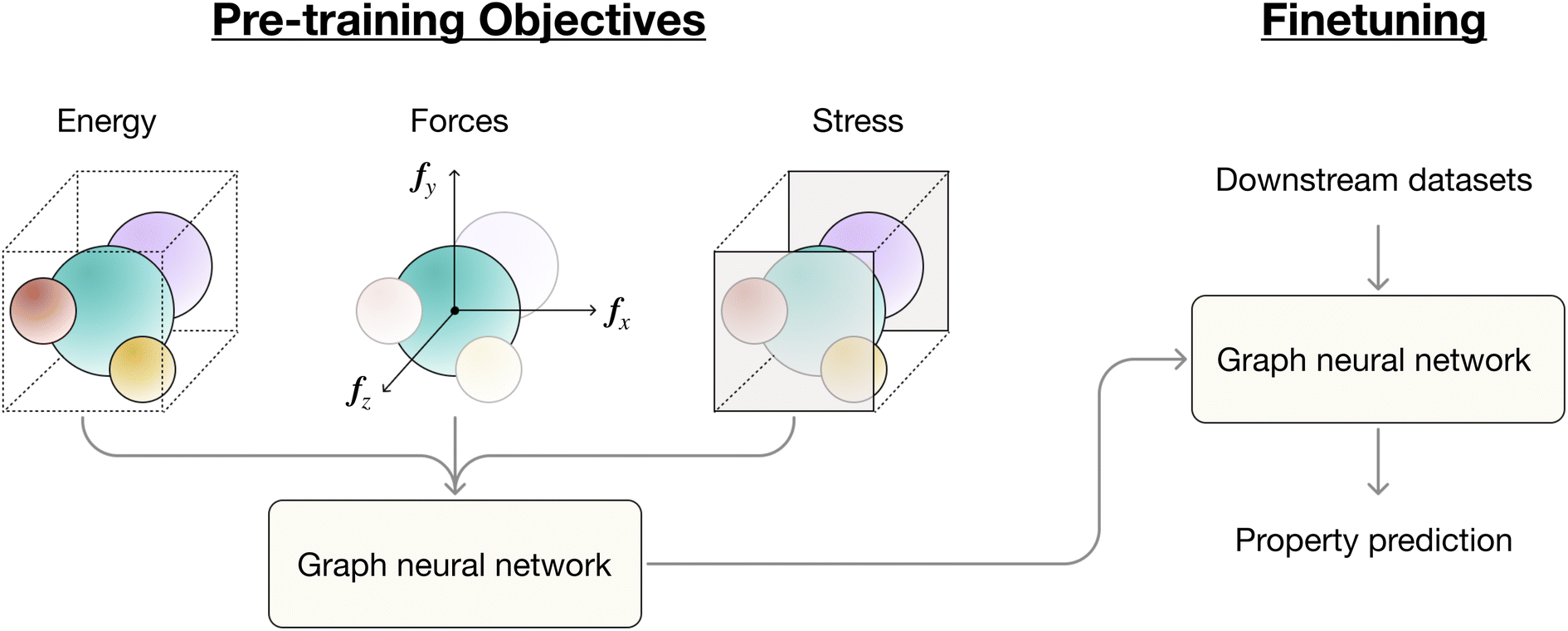 | ||
| Fig. 1 An overview of derivative-based pre-training of graph neural networks (GNNs) with forces and additional graph-level labels including energy and stress. During the pre-training phase, the model generates scalar energy values. Predictions for forces and stress are obtained by differentiating the energy with respect to atomic positions and cell vectors respectively. In practice, our pre-training objectives can be a combination of any of the three: forces, energy and stress. In the fine-tuning phase, we train a GNN model loaded with the pre-trained weights to predict a given target property. | ||
2.4 Graph neural networks
Given that our pre-training strategy is model-agnostic and can, in theory, be applied to any neural network model for graphs, we have chosen two representative models, CGCNN28 and TorchMD-Net29 for illustrative purposes. The former is a classic message-passing GNN model which has been successfully applied to molecules and materials on many property prediction tasks. The latter is a more recently developed model based on the equivariant transformer architecture that has achieved SOTA results on datasets such as QM9.303. Results and discussion
3.1 Datasets
Our upstream dataset for derivative-based pre-training with forces, which we shall henceforth refer to as “MP forces,” consists of 187![[thin space (1/6-em)]](https://www.rsc.org/images/entities/char_2009.gif) 687 structures with energies, forces, and stress properties obtained from structural relaxations performed by the materials project.27 A subset of this dataset encompassing a collection of 62783 structures at equilibrium is further curated for pre-training via denoising. We label this subset as “MP forces relaxed”. It is worth noting that while the computational cost of generating MP forces and MP forces relaxed is the same, we have about 200% more structures in the former. The availability of this immense reservoir of additional training samples serves as the pivotal driving force behind our work.
687 structures with energies, forces, and stress properties obtained from structural relaxations performed by the materials project.27 A subset of this dataset encompassing a collection of 62783 structures at equilibrium is further curated for pre-training via denoising. We label this subset as “MP forces relaxed”. It is worth noting that while the computational cost of generating MP forces and MP forces relaxed is the same, we have about 200% more structures in the former. The availability of this immense reservoir of additional training samples serves as the pivotal driving force behind our work.
The finetuning performance of the pre-training strategies is tested on a wide variety of properties including those in the MatBench suite.31 Specifically, we have chosen 8 properties, namely exfoliation energy, frequency at last phonon PhDOS peak, refractive index, shear and bulk modulus, formation energy, and band gap. We have also included a dataset containing two-dimensional materials (2D materials) with work function as the target property,32 a dataset containing crystal structures of metal–organic frameworks (MOFs) with band gap as the target property,33 and a dataset containing metal alloy surfaces (surface) with adsorption energy as the target property.34
An overview of the finetuning datasets used is provided in Table 1.
| Dataset | # Structures | Property | Unit |
|---|---|---|---|
| JDFT | 636 | Exfoliation energy | meV per atom |
| Phonons | 1265 | Freq. at last phonon PhDOS peak | 1 cm |
| Dielectric | 4764 | Refractive index | — |
| (log) GVRH | 10987 |
Shear modulus | GPa |
| (log) KVRH | 10987 |
Bulk modulus | GPa |
| Perovskite | 18928 |
Formation energy | eV per atom |
| MP form | 132752 |
Formation energy | eV per atom |
| MP gap | 106113 |
Band gap | eV |
| 2D | 3814 | Work function | eV |
| MOF | 13058 |
Band gap | eV |
| Surface | 37334 |
Adsorption energy | eV |
3.2 Training setup
CGCNN and TorchMD-Net are both implemented in PyTorch35 as part of the MatDeepLearn package.36 All finetuning experiments are averaged over 5 runs. A train:validation:test split ratio of 0.6:0.2:0.2 is applied to every downstream dataset. Detailed hyperparameter and hardware settings can be found in ESI Appendix A.†
3.3 Results
We first evaluate our pre-training strategy—derivative-based pre-training with forces—and the two different variants of pre-training via denoising,22 prediction head denoising and derivative-based denoising, on the eleven datasets shown in Table 1. Furthermore, pre-training with forces is evaluated on a set of different weights λ, as defined in eqn (7). Without much ambiguity, it should be understood that the ratio λenergy:λforces:λstress refers to the respective weights on the losses of energy, forces, and stress for models pre-trained with our strategy. In total, 5 different ratios of λenergy:λforces:λstress are used for pre-training with forces: 1:0:0, 0:1:0, 0:1:1, 1:1:1, and 1:500:500.
The finetuning results of both pre-training strategies on CGCNN28 are shown in Table 2. We first observe that both derivative-based denoising and prediction head denoising fail to beat the baseline with negative average percentage improvements of −6.98% and −7.71% respectively. However, if we exclude the anomalously high MAE on the phonons dataset, the average percentage improvements in MAE for the two variants of denoising become 3.13% and −6.84% respectively. This suggests that derivative-based denoising outperforms its non-derivative-based counterpart in terms of fine-tuning performance. A similar trend is evident in the results obtained using the TorchMD-Net model, as detailed in the subsequent paragraphs. It should be highlighted that prediction head denoising experiences a significant loss plateau early in the pre-training phase, which might have led to dissimilar atomic representations under principal component analysis compared to other pre-training strategies and variants (see ESI Appendix D†).
| JDFT | Phonons | Dielectric | GVRH | KVRH | Perovskites | 2D | MOF | Surface | MP gap | MP form | Avg. % impr. | ||
|---|---|---|---|---|---|---|---|---|---|---|---|---|---|
| Baseline | 62.6 | 59.1 | 0.406 | 0.105 | 0.0736 | 0.0437 | 0.263 | 0.343 | 0.0852 | 0.230 | 0.0417 | — | |
| Forces | 1:0:0 |
46.5 | 57.6 | 0.380 | 0.098 | 0.0728 | 0.0365 | 0.212 | 0.297 | 0.0743 | 0.218 | 0.0380 | 10.8% |
| 0:1:0 |
50.5 | 63.7 | 0.338 | 0.111 | 0.0942 | 0.0401 | 0.240 | 0.319 | 0.0809 | 0.230 | 0.0443 | 1.58% | |
| 0:1:1 |
56.4 | 67.9 | 0.377 | 0.103 | 0.0777 | 0.0411 | 0.232 | 0.311 | 0.0800 | 0.226 | 0.0406 | 3.28% | |
| 1:1:1 |
48.9 | 56.4 | 0.248 | 0.0945 | 0.0709 | 0.0370 | 0.213 | 0.296 | 0.0741 | 0.210 | 0.0383 | 14.3% | |
| 1:500:500 |
45.5 | 60.7 | 0.324 | 0.0962 | 0.0720 | 0.0366 | 0.209 | 0.291 | 0.0747 | 0.212 | 0.0392 | 12.1% | |
| Derivative-based denoising | 46.5 | 123.0 | 0.386 | 0.0947 | 0.0743 | 0.0389 | 0.212 | 0.473 | 0.0883 | 0.227 | 0.0410 | −6.98% (3.13%) | |
| Prediction head denoising | 59.0 | 68.8 | 0.376 | 0.109 | 0.0933 | 0.0437 | 0.278 | 0.417 | 0.0965 | 0.228 | 0.0464 | −7.71% (−6.84%) | |
| Best % impr. | 27.3% | 4.57% | 38.9% | 10.0% | 3.67% | 16.5% | 20.5% | 15.2% | 13.0% | 8.70% | 8.87% | — | |
Next, we observe that derivative-based pre-training with forces and additional objectives yields superior performance across all downstream datasets. Specifically, the average percentage improvement in MAE in comparison to the baseline ranges from 1.58% (ratio 0:1:0) to as high as 14.3% (ratio 1:1:1). In addition, we note that our pre-training strategy not only consistently outperforms the baseline but also surpasses both variants of pre-training via denoising. Interestingly, the ratios 1:1:1 and 1:500:500 almost always yield the best results, doing so for 9 of the 11 datasets tested. In comparison, pre-training with forces alone, e.g. 0:1:0, struggles to outperform the baseline on datasets like JDFT, GVRH, and KVRH.
To show that derivative-based pre-training with forces is model-agnostic and can be beneficial beyond CGCNN, we applied the same pre-training strategies to the TorchMD-Net architecture.29 TorchMD-Net is an equivaraint transformer whose layers maintain per-atom scalar features and vector features that are updated by a self-attention mechanism. Similar to CGCNN, we first obtain a scalar output from the model before auto-differentiating with respect to positions to obtain forces or noise predictions for derivative-based approaches.
In Table 3, we evaluate the finetuning performance of derivative-based pre-training with forces and pre-training via denoising on the TorchMD-Net architecture. First, we observe that both variants of denoising beat the baseline, with derivative-based denoising emerging as the better option, achieving an average percentage improvement in MAE of 23.5%. Similar to what we have observed in the case of CGCNN, derivative-based pre-training with forces significantly improves over the baseline for an average percentage improvement in MAE ranging from 15.1% (ratio 1:0:0) to 25.1% (ratio 1:500:500). We also observe that our pre-training strategy performs better than or equal to pre-training via denoising for 10 out of 11 datasets. The only exception is the JDFT dataset, where the MAE for derivative-based denoising is lower than the best performing ratio of pre-training with forces by 0.4.
| JDFT | Phonons | Dielectric | GVRH | KVRH | Perovskites | 2D | MOF | Surface | MP gap | MP form | Avg. % impr. | ||
|---|---|---|---|---|---|---|---|---|---|---|---|---|---|
| Baseline | 55.7 | 117 | 0.415 | 0.107 | 0.0840 | 0.0440 | 0.287 | 0.265 | 0.0774 | 0.231 | 0.0351 | — | |
| Forces | 1:0:0 |
57.6 | 108 | 0.364 | 0.0830 | 0.0616 | 0.0416 | 0.190 | 0.260 | 0.0579 | 0.195 | 0.0287 | 15.1% |
| 0:1:0 |
51.0 | 111 | 0.320 | 0.0805 | 0.0596 | 0.0338 | 0.186 | 0.239 | 0.0528 | 0.164 | 0.0240 | 22.8% | |
| 0:1:1 |
47.4 | 111 | 0.317 | 0.0800 | 0.0597 | 0.0355 | 0.180 | 0.238 | 0.0518 | 0.168 | 0.0250 | 23.1% | |
| 1:1:1 |
50.9 | 105 | 0.306 | 0.0798 | 0.0608 | 0.0395 | 0.189 | 0.245 | 0.0531 | 0.194 | 0.0261 | 20.3% | |
| 1:500:500 |
39.0 | 109 | 0.272 | 0.0759 | 0.0569 | 0.0356 | 0.185 | 0.246 | 0.0540 | 0.179 | 0.0250 | 25.1% | |
| Derivative-based denoising | 38.6 | 111 | 0.331 | 0.0770 | 0.0572 | 0.0371 | 0.180 | 0.241 | 0.0534 | 0.177 | 0.0259 | 23.5% | |
| Prediction head denoising | 46.0 | 128 | 0.353 | 0.0829 | 0.0592 | 0.0368 | 0.194 | 0.242 | 0.0536 | 0.179 | 0.0272 | 18.9% | |
| Best % impr. | 30.7% | 10.3% | 34.5% | 29.1% | 32.3% | 19.3% | 37.3% | 10.2% | 33.1% | 29.0% | 31.6% | — | |
Furthermore, it is worth noting that when the TorchMD-Net model is pre-trained with forces alone (ratio 0:1:0), we observe a substantial average percentage improvement of 22.8% on the fine-tuning datasets. This improvement is significantly higher compared to the previously achieved 1.58% with CGCNN. Considering results from both CGCNN and TorchMD-Net, it becomes evident that the most effective pre-training strategy involves a combination of node-level and graph-level objectives. This is substantiated by the consistently strong performance observed with ratios such as 1:1:1 and 1:500:500.
| JDFT | Phonons | Dielectric | GVRH | KVRH | Perovskites | 2D | MOF | Surface | MP gap | MP form | Avg. % impr. | ||
|---|---|---|---|---|---|---|---|---|---|---|---|---|---|
| Baseline | 62.3 | 59.5 | 0.355 | 0.0947 | 0.0681 | 0.0437 | 0.254 | 0.315 | 0.0821 | 0.223 | 0.0402 | — | |
| Forces | 1:0:0 |
42.2 | 54.6 | 0.313 | 0.0921 | 0.0677 | 0.0364 | 0.208 | 0.299 | 0.0752 | 0.215 | 0.0395 | 9.94% |
| 0:1:0 |
42.3 | 51.0 | 0.332 | 0.102 | 0.0746 | 0.0403 | 0.249 | 0.302 | 0.0758 | 0.225 | 0.0363 | 6.00% | |
| 0:1:1 |
49.5 | 49.5 | 0.360 | 0.0993 | 0.0738 | 0.0400 | 0.267 | 0.301 | 0.0753 | 0.217 | 0.0345 | 5.06% | |
| 1:1:1 |
46.9 | 41.7 | 0.255 | 0.0887 | 0.0659 | 0.0360 | 0.204 | 0.295 | 0.0730 | 0.212 | 0.0353 | 14.9% | |
| 1:500:500 |
39.6 | 44.4 | 0.309 | 0.0932 | 0.0715 | 0.0357 | 0.205 | 0.289 | 0.0694 | 0.210 | 0.0322 | 14.4% | |
| Derivative-based denoising | 41.2 | 55.1 | 0.287 | 0.0873 | 0.0661 | 0.0370 | 0.185 | 0.291 | 0.0739 | 0.212 | 0.0326 | 14.1% | |
| Best % impr. | 36.4% | 29.9% | 28.2% | 7.81% | 3.23% | 18.3% | 27.2% | 8.25% | 15.5% | 5.83% | 19.9% | — | |
We observe that there is a general increase in performance over the baseline when global mean pooling is used. Derivative-based pre-training with forces performs the best for 9 of 11 datasets with an average percentage improvement in MAE ranging from 5.06% (ratio 0:1:1) to 14.9% (ratio 1:1:1). Compared to the range of 1.58% to 14.3% when add pooling is applied to our pre-training strategy, we note that there is an improvement in both the lower and upper bounds. Further, derivative-based denoising with mean pooling beats the baseline by as high as 14.1% on average, which is significantly better considering the fact that it fails to beat the baseline with add pooling. Such a huge improvement stems from the significant decrease in MAE for phonons and MP formation energy. More importantly, this shows that derivative-based pre-training with forces and derivative-based denoising can be beneficial regardless of the type of pooling used in downstream tasks.
:1:0 and 1:500:500 variants of the derivative-based pre-training with forces strategy for demonstration purposes. 0:1:0 was chosen to ascertain whether the finetuning performance of pre-training with solely force labels aligns with how well the pre-trained model has converged while 1:500:500 was chosen due to its consistent and superior overall performance.
In Table 5, we evaluate the 0:1:0 and 1:500:500 variants with 5 different number of epochs: 12, 25, 50, 100, and 200. In general, we observe that as the number of pre-training epochs increases, the greater the decrease is in MAE during finetuning. This trend is most evident in the case of ratio 1:500:500—finetuning results obtained from the model pre-trained for 200 epochs are the best for 9 of 11 datasets. The same decrease of MAE with an increase in the number of epochs for pre-training is observed in the case of ratio 0:1:0, albeit less consistent. This observation underscores the direct relationship between the level of convergence achieved by the pre-trained model and the subsequent improvement in downstream finetuning performance.
| Ratio | # Epochs | JDFT | Phonons | Dielectric | GVRH | KVRH | Perovskites | 2D | MOF | Surface | MP gap | MP form |
|---|---|---|---|---|---|---|---|---|---|---|---|---|
| 0:1:0 |
12 | 46.6 | 77.3 | 0.345 | 0.106 | 0.0759 | 0.0426 | 0.255 | 0.327 | 0.0823 | 0.229 | 0.0408 |
| 25 | 54.3 | 70.3 | 0.319 | 0.103 | 0.0749 | 0.0417 | 0.249 | 0.328 | 0.0816 | 0.227 | 0.0417 | |
| 50 | 48.7 | 72.9 | 0.365 | 0.106 | 0.0749 | 0.0406 | 0.245 | 0.357 | 0.0801 | 0.230 | 0.0414 | |
| 100 | 50.5 | 63.7 | 0.338 | 0.111 | 0.0942 | 0.0401 | 0.240 | 0.319 | 0.0809 | 0.230 | 0.0443 | |
| 200 | 52.3 | 66.7 | 0.368 | 0.107 | 0.0778 | 0.0399 | 0.233 | 0.320 | 0.0776 | 0.227 | 0.0394 | |
| 1:500:500 |
12 | 46.7 | 59.8 | 0.343 | 0.116 | 0.0761 | 0.0392 | 0.241 | 0.311 | 0.0799 | 0.229 | 0.0411 |
| 25 | 49.0 | 65.8 | 0.324 | 0.102 | 0.0790 | 0.0383 | 0.220 | 0.305 | 0.0802 | 0.228 | 0.0407 | |
| 50 | 46.4 | 78.0 | 0.346 | 0.102 | 0.0727 | 0.0369 | 0.213 | 0.299 | 0.0762 | 0.220 | 0.0387 | |
| 100 | 45.5 | 85.8 | 0.324 | 0.0962 | 0.0720 | 0.0366 | 0.208 | 0.291 | 0.0747 | 0.212 | 0.0392 | |
| 200 | 38.1 | 59.9 | 0.320 | 0.0949 | 0.0708 | 0.0351 | 0.200 | 0.287 | 0.0730 | 0.215 | 0.0343 |
Overall, we observe that derivative-based pre-training with forces consistently outperforms both variants of the denoising approach, highlighting the effectiveness of explicitly learning a force field for downstream property prediction tasks. Beyond its superior finetuning performance, another advantage of pre-training with forces is its compatibility with non-equilibrium structures during training, thereby allowing the use of diverse datasets. However, a limitation of this approach is its dependency on datasets with forces as labels, which could pose challenges in obtaining such labeled data for specific domains or applications. On the other hand, pre-training via denoising, being self-supervised, is in theory applicable to a broader range of datasets. However, in reality, a significant drawback of the denoising approach is its need of training structures to be at equilibrium, a requirement that might be prohibitively expensive to satisfy and limit the approach's generalizability to non-equilibrium structures.
In a concurrent study similar to this work, Shoghi et al.37 explore the effectiveness of pre-training with forces for atomic property prediction. Notably, their methodology involves supervised pre-training with forces and energies, utilizing an expansive pre-training dataset comprising 120 million samples. The models used by Shoghi et al.37 demonstrate the remarkable advantages of pre-training in line with our observations, however we note several differences between their work and ours. First, in their study, Shoghi et al.37 employ individual prediction heads for each pre-training dataset, whereas we adopt a derivative-based approach wherein the scalar model outputs are differentiated with respect to atomic coordinates to generate forces predictions. Second, although the denoising approach is mentioned in the study by Shoghi et al.37 a systematic and direct comparison between the two approaches was not performed. In contrast, our investigation systematically evaluates both pre-training strategies and reveals that the explicit learning from force labels, as opposed to the implicit learning of denoising, proves to be a more effective pre-training strategy. Furthermore, we also observe that derivative-based denoising performs better than prediction head denoising. Lastly, our pre-training dataset consists of 190 thousand samples, representing a mere 0.158% of the 120 million samples used by Shoghi et al.37,38 Despite this substantial difference in dataset size, our finetuning performance exhibits notable improvement, demonstrating the effectiveness of our approach even when the pre-training dataset is limited.
4. Conclusion
The consistent findings in the results of both CGCNN and TorchMD-Net underscore the advantages of pre-training GNNs with the aim of learning an approximate force field, whether done implicitly or explicitly. In the case of learning this force field implicitly, we find that derivative-based denoising leads to better fine-tuning performance than prediction head denoising. Furthermore, derivative-based pre-training with forces and additional objectives consistently outperforms both variants of denoising, demonstrating that explicitly learning a force field is better than the implicit approach.In summary, we introduced a derivative-based pre-training strategy for graph neural networks (GNNs) based on explicit learning of an approximate force field coupled with additional objectives such as energies and stress on 3D crystal structures. We demonstrated that this pre-training strategy is model-agnostic and significantly improves the downstream finetuning performance across a diverse collection of datasets with different materials systems and target properties. This technique enables us to utilize forces that are readily obtainable during ab initio calculations as labels, thereby unlocking the capability to utilize much larger datasets during pre-training. Our work thus introduces exciting opportunities in the future to scale up pre-training to build foundational models within the field of materials science.
Data availability
The authors declare that the data, materials and code supporting the results reported in this study are available upon the publication of this manuscript.Conflicts of interest
There are no conflicts to declare.Acknowledgements
This research used resources of the National Energy Research Scientific Computing Center (NERSC), a U.S. Department of Energy Office of Science User Facility located at Lawrence Berkeley National Laboratory, operated under Contract No. DE-AC02-05CH11231 using NERSC award BES-ERCAP0022842.References
- D. Erhan, A. Courville, Y. Bengio and P. Vincent, Why does unsupervised pre-training help deep learning?, in Proceedings of the Thirteenth International Conference on Artificial Intelligence and Statistics. JMLR Workshop and Conference Proceedings, 2010, pp. 201–208 Search PubMed.
- D. Hendrycks, K. Lee and M. Mazeika, Using pre-training can improve model robustness and uncertainty, in International Conference on Machine Learning, PMLR, 2019, pp. 2712–2721 Search PubMed.
- J. Devlin, M. W. Chang, K. Lee and K. Toutanova, pre-training of deep bidirectional transformers for language understanding, arXiv, 2018, preprint, arXiv:181004805, DOI:10.48550/arXiv.1810.04805.
- A. Radford, K. Narasimhan, T. Salimans, I. Sutskever, et al., Improving Language Understanding by Generative Pre-training, 2018 Search PubMed.
- Y. Liu, M. Ott, N. Goyal, J. Du, M. Joshi, D. Chen, et al., Roberta: a robustly optimized bert pretraining approach, arXiv, 2019, preprint, arXiv:190711692 Search PubMed.
- K. Simonyan and A. Zisserman, Very deep convolutional networks for large-scale image recognition, arXiv, 2014, preprint, arXiv:14091556, DOI:10.48550/arXiv.1409.1556.
- K. He, X. Zhang, S. Ren and J. Sun, Deep residual learning for image recognition, in Proceedings of the IEEE Conference on Computer Vision and Pattern Recognition, 2016, pp. 770–778 Search PubMed.
- A. Dosovitskiy, L. Beyer, A. Kolesnikov, D. Weissenborn, X. Zhai, T. Unterthiner, et al., An image is worth 16 × 16 words: transformers for image recognition at scale, arXiv, 2020, preprint, arXiv:201011929, DOI:10.48550/arXiv.2010.11929.
- K. Choudhary and B. DeCost, Atomistic line graph neural network for improved materials property predictions, NPJ Comput. Mater., 2021, 7(1), 185 CrossRef.
- K. Schütt, O. Unke and M. Gastegger, Equivariant message passing for the prediction of tensorial properties and molecular spectra, in International Conference on Machine Learning, PMLR, 2021. pp. 9377–9388 Search PubMed.
- Y. L. Liao and T. Smidt, Equiformer: equivariant graph attention transformer for 3d atomistic graphs, arXiv, 2022, preprint, arXiv:220611990, DOI:10.48550/arXiv.2206.11990.
- S. Batzner, A. Musaelian, L. Sun, M. Geiger, J. P. Mailoa and M. Kornbluth, et al., E(3)-equivariant graph neural networks for data-efficient and accurate interatomic potentials, Nat. Commun., 2022, 13(1), 2453 CrossRef CAS PubMed.
- B. Deng, P. Zhong, K. Jun, J. Riebesell, K. Han and C. J. Bartel, et al., CHGNet as a pretrained universal neural network potential for charge-informed atomistic modelling, Nat. Mach. Intell., 2023, 5(9), 1031–1041 CrossRef.
- H. Yamada, C. Liu, S. Wu, Y. Koyama, S. Ju and J. Shiomi, et al., Predicting materials properties with little data using shotgun transfer learning, ACS Cent. Sci., 2019, 5(10), 1717–1730 CrossRef CAS PubMed.
- V. Gupta, K. Choudhary, F. Tavazza, C. Campbell, W. K. Liao and A. Choudhary, et al., Cross-property deep transfer learning framework for enhanced predictive analytics on small materials data, Nat. Commun., 2021, 12(1), 6595 CrossRef CAS PubMed.
- W. Hu, B. Liu, J. Gomes, M. Zitnik, P. Liang, V. Pande, et al., Strategies for pre-training graph neural networks, arXiv, 2019, preprint, arXiv:190512265, DOI:10.48550/arXiv.1905.12265.
- Y. Liu, M. Jin, S. Pan, C. Zhou, Y. Zheng and F. Xia, et al., Graph self-supervised learning: a survey, IEEE Trans. Knowl. Data Eng., 2022, 35(6), 5879–5900 Search PubMed.
- F. Y. Sun, J. Hoffmann, V. Verma and J. Tang, Infograph: unsupervised and semi-supervised graph-level representation learning via mutual information maximization, arXiv, 2019, preprint, arXiv:190801000, DOI:10.48550/arXiv.1908.01000.
- Y. You, T. Chen, Y. Sui, T. Chen, Z. Wang and Y. Shen, Graph contrastive learning with augmentations, Adv. Neural Inform. Process. Syst., 2020, 33, 5812–5823 Search PubMed.
- S. Liu, H. Wang, W. Liu, J. Lasenby, H. Guo and J. Tang, Pre-training molecular graph representation with 3d geometry, arXiv, 2021, preprint, arXiv:211007728.
- Y. Wang, J. Wang, Z. Cao and A. Barati Farimani, Molecular contrastive learning of representations via graph neural networks, Nat. Mach. Intell., 2022, 4(3), 279–287 CrossRef.
- S. Zaidi, M. Schaarschmidt, J. Martens, H. Kim, Y. W. Teh, A. Sanchez-Gonzalez, et al., Pre-training via denoising for molecular property prediction, arXiv, 2022, preprint, arXiv:220600133, DOI:10.48550/arXiv.2206.00133.
- P. Vincent, A connection between score matching and denoising autoencoders, Neural Comput., 2011, 23(7), 1661–1674 CrossRef PubMed.
- Y. Song and S. Ermon, Generative modeling by estimating gradients of the data distribution, arXiv, 2019, preprint, arXiv:1907.05600, DOI:10.48550/arXiv.1907.05600.
- J. Ho, A. Jain and P. Abbeel, Denoising diffusion probabilistic models, Adv. Neural Inform. Process. Syst., 2020, 33, 6840–6851 Search PubMed.
- Y. Wang, C. Xu, Z. Li and A. Barati Farimani, Denoise pretraining on nonequilibrium molecules for accurate and transferable neural potentials, J. Chem. Theory Comput., 2023, 19(15), 5077–5087 CrossRef CAS PubMed.
- C. Chen and S. P. Ong, A universal graph deep learning interatomic potential for the periodic table, Nat. Comput. Sci., 2022, 2(11), 718–728 CrossRef.
- T. Xie and J. C. Grossman, Crystal graph convolutional neural networks for an accurate and interpretable prediction of material properties, Phys. Rev. Lett., 2018, 120(14), 145301 CrossRef CAS PubMed.
- P. Thölke and G. De Fabritiis, Torchmd-net: equivariant transformers for neural network based molecular potentials, arXiv, 2022, preprint, arXiv:220202541, DOI:10.48550/arXiv.2202.02541.
- R. Ramakrishnan, P. O. Dral, M. Rupp and O. A. Von Lilienfeld, Quantum chemistry structures and properties of 134 kilo molecules, Sci. Data, 2014, 1(1), 1–7 Search PubMed.
- A. Dunn, Q. Wang, A. Ganose, D. Dopp and A. Jain, Benchmarking materials property prediction methods: the matbench test set and automatminer reference algorithm, NPJ Comput. Mater., 2020, 6(1), 138 CrossRef.
- S. Haastrup, M. Strange, M. Pandey, T. Deilmann, P. S. Schmidt and N. F. Hinsche, et al., The Computational 2D materials database: high-throughput modeling and discovery of atomically thin crystals, 2D Mater., 2018, 5(4), 042002 CrossRef CAS.
- A. S. Rosen, S. M. Iyer, D. Ray, Z. Yao, A. Aspuru-Guzik and L. Gagliardi, et al., Machine learning the quantum-chemical properties of metal–organic frameworks for accelerated materials discovery, Matter, 2021, 4(5), 1578–1597 CrossRef CAS.
- O. Mamun, K. T. Winther, J. R. Boes and T. Bligaard, High-throughput calculations of catalytic properties of bimetallic alloy surfaces, Sci. Data, 2019, 6(1), 76 CrossRef PubMed.
- A. Paszke, S. Gross, F. Massa, A. Lerer, J. Bradbury, G. Chanan, et al., Pytorch: an imperative style, high-performance deep learning library, arXiv, 2019, arXiv:1912.01703, DOI:10.48550/arXiv.1912.01703.
- V. Fung, J. Zhang, E. Juarez and B. G. Sumpter, Benchmarking graph neural networks for materials chemistry, NPJ Comput. Mater., 2021, 7(1), 84 CrossRef CAS.
- N. Shoghi, A. Kolluru, J. R. Kitchin, Z. W. Ulissi, C. L. Zitnick and B. M. Wood, From molecules to materials: pre-training large generalizable models for atomic property prediction, arXiv, 2023, preprint, arXiv:231016802, DOI:10.48550/arXiv.2310.16802.
- L. Chanussot, A. Das, S. Goyal, T. Lavril, M. Shuaibi and M. Riviere, et al., Open catalyst 2020 (OC20) dataset and community challenges, ACS Catal., 2021, 11(10), 6059–6072 CrossRef CAS.
Footnote |
| † Electronic supplementary information (ESI) available. See DOI: https://doi.org/10.1039/d3dd00214d |
| This journal is © The Royal Society of Chemistry 2024 |