De novo molecule design towards biased properties via a deep generative framework and iterative transfer learning

Abstract

De novo design of molecules with targeted properties represents a new frontier in molecule development. Despite enormous progress, two main challenges remain: (i) generating novel molecules conditioned on targeted, continuous property values; (ii) obtaining molecules with property values beyond the range in the training data. To tackle these challenges, we propose a reinforced regressional and conditional generative adversarial network (RRCGAN) to generate chemically valid molecules with targeted HOMO–LUMO energy gap (ΔE_H–L) as a proof-of-concept study. As validated by density functional theory (DFT) calculation, 75% of the generated molecules have a relative error (RE) of <20% of the targeted ΔE_H–L values. To bias the generation toward the ΔE_H–L values beyond the range of the original training molecules, transfer learning was applied to iteratively retrain the RRCGAN model. After just two iterations, the mean ΔE_H–L of the generated molecules increases to 8.7 eV from the mean value of 5.9 eV shown in the initial training dataset. Qualitative and quantitative analyses reveal that the model has successfully captured the underlying structure–property relationship, which agrees well with the established physical and chemical rules. These results present a trustworthy, purely data-driven methodology for the highly efficient generation of novel molecules with different targeted properties.

---

1. Introduction

To develop new molecules, a stepwise procedure of molecule design, property prediction, chemical synthesis, and experimental evaluation is usually repeated until satisfactory performance is achieved. While chemical synthesis and experimental evaluations remain bottlenecks of the process, developing an efficient in silico framework becomes highly valuable. Despite much progress in the past decades, such a task remains a grand challenge due to two main reasons. First, the massive, discrete, and unsaturated design space (∼10⁶⁰) makes the traditional experimental and computational approaches impractical to fully explore the entire chemical space.¹ Second, a slight change in a molecule structure can radically change its properties, making the molecule design with targeted properties even more difficult.^2,3

High-throughput virtual and experimental screening (HTVS and HTES) methods have emerged to accelerate molecule discovery in the past three decades.⁴ They iteratively generate, synthesize, and evaluate the molecules from an enormous library of molecular fragments by combinatorial enumeration.^4–7 Although they accelerate examination of the design space by 3–5 orders of magnitude, their coverage and success rate are still far from the need of discovering sufficient amount of novel molecules.⁴ In addition to HTVS and HTES, global optimization (GO) strategies such as genetic algorithms have made much progress in identifying the top-ranked molecules,⁸ since they can efficiently screen the molecules with high-ranking scores from a fraction of possible candidates. However, the GO strategies require prior rules on how to transform the molecular fragments, thus greatly restricting the number of molecules to be explored. Moreover, the accuracy dramatically decreases as the structure complexity increases.⁹ Finally, many evolution steps are required to obtain the optimal candidates, making them not suitable for on-demand generation of novel molecules with targeted properties.

Recently, machine learning (ML) algorithms, particularly deep learning (DL), have been applied to discover novel molecules since they can learn hidden knowledge from a large scale of data.¹⁰ For instance, they have been widely implemented to assist or even substitute theoretical simulations in HTVS of molecules for photovoltaics,¹¹ photocatalysis,¹² and antimicrobial applications.¹³ They are also applied as generative models (GMs) for inverse molecule design. A GM-based inverse design process starts with mapping the high-dimensional representations of the molecules to reduced latent vectors, which are then used to search for or optimize new molecules. They can identify hidden patterns from the highly complex, nonlinear data in an automatic and on-demand fashion without much prior knowledge for creating non-intuitive, even counterintuitive molecules that outperform the empirically designed ones. Thus, they are well suited for exploratory optimization problems in the unrestricted design space. For instance, variational autoencoders (VAEs),¹⁴ generative adversarial networks (GANs),¹⁵ reinforcement learning (RL),^16,17 and recurrent neural networks (RNNs),^18,19 or integration of these networks into a new architecture, have made the inverse molecule design more and more feasible.^20,21 Gómez-Bombarelli et al. employed a VAE to map discrete representations of molecules to continuous ones, making the gradient-based search of the chemical space possible.² For instance, grammar variational autoencoders (GVAEs)²² which represent molecules as parse trees from a context-free grammar, have been applied for multi-properties optimization.^23,24 However, VAEs lack a mechanism for de novo generating molecules conditioned on targeted, continuous property values. If a value of interest was changed, they should be retrained. An RNN was proposed to generate molecules with targeted bioactivities but resulted in inaccurate property values compared to the targeted ones.¹⁸ Popova et al. proposed an RNN-based generative model within an RL framework to generate compounds with targeted melting temperatures.¹⁹ It generates the compounds with properties following those of the training molecules. Nevertheless, it is still not on-demand generation upon the targeted property values. The similar problems exist in other proposed models for molecule design.^25–28 Thus, on-demand generation algorithms that can target different values of the property of interest are highly desired.²⁹

Two proof-of-concept GANs, such as ORGAN³⁰ and ORGANIC,³¹ were introduced to generate novel molecules, while the generation is not conditioned on the physicochemical or biological properties with quantitative and continuous labels. Instead, the property values of the generated molecules by these models only follow the distribution of the training samples. In other words, they do not correspond to targeted, specific property values. Our group recently proposed a regressional and conditional GAN (RCGAN) for the inverse design of two-dimensional materials.⁹ RCGAN can meet two criteria for inverse material design: (1) generating new structures that are novel compared to training molecules; (2) generating structures conditioned on the input quantitative, continuous labels. However, crafting a GM that has both regressional and conditional capabilities for molecules with significantly larger input dimensions presents a larger challenge. Hong et al. introduced a framework that combined GAN and VAE but did not consider the targeted values as the input to the generator.³² They incorporated the target property information into the latent vector only during the decoding process. Consequently, in the encoding phase, the latent space is not associated with the property. The applied approach worked for simple properties such as drug likeness (QED) and the water–octanol partition coefficient (log P), which are over-represented in the generative literature due to their ease of calculation and data abundance. However, such methodology may not work for more complicated properties such as the energy gap, which is not linearly related to the structures of the molecules and need to be calculated from quantum calculations. Additionally, all these GAN-based models generate the structures with the targeted properties in the range of the initial molecules for training, whose task is so-called interpolation. To the best of our knowledge, a GM that can perform an extrapolation task of generating the molecules with targeted properties beyond the range of the training dataset has been rarely reported, if not any.

To tackle this challenge, we propose a deep generative framework that integrates a reinforced RCGAN (RRCGAN) architecture. RRCGAN consists of three networks with a transfer learning algorithm to iteratively update RRCGAN for generation of molecules with targeted quantitative, continuous property values beyond the initial training dataset. RRCGAN includes an autoencoder (AE), an RCGAN network, and a reinforcement center. AE encodes the discrete representations of the molecules to continuous latent vectors, which are then fed as the input to RCGAN. RCGAN includes regressor, generator, and discriminator networks. The reinforcement center biases RCGAN towards generating valid and accurate molecules, resulting in RRCGAN. During the model's training phase on the initial dataset, it learns to discern the intricate relationships that connect molecular structures to specific properties. Nonetheless, deploying such a trained model to generate molecules with extreme property values located beyond the training distribution's boundaries is often impractical due to the inherent limitations posed by the small data challenge.³³ Addressing this challenge, we applied transfer learning to iteratively fine-tune RRCGAN on generating new molecules showing increased property values compared to those of the initial training data. As a proof of concept, we employed RRCGAN to generate small molecules with the targeted energy occupied molecular orbital (HOMO) and the lowest energy unoccupied molecular orbital (LUMO) gap (ΔE_H–L). The molecules with varying ΔE_H–L can be tailored for applications in electronics, optoelectronics, and energy conversion and storage. In this work, we first trained RRCGAN by ∼132 thousand molecules whose ΔE_H–L are distributed from 1.05 to 10.99 eV in the PubChemQC database.³⁴ Then, it was fined-tuned to create a new model for generating new molecules with much higher ΔE_H–L values than the ones in the PubChemQC database. Novelty of this iterative generative algorithm can be summarized as follows. First, the generated molecules are novel and diverse. Second, the model is conditional and regressional, and can generate molecules with targeted, continuous labels in a batch mode. Third, the generation is purely data-driven and can be extrapolated beyond the range of the initial training dataset by the transfer learning.

2. Results and discussion

2.1 Development of RRCGAN

2.1.1 Architecture of RRCGAN. Fig. 1 represents the schematic of the RRCGAN architecture, which includes AE, RCGAN, and a reinforcement center. All the initial training molecules are from the PubChemQC database³⁵ and represented by the simplified molecular-input line-entry system (SMILES) strings (ESI note 1†).³⁶ Atom and bond information of the molecules is one-hot encoded in these SMILES strings (Fig. S1†). AE consists of an encoder and a decoder (Fig. 1a). The encoder maps the discrete molecular representations to continuous latent vectors, while the decoder converts the continuous vectors back to the discrete representations.³⁶ AE is trained to minimize the error in reproducing the original SMILES strings. The encoder is a convolutional neural network (CNN) (Fig. S2†). It outputs fixed-dimensional latent vectors (6 × 6 × 2 matrices) that have the most statistically important information from the input SMILES strings. The architecture of the decoder was modified from Google Inception V2 (Fig. S3†).³⁷ The decoder converts the latent vectors back to the original SMILES strings.

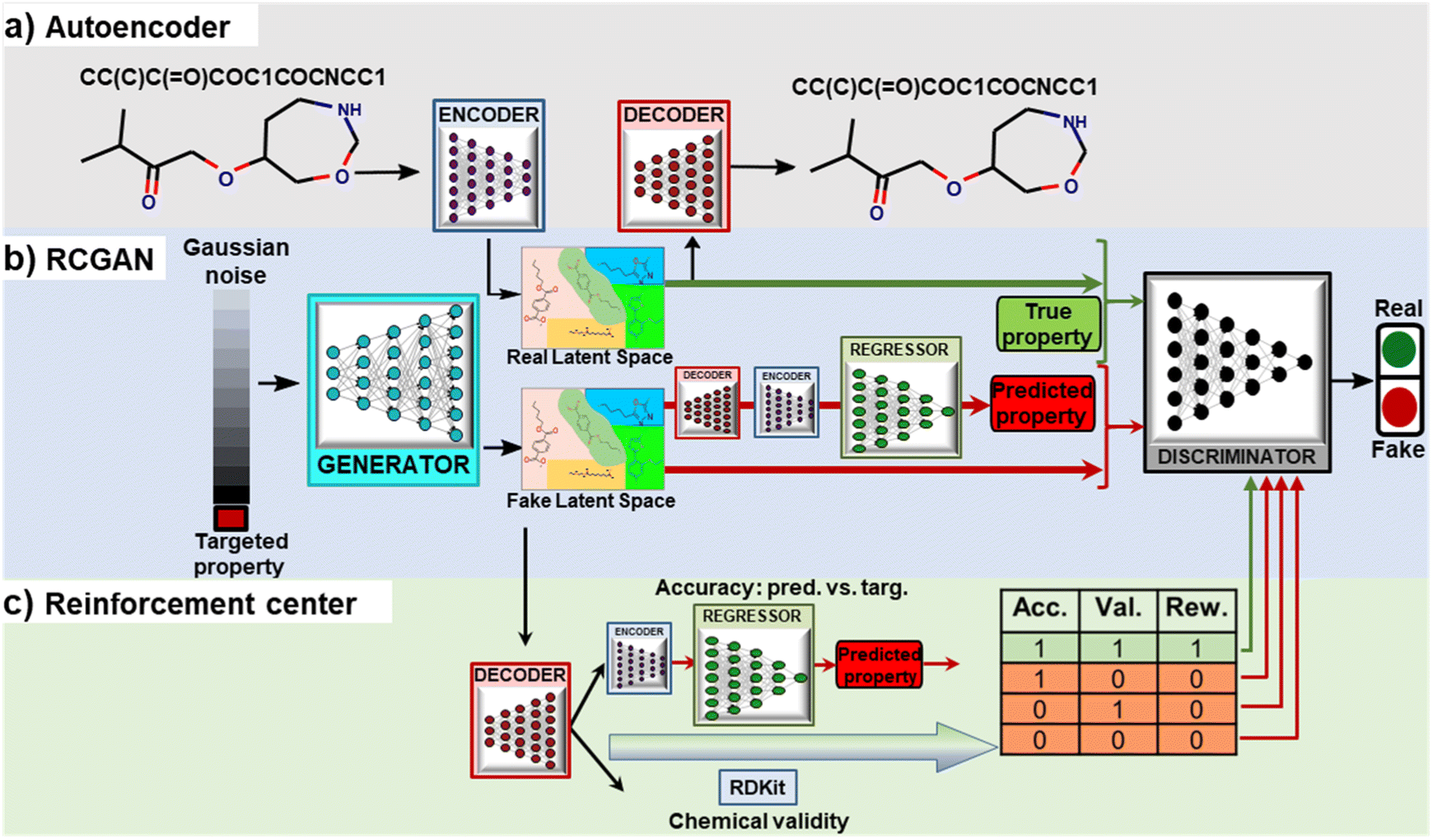Fig. 1 Architecture of the proposed RRCGAN for inverse molecule design with targeted ΔE_H–L. (a) AE architecture for converting discrete molecule representations to and from a continuous latent space. (b) RCGAN architecture. The generator takes targeted property and Gaussian noise as inputs to generate latent vectors. The discriminator distinguishes the synthesized molecules from the real ones based on their latent vectors and their assigned ΔE_H–L. The regressor predicts the property values from the generated latent vectors. (c) Scheme of the reinforcement center that biases the discriminator towards generation of the valid and accurate molecules.

In this work, RCGAN has a generator, a discriminator, and a regressor network. RCGAN learns the hidden relationship between the latent vectors and properties of the training molecules for generating new latent vectors conditioned on targeted ΔE_H–L (continuous labels), which are then converted to the SMILES strings using the decoder (Fig. 1b). The regressor is modified from Google Inception V2 (ref. 37) (Fig. S4†). It is built as a quantitative structure–activity relationship (QSPR) model for predicting ΔE_H–L. To generate a latent vector conditioned on a ΔE_H–L value, the generator receives a concatenated vector (129 × 1) consisting of a targeted ΔE_H–L and a randomly generated noise vector z in a 128 × 1 matrix (Fig. S5†). In contrast to the RNN-based models that generate one token at a time based on previously generated tokens,^18,19 our generator employs a CNN architecture which can generate the latent vectors in a single step. The generated latent vector has a dimension of 6 × 6 × 2 and is expected to contain chemical information hidden in the high-dimensional training data. The discriminator is trained by comparing the input concatenated vectors for both training and generated molecules (Fig. S6†). The trained decoder is used to convert the synthesized latent vectors to SMILES that are then fed into the trained encoder to generate the latent vectors, which serve as the input to the regressor. The regressor then predicts ΔE_H–L that corresponds to the generated latent vectors. If the regressor is directly fed with the output of the generator, it has an R² of 0.80 and MAE of 0.60 eV (comparing the true and predicted values), which are lower than the ones (R² of 0.90 and MAE of 0.45 eV) afforded by the regressor fed with the converted latent vectors. The discriminator performs two functions. First, it determines whether the concatenated vector is from a real (training) molecule or a fake (generated or synthesized) one by comparing the statistical distribution of the two. Second, it tells whether a generated molecule corresponds to the targeted ΔE_H–L value.

Finally, a reinforcement center is included in the RRCGAN framework to ensure that the generated molecules are chemically valid and accurate in comparison of the validated ΔE_H–L with the targeted ΔE_H–L (Fig. 1c). First, the latent vectors generated by the generator are converted to the SMILES by the decoder and then fed into RDKit³⁸ to ensure that the SMILES are chemically valid. If a SMILES is valid, then “1” is assigned to the string; otherwise, “0” is assigned. Subsequently, a relative error (RE) of a targeted ΔE_H–L compared with the predicted value from the regressor is evaluated. If RE is less than 20%, “1” is assigned to represent an accurate sample. Only a latent vector with assigned numbers of both “1” (valid and accurate molecule) is labeled as a real sample. Otherwise, it is labeled as a fake one. These two constraints reinforce the discriminator to consider the molecules with both high chemical validity and high accuracy as the real molecules and others as the fake ones. In the training process, before the reinforcement center is activated, the generator and the discriminator are trained in a few epochs. Details about the architectures of these networks and their training processes are described in ESI note 2.† Their loss functions and training processes are described as follows.

2.1.2 Loss functions of encoder, decoder, regressor, generator, and discriminator. The loss function (L_AE) of AE is the sum of the cross entropy (L_AE1 for discrete one-hot encoded SMILES strings) and the mean square error (MSE) (L_AE2 for continuous property labels), as shown in the following equations.

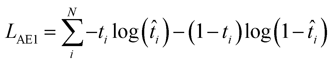
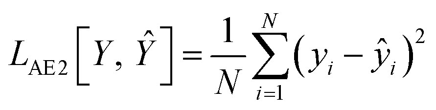
L_AE = L_AE1 + L_AE2 (1)

In eqn (2), t is the true value (either 0 or 1) showing binary categories in the one-hot encoding vectors used for each SMILES. The predicted t̂ can be any value between zero and one, while they must sum to 1 in the last SoftMax layer of the decoder. In eqn (3), ŷ is the predicted ΔE_H–L, y is the true ΔE_H–L, and N is the number of molecules. The decoder is conditioned on the known ΔE_H–L to improve the accuracy of the decoder. Eqn (3) is to calculate the mismatch between the predicted ΔE_H–L from the decoder and the true ΔE_H–L. The predicted ΔE_H–L from the decoder, however, is not used in the model as it has a lower accuracy compared to the regressor.

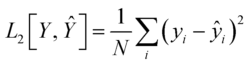
The loss function of the regressor is defined as the L₂ in eqn (4). It measures the difference between the predicted and true ΔE_H–L.

Loss_R = L₂[Y, R(Z)] (4)

where Z is a latent vector output from the encoder and Y is the true ΔE_H–L. L₂ is defined in eqn (5).where y is the targeted ΔE_H–L value, ŷ is the predicted ΔE_H–L value from the regressor or R(Z), and N is the number of molecules.

As shown in eqn (6), the loss function of the generator includes two terms. The first one is the same as the loss for the least square GAN (LSGAN),³⁹ while the second one is the regularized loss for the regressor.

where is the expectation function, the subscript (z–P_z(z)) shows the synthesized molecules from the generator, and z is a random noise and the input of the generator. D₂ and E are the decoder and encoder, respectively. D is the discriminator that uses the latent vectors generated from the generator and the predicted ΔE_H–L from the regressor to classify them into two groups of the fake [0] or real [1] molecules. When feeding the regressor with the generated molecules, the L₂ loss is calculated and then used as the regularization term in the loss function of the generator. w is the weight parameter for the regularization term. The combined loss function ensures that the generator and discriminator are simultaneously trained to avoid mode collapse.

The loss function of the discriminator is the same as the one used for LSGAN (eqn (7)).³⁹

where E is the encoder and E(X) is the latent vector output from the encoder. In the pre-training process, when the reinforcement has not been activated, the subscript X–P_data(X) indicates that the molecule is sampled from the training data, and z–P_z(z) refers to all the generated molecules by the generator. After 5 epochs of initial training of the generator and discriminator, the generator generates 1000 molecules that are evaluated for validity and accuracy by the reinforcement center. X–P_data(X) refers to the generated molecules that are chemically valid and have the predicted ΔE_H–L with RE of <20%, and z–P_z(z) refers to the generated molecules that do not pass either of the validity or accuracy tests.

2.1.3 Training of RRCGAN. The process starts with training the AE and the regressor using ∼132 K molecules from the PubChemQC database.^34,35 We considered ΔE_H–L as the property of interest. The AE was trained by minimizing the discrepancy between the input SMILES strings to the encoder and the output ones from the decoder. Fig. S7† shows that the loss of AE is stabilized after 1000 epochs. The latent vectors have dimensions of 6 × 6 × 2. Evaluation of the decoder's performance was done by comparing the true one-hot encoded SMILES strings with those generated by the decoder. Our findings indicate that 87% of the SMILES strings (from the testing molecules) were accurately converted back to the original input ones. Also, 90% of the converted SMILES strings corresponded to the chemically valid molecules. To assess the fidelity of the reconstruction, we also calculated categorical accuracy, which measures the percentage of correctly reconstructed characters in the output SMILES strings. Our AE achieved a categorical accuracy of 98.6%, slightly surpassing the value of 98.5% reported by Gómez-Bombarelli et al.² Fig. S8† shows three randomly selected one-hot encoded SMILES strings from the testing and training datasets as well as their respective conversions by the decoder. We also explored alternative latent vectors with dimensions of 4 × 4 × 2 and 8 × 8 × 2. The 4 × 4 × 2 latent vectors were found to be insufficient in capturing necessary information for the decoder to accurately reconstruct the input SMILE strings. The 8 × 8 × 2 latent vectors yielded a comparable accuracy of 86% in converting the SMILES strings. But as shown in Fig. S9,† the model trained with the 8 × 8 × 2 latent vectors has a reduced R² of 0.3 compared to an R² of 0.7 from the model trained with the 6 × 6 × 2 vectors.

The latent vectors outputted from the pre-trained encoder, along with the corresponding ΔE_H–L were used to train the regressor. Fig. S10† shows that the loss of the regressor is stabilized after 150 epochs. As shown in Fig. S11,† the regressor affords a coefficient of determination, R-squared (R²) of 0.98, and a mean-absolute-error (MAE) of 0.19 eV for training and R² of 0.95 and MAE of 0.33 eV for testing. Table S1† provides a comparison of the regressor's accuracy with other models. The pre-trained regressor is used to predict ΔE_H–L of the synthesized molecules from the generator. It is also used in the reinforcement center to screen out the molecules with the unsatisfactory ΔE_H–L accuracy.

After the AE and the regressor are pre-trained, the generator and discriminator are first trained for 5 epochs. After that, the reinforcement center is activated. Then, the generator generates 1000 latent vectors in response to the input ΔE_H–L values. The reinforcement center groups the molecules based on two criteria: the SMILES validity and accuracy of the predicted ΔE_H–L values compared to the targeted ones. To check the validity of the generated molecules, their latent vectors are first converted to SMILES by the decoder and then validated by RDKit. Meanwhile, these SMILES are converted to the latent features and then fed to the pre-trained regressor for predicting ΔE_H–L. The reinforcement center selects the generated molecules that are chemically valid and have the predicted ΔE_H–L within RE of 20% of the targeted values. These selected molecules are labeled as “1” and the remaining ones are labeled as “0”. Then, these grouped molecules are fed to train the discriminator. The loss evolution of the generator and discriminator is represented in Fig. S12.† It shows that after the reinforcement center is activated, the loss of the generator is fast reduced and stabilized after 150 epochs. The low and stabilized losses of both the generator and discriminator indicate a successful model training. We conducted a control experiment by disabling the reinforcement center in the training process. As shown in Fig. S13,† the losses of the generator and the discriminator without the reinforcement center do not converge after 200 epochs. Hyperparameters for these trained networks are shown in Table S2.† Evaluation metrics such as R², mean absolute error (MAE), RMSE, MSE, and RE are defined in eqn (S1)–(S5) (ESI note 3†).

2.2 Evaluation of RRCGAN

Performance of RRCGAN was evaluated by comparing the DFT-calculated ΔE_H–L of the generated molecules with the targeted ΔE_H–L and the predicted ΔE_H–L by the regressor, respectively. ΔE_H–L values of the molecules that were used to train the initial model were in the range of 1.05–10.99 eV. A set of 630 molecules was generated, as outlined in the methodology section. The predicted ΔE_H–L values by the regressor were first compared with the DFT calculated ones for the 630 evaluated molecules (Fig. 2a). Their R² and MAE were calculated to be 0.87 and 0.5 eV, respectively. This high prediction accuracy suggests that the regressor catches the hidden chemical rules to correlate the molecule structures with ΔE_H–L. Fig. 2b shows RE distribution of the predicted ΔE_H–L by the regressor compared with the DFT calculated ones. 91% of the molecules show within 20% RE of the DFT-calculated values. The results shown in Fig. 2a and b suggest a high accuracy of the regressor in predicting ΔE_H–L of the generated molecules. Thus, it is acceptable to use the regressor for screening the generated molecules for saving time and cost from using the DFT calculation. In addition, the targeted ΔE_H–L and DFT-evaluated ΔE_H–L of the generated molecules were compared to evaluate the accuracy of the RRCGAN model in generating the molecules (Fig. 2c). The data shows R² and MAE of 0.62 and 1.0 eV, respectively. Distribution of RE between the DFT-calculated and targeted ΔE_H–L is shown in Fig. 2d. ∼75% of the molecules have ΔE_H–L calculated by DFT within 20% RE of the targeted values, showing an acceptable accuracy in such a de novo molecule generation task in this large range of targeted values. The importance of this one-to-one comparison lies in its ability to showcase the model's efficacy and precision on targeting the property values. Compared to some state-of-art molecule generation models as shown in Table S3,† our model shows uniqueness in realizing this important goal. In addition, it is superior to them in terms of realizing targeted, extrapolative generation of molecules with higher or comparable accuracy at the same time. In a separate experiment, we targeted a single value to generate ∼2500 valid molecules. Fig. S14† shows the distribution of the predicted values for the ∼2500 generated molecules corresponding to a targeted ΔE_H–L value of 8.29 eV. It shows that 85% of the generated molecules have a predicted ΔE_H–L value within 20% RE of the targeted one. An obvious disadvantage of the string-based representation methods, e.g., SMILES, is that information about the bond lengths and 3D configurations is lost. Trained with the molecules presented by them, the model shows a limitation in accuracy. A better accuracy may require more input information like the molecules' 3D configurations,⁴⁰ while it is a trade-off with the computational cost. In future, a distance geometry method⁴¹ can be used to embed some 3D information into the SMILES to validate if the accuracy of RRCGAN can be improved.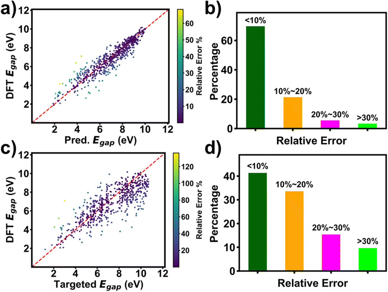

Fig. 2 Comparison of the targeted, predicted, and DFT calculated ΔE_H–L values of the randomly sampled 630 molecules among all the generated ones. (a) Predicted versus DFT calculated ΔE_H–L colored with RE of those values; (b) distribution of RE of the predicted and DFT calculated ΔE_H–L; (c) targeted versus DFT calculated ΔE_H–L colored with RE of those values; and (d) distribution of RE of the targeted and DFT calculated ΔE_H–L.

2.3 Transfer learning for biasing ΔE_H–L towards higher values

Table S4† shows statistics of the initial training molecules. Among the 132 K molecules, only 461 exhibited a ΔE_H–L value of ≥10 eV. Although the initial RRCGAN model occasionally generates outlier molecules with ΔE_H–L of ≥10 eV, among the 630 molecules shown in Fig. 2, there are only three with ΔE_H–L of 10.0, 10.10, and 10.15 eV. Importantly, none of these values exceeded the range of the original training dataset, which spanned from 1.05 to 10.99 eV, which is expected for an interpolation model. To train a new model for biasing the generation toward ΔE_H–L of >10.99 eV, the number of these molecules is not sufficient. In contrast, transfer learning has shown a great promise in solving the data scarcity problem.^24,42 “Transfer learning” refers to the process of transferring knowledge from an already trained model to a new one, thereby enhancing the accuracy of the latter even when trained with limited data.⁴³ Thus, to bias ΔE_H–L towards higher values for extrapolating the property space, a transferred model was trained via fine-tuning the initial RRCGAN on the new molecules with increased ΔE_H–L values.

The workflow of such an iterative generative algorithm is shown in Fig. 3a. As a demo, herein, only two iterations were investigated. In the first iteration, a set of 1000 molecules with ΔE_H–L values of ≥10.0 eV was used for training. Out of those, 461 molecules with ΔE_H–L values of ≥10.0 eV were sourced from the PubChemQC database (Fig. 3a(ii) and Table S5†), while the remaining molecules were newly generated by the model. To generate them, we employed a multiple batch generation process, each consisting of 50 targeted ΔE_H–L values uniformly sampled within the range of 8–11 eV. Subsequently, we screened the generated molecules corresponding to these targeted ΔE_H–L values using the regressor model, selecting those with the predicted ΔE_H–L value greater than 9.5 eV. These molecules were then subjected to DFT calculations for validation, and only those with DFT-calculated ΔE_H–L values of ≥10 eV were finally selected. This batch generation process was repeated using different sampled targeted values until 539 valid, unique, and novel molecules with the DFT-validated ΔE_H–L values of ≥10 eV were obtained. In the second iteration, the transferred model was fine-tuned using the generated molecules with validated ΔE_H–L of ≥10.2 eV from the first transferred RRCGAN model. Fig. 3b shows the distributions of ∼132 K initial molecules used for training the initial RRCGAN model and the generated molecules in different transfer learning iterations. The ΔE_H–L values of the generated molecules by the initial model are in the 2–10.15 eV range with a mean ΔE_H–L of 6.33 eV, which is close to 5.94 eV, the average of the original training molecules. Only 0.5% of the outlier molecules have ΔE_H–L of ≥10 eV. After the first iteration, the transferred model generates the molecules with a mean ΔE_H–L of 7.4 eV and a maximum ΔE_H–L of 11.6 eV. The percentage of the molecules with ΔE_H–L of ≥10 eV increases to 5%. After the 2nd iteration, the generated molecules have a mean ΔE_H–L of 8.7 eV and a maximum ΔE_H–L of 12.9 eV. The percentage of the molecules with the predicted ΔE_H–L of ≥10 eV increases to 16%. These results illustrate that the iterative transfer learning can push the generation toward higher ΔE_H–L values and increase maximum ΔE_H–L.

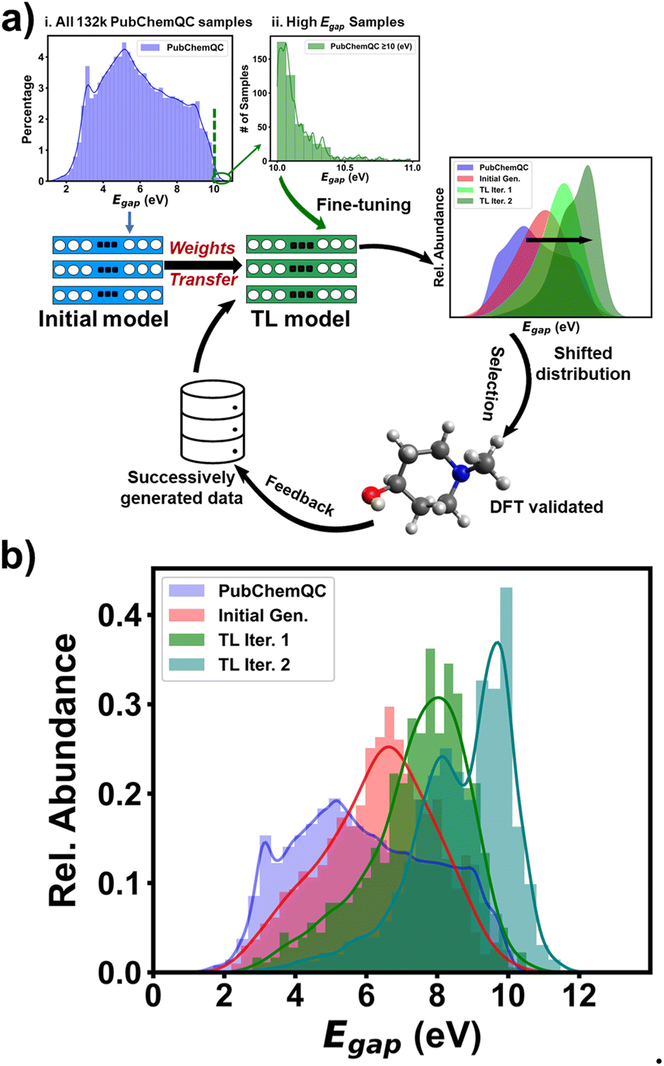Fig. 3 Workflow of iterative transfer learning and model performance. (a) Schematic of the iterative transfer learning for generating molecules with targeted ΔE_H–L beyond the range of initial training data. (b) ΔE_H–L distributions of the initial training molecules in the PubChemQC database, the molecules generated by the initial RRCGAN model, and the molecules generated by the 1st transferred model and the 2nd transferred model.

The application of transfer learning in molecule design has been explored in other studies as well.^44,45 However, our approach distinguishes itself from the method proposed by Merk et al.⁴⁴ in terms of our fine-tuning strategy. While they utilized historical data featuring high experimental activities, we employed newly generated molecules as training samples. This unique approach led us to uncover a previously unexplored functional group (C–F) that exhibits a strong correlation with high ΔE_H–L values. The fine-tuning process using these newly generated molecules yielded a pronounced emphasis on exploration over exploitation. Furthermore, our framework differs from the work introduced by Korshunova et al.⁴⁵ Although they also employed newly generated samples for fine-tuning, their framework lacks the capability to target multiple values within the high-value region. In contrast, with sufficient fine-tuning, our framework has the potential to precisely target a range of values within the explored high-value region.

2.4 Analysis on the generated molecules

2.4.1 Analysis of structural features of molecules. The active search strategy outlined earlier enables the generation of the molecules with the ΔE_H–L values higher than those found in the original training dataset. It can be deduced that RRCGAN has successfully learned the chemical rules contained in the SMILES strings to establish the structure–property relationship. Herein, the structures of the generated molecules are analyzed to understand how the model captures the chemical insights. Fig. 4 displays 20 representative molecules with the DFT-calculated ΔE_H–L values ranging from 2.38 to 13.07 eV and have RE within 10% of the targeted values. Fig. 4a showcases molecules with the ΔE_H–L values of <6.5 eV, while Fig. 4b presents those with the ΔE_H–L values of >6.5 eV.

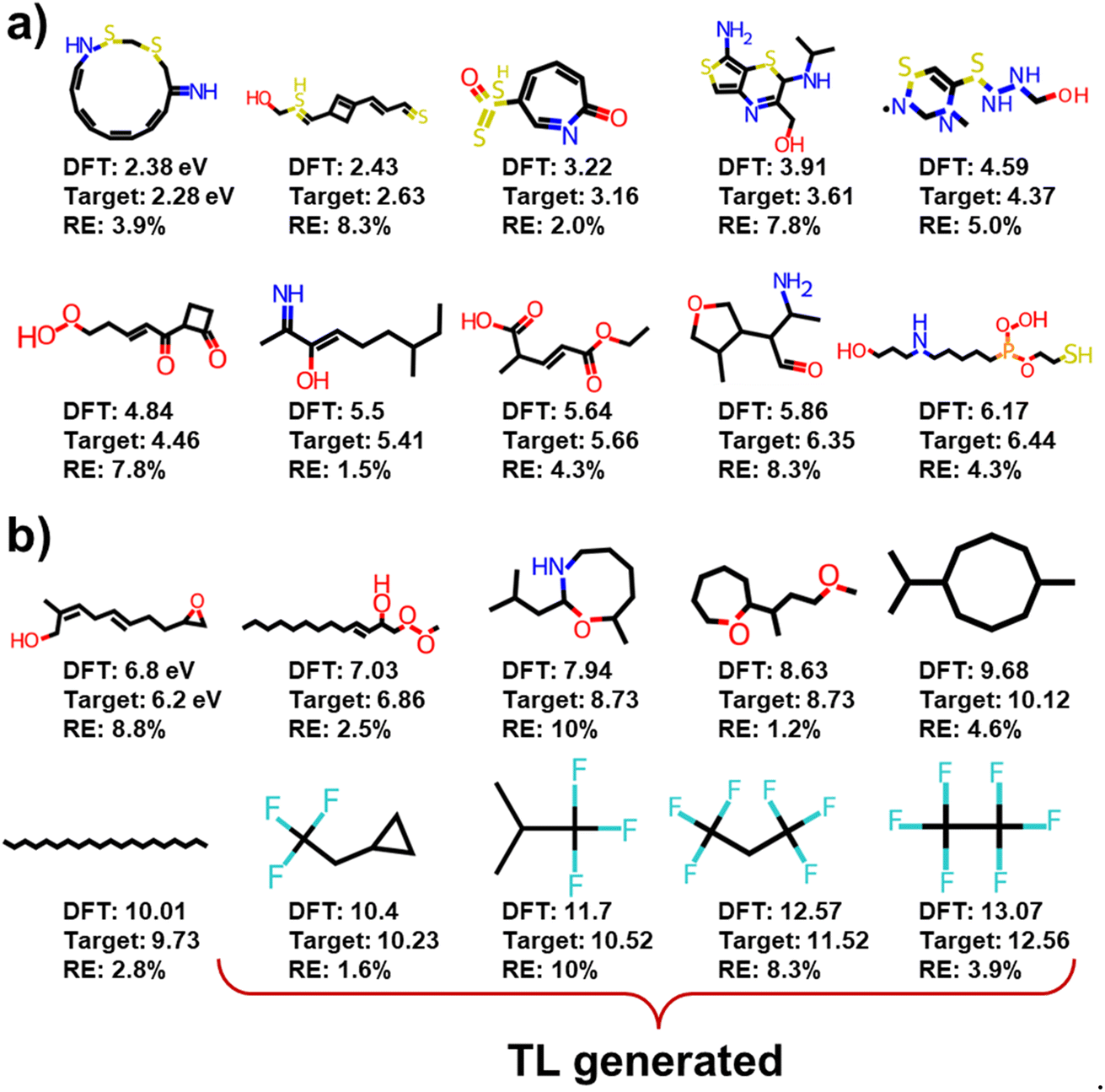Fig. 4 Representative examples of molecules generated by the original and transferred RRCGAN models: the molecules with (a) ΔE_H–L of <6.5 (eV), and (b) ΔE_H–L of >6.5 (eV).

Comparison of the molecules with high and low ΔE_H–L values highlights several key observations. The molecules featuring alternated single and multiple bonds – which are referred to as conjugated systems, unsaturated rings, and radical electrons, tend to exhibit lower ΔE_H–L values. Conversely, the molecules with linear structures which are characterized by single bonds or saturated rings tend to display higher ΔE_H–L values. Moreover, the presence of sulfur (S) and nitrogen (N) decreases ΔE_H–L. This effect can be attributed to the increased extent of orbital overlap facilitated by these elements, ultimately reducing ΔE_H–L.⁴⁶

In addition to the structure–property relationship disclosed from the initial RRCGAN model, the transferred model reveals a different but noteworthy correlation. That is the presence of fluorine (F) atoms bonded to carbon (C) atoms in the molecules increasing ΔE_H–L. That could be because F is the most electronegative element in the periodic table. In a molecule, F exerts a strong electron-withdrawing effect, which raises the LUMO level to get a higher ΔE_H–L.⁴⁷ But this rule remains undisclosed by the initial model due to the scarcity of the F-containing molecules in the initial training dataset. Among the 132 K initial training molecules, only 4 molecules contain the F atom and have ΔE_H–L of >10 eV. As depicted in Fig. 4b, the generated molecules by the transferred model have ΔE_H–L of 13.07 eV. They all include the F–C bonds. This observation illustrates the effectiveness of the transferred model in learning a critical structural feature even present in the limited samples when doing the extrapolative generation. Meanwhile, they all include the single bond and saturated rings. This knowledge is transferred from the initial model that these two features tend to improve the ΔE_H–L values. These observations confirm that the model can effectively correlate the structures with the properties, aligning with the established chemical rules.^47,48 The strong agreement between the model's predictions and established chemical principles enhances confidence in the utilization of this deep generative model for the efficient and cost-effective generation of novel molecules with desired properties. Adding objectives related to synthetic accessibility for generated molecules is a thoughtful approach to enhance the practical utility of the proposed generative model. This could include criteria such as the complexity of the chemical structure, the presence of synthetically challenging motifs, or adherence to established synthetic rules.⁴⁹ Additionally, involving domain experts in the development and validation process can significantly enhance the effectiveness of the synthetic accessibility objectives in the proposed generative model.

Visualizing these representative molecules in Fig. 4 affords a qualitative correlation of the structures with their ΔE_H–L. To establish a quantitative relationship, we trained an XGBoost regression model which takes 18 structural features (ESI note 4†) as input to predict ΔE_H–L. From the feature importance analysis (Fig. S15†), we picked four important structural features that most affect the prediction. They are the number of the saturated rings, number of the hydrogen-bond acceptors, the heavy atoms molecular weight, and number of the rotatable bonds. A saturated ring is defined as a cycle composed solely of single bonds, while an aromatic ring consists of alternating single and double bonds, as exemplified by benzene. The hydrogen-bond acceptors are typically electronegative atoms with lone pairs of electrons, such as oxygen (O), nitrogen (N), and sometimes sulfur (S). The rotatable bonds are non-ring single bonds connected to non-hydrogen, non-terminal atoms. Amid C–N bonds are excluded due to their high rotation barriers.⁵⁰ In Fig. 5, we present the percentage distribution of these selected features presented within both the training and generated molecules. Feature distributions of the generated molecules are slightly different from those of the training ones, demonstrating the generator's capability in exploring the new design space to generate the molecules with the targeted ΔE_H–L. Specifically, Fig. 5a reveals a higher percentage of the generated molecules with a single saturated ring compared to the training molecules. Fig. 5b illustrates a decrease in the occurrence of the generated molecules with 2 and 3 hydrogen bond acceptors, while the number of the molecules with higher hydrogen-bond acceptors is increased. Moreover, the heavy atom molecular weights tend to increase ΔE_H–L (Fig. 5c), indicating a tendency for the model to generate larger molecules in request of higher ΔE_H–L. Additionally, Fig. 5d indicates that the number of the rotatable bonds increases in correspondence of the higher ΔE_H–L values. It is worth noting that these structural features were not directly used as descriptors for the RRCGAN model. It is likely that such information is implicitly captured within the latent vectors. Furthermore, Fig. S16† presents the ranking of other features which are also associated with ΔE_H–L. Further explanations and details regarding these features can be found in ESI note 4.†

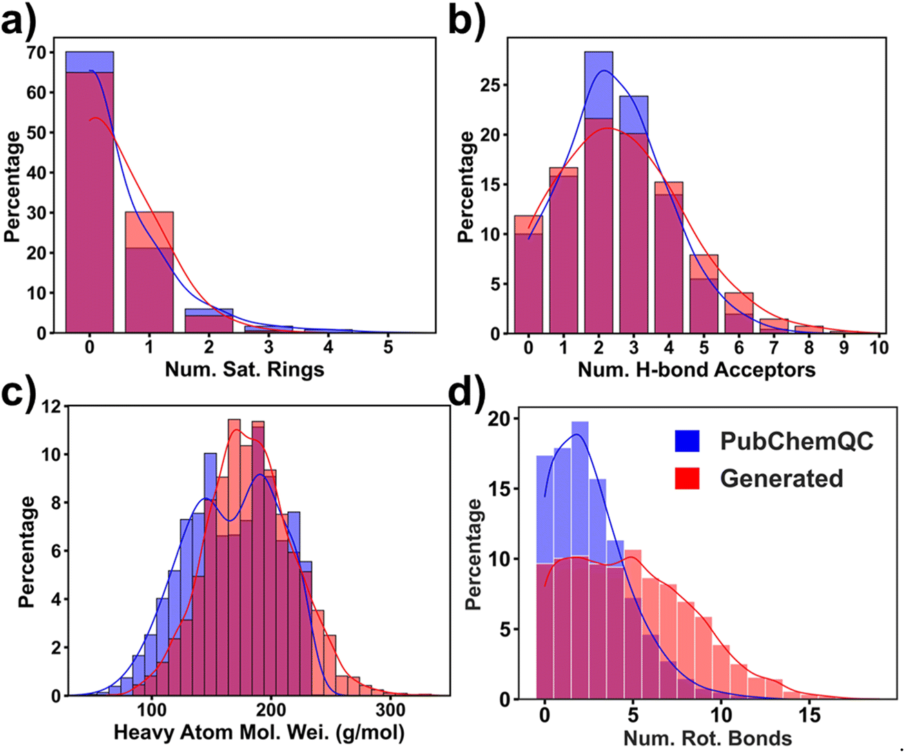Fig. 5 Density distribution of the four selected features for the training and generated molecules: (a) number of saturated rings; (b) number of aromatic rings; (c) molecular weight of the heavy atoms; (d) number of rotatable bonds.

2.4.2 Dimension reduction on the latent vectors of the molecules. The latent vectors, which are the output of the encoder, were used as the input for training the RRCGAN model. These continuous vectors can connect the discrete SMILES representations with their hidden structural information for generating the molecules responding to their targeted properties. They are, however, high-dimensional and are difficult to interpret. We hypothesize that if they can be mapped to a lower dimensional space, the molecules that share similar structural features would be clustered together in the plots, and the generated molecules would follow a similar pattern to that of the training ones.

To validate the hypothesis, we applied t-distributed stochastic neighbor embedding (t-SNE), a non-linear dimension reduction method, to project the latent vectors of both training and generated molecules (Fig. 6). First, we divided ΔE_H–L into four ranges. The ranges for the training molecules are ≤4.4 eV, [4.4–5.7 eV], [5.7–7.5 eV], and >7.5 eV. The ranges for the generated molecules are ≤4.5 eV, [4.5–5.9 eV], [5.9–7.7 eV], and >7.7 eV. Each range was calculated by quantiles to have the same number of molecules. The projected latent vectors were then colored based on their ΔE_H–L ranges, where the dark blue and dark red colors represent the low and high values, respectively. As shown in Fig. 6, the first component of t-SNE (t-SNE1) separates the molecules based on their ΔE_H–L values. The molecules in the same ΔE_H–L range are clustered into close regions in the plots. Molecules with ΔE_H–L > 6 eV are in a region with t-SNE1 < 0 and vice versa. In Fig. 6a and b, molecule (7) is a representative sample with ΔE_H–L of ≤4.4 eV and ≤4.5 eV for the training and generated molecules, respectively. Molecules (3) and (4) represent the ones with ΔE_H–L of >7.5 eV and >7.7 eV for the training and generated molecules, respectively. Linear molecules with single bonds and fewer sulfur and nitrogen atoms are grouped in the high ΔE_H–L value region, while molecules with rings, conjugated systems, and more sulfur and nitrogen atoms occupy the low ΔE_H–L value regions. These results agree well with the observations from Fig. 4. Moreover, the generated molecules are clustered in the same regions as the ones for the training molecules (Fig. S17†), further validating that the generator has successfully learned the structural information from the latent vectors of the training molecules for generating novel molecules with the targeted ΔE_H–L. As a comparison, we also performed a principal component analysis (PCA) and a spectral embedding analysis on the same molecules used for the t-SNE analysis. The results are shown in Fig. S18.† Discussion on the PCA and spectral embedding results is described in ESI note 5.† In conclusion, it is found that t-SNE outperforms the other two methods for data visualization in this case.

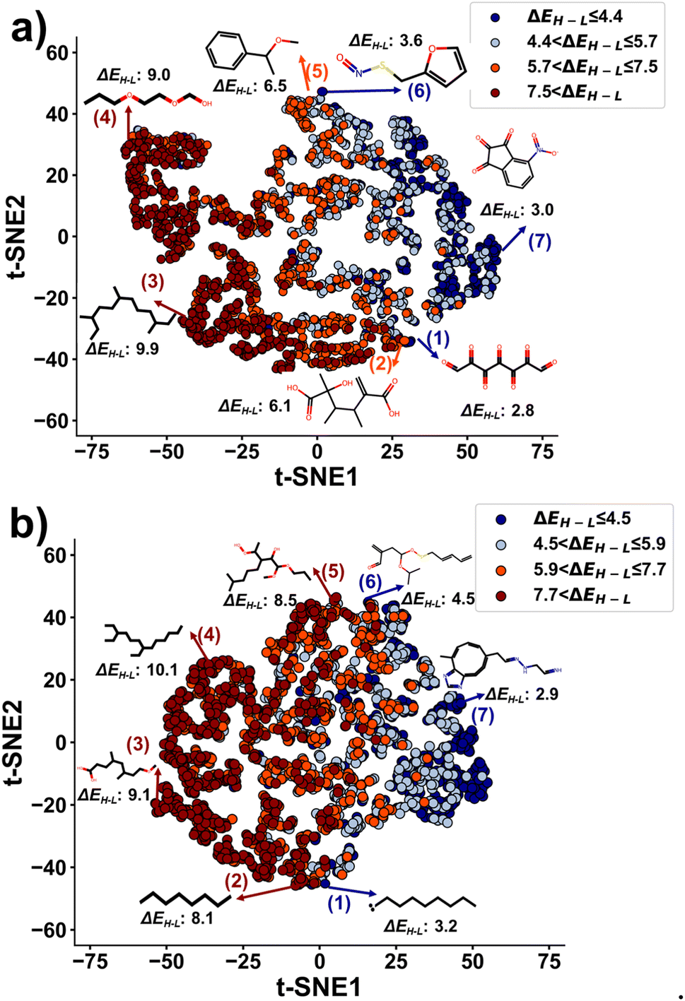Fig. 6 t-SNE plots of the latent vectors of the training and generated molecules output from the encoder: (a) training molecules; (b) generated molecules. Unit of ΔE_H–L is eV.

We have also presented some molecules in the boundaries between the two gap ranges of the highest and lowest ΔE_H–L to show the similarities of the structures although they are in the two different ranges. When comparing molecules (1) and (2) in Fig. 6a, the existence of a conjugated system in molecule (1) lowers ΔE_H–L, which agrees well with the conclusion shown in Fig. 4. When comparing molecules (1) and (2) in Fig. 6b, the existence of radical electrons in molecule (1) lowers ΔE_H–L. When compared to molecule (5), molecule (6) has the sulfur atom, thus reducing the ΔE_H–L value (Fig. 6a and b). For such molecules with close structures but different ΔE_H–L values, the reduced latent space is not enough to distinguish them.

3. Conclusion

In this study, we designed and implemented a deep generative framework named RRCGAN for de novo design of molecules toward biased ΔE_H–L values. To develop the model, we first trained the encoder and decoder. Subsequently, the encoded latent features of the molecules were fed to the regressor to predict ΔE_H–L, which enables the GAN to generate the molecules that meet the desired values while remaining chemically valid. It is worth mentioning that only SMILES strings are used as the input of the model, and no other complicated chemical descriptors are employed in the study. ΔE_H–L of the generated molecules are validated by DFT and compared with the targeted values. The developed RRCGAN is transferred by using the limited, generated molecules in the previous iteration for the next-iteration molecule generation toward ΔE_H–L values beyond those in the initial training data. In just two iterations, the generated molecules exhibit an increased mean ΔE_H–L of 10.5 eV compared to mean ΔE_H–L of 5.94 eV in the PubChemQC database.

To ensure the reliability and efficacy of the model, the structures and the latent features of both training and generated molecules were qualitatively and quantitatively analyzed. The analyses reveal that the model has successfully captured the underlying structure–property relationship, which agrees well with the established physical and chemical rules. The model then correlates the structural features with the values of ΔE_H–L for generating novel molecules with targeted ΔE_H–L. The proposed RRCGAN framework would afford a trustworthy, purely data-driven methodology for the highly efficient generation of novel molecules without the need for physical or chemical inputs.

4. Methods

4.1 Data collection and curation

We used ∼132 K out of 3 million molecules from the PubChemQC database,³⁵ for training the original RRCGAN model. More details of preparing the 132 K training molecules are provided in ESI note 6.† PubChemQC is a quantum chemistry database with molecules from the PubChem Project.⁵¹ We split the molecules into training and testing datasets for training the AE and regressor as shown in Fig. S19.† Using RDKit, canonical SMILES were extracted to represent the molecules.⁵² To one-hot encode SMILES, a subset of 27 different characters was used as shown in Fig. S1.† We considered 40 as the maximum number of characters in each SMILES. With padding for sequences with less than 40 characters, a fixed one-hot encoded matrix size of 40 × 27 was used. The training molecules have up to 20 heavy atoms of C, O, N, S, P, and F. We reserved the last character as the closing character. As a result, the generated molecules can have up to 39 heavy atoms. These SMILES representations were split into training, validation, and test datasets in a ratio of 6 : 2 : 2. The training and validation datasets were used to finetune the hyperparameters of the encoder, decoder, and regressor, while the test datasets were used to evaluate the final performance of the model. The ΔE_H–L values in the range of 0–15 eV were normalized to 0–1.0 for the model development.

4.2 Batch generation

For generating 630 molecules shown in Fig. 2, we used a batch of 70 targeted values that were sampled uniformly in the range of 1–11 eV. We then repeated each of these sampled targeted values 10 times to generate 700 molecules in one batch. We generated 10 batches with different seeds of random sampling that results in a total of 7000 generated molecules. Please note that by changing the number of targeted values and repetition times the number of molecules in one batch can be varied. The directory “model_regular” from the GitHub repository includes the file related to batch generation. The Jupyter Notebook file named “Main_model_batchgen.ipynb” contains the code for batch generation. We analyzed the generated molecules regarding their validity, uniqueness, and novelty. Using RDKit, we checked atoms' valence and consistency of bonds in the aromatic rings for the validity calculation. Novelty is indicated by the fraction of the generated molecules that are not present in the PubChemQC database. Uniqueness is defined as the ratio of molecules that are distinguished from each other in the same batch. In the example of generating 7000 molecules, 11% were valid of which 95% were unique. Also, 94% of these valid and unique molecules were novel compared to the training molecules in the PubChemQC database. The resulting 650 valid, unique, and novel molecules were then calculated by density functional theory (DFT), and 630 of them were finished simulation within the set time limit of 8 hours. The DFT output of the final samples are included in “analysis” directory of the GitHub repository. The transferred models in first and second iterations are also provided in “model_transfer” and “model_transfer2” folder of the published GitHub repository.

4.3 DFT calculation

We used Open Babel, an open chemical toolbox,^41,53 to convert the generated SMILES strings to 3D coordinates. Open Babel adds hydrogens to the molecules and generated their 3D coordinates. Then, a quick local optimization was carried out in 50 steps by the MMFF94 force field. The DFT calculations for all molecules were carried out using Gaussian 16.C.01. Geometry optimization and frequency calculations were carried out using the B3LYP (VWN3) functional^54–56 with the split-valence, double-zeta, and polarized basis 6-31G(2df,p). Restricted closed-shell calculations were performed for all molecules. ΔE_H–L values, the energy difference between HOMO and LUMO eigenvalues, were extracted from the DFT results. To ensure that the calculation is accurate enough, we calculated ΔE_H–L of 59 molecules randomly selected from the PubChemQC database.³⁴ Among them, calculation of 46 molecules was finished within 8 hours. The calculated values were compared to the ones listed in the PubChemQC database. The result shows that they have a low MAE of 0.14 eV (Fig. S20†).

Data availability

The corresponding data and codes can be available at https://github.com/linresearchgroup/RRCGAN_Molecules_Ehl.

Author contributions

J. L. conceived the idea. D. L. developed the original framework which was significantly modified by K. S. K. S. performed the model training and data analysis. K. S. and J. L. wrote the complete manuscript. Y. X. assisted K. S. in writing the first draft. F. B. L. assisted in discussing the structural features of the molecules. B. K. and K. S. performed the DFT simulations. O. I. provided valuable discussion and contributed the writing about the analysis of the generated molecules. J. L. oversaw all research phases and provided guidance to the research team. All authors discussed and commented on the manuscript.

Conflicts of interest

The authors declare no competing financial interests.

Acknowledgements

J. L. thanks financial support by National Science Foundation (award number: 2154428) and U.S. Army Corps of Engineers, ERDC (grant number: W912HZ-21-2-0050). O. I. acknowledges the support from National Science Foundation (award number: 2154447). Part of the computation for this work was performed at the San Diego Supercomputer Center (SDSC) and the Pittsburgh Supercomputing Center (PSC) through allocation CHE200122 from the Advanced Cyberinfrastructure Coordination Ecosystem: Services & Support (ACCESS) program, which is supported by National Science Foundation grants #2138259, #2138286, #2138307, #2137603, and #2138296. Rest of the calculation was done on the high-performance computing infrastructure provided by Research Computing Support Services at the University of Missouri, Columbia MO, which is in part supported by National Science Foundation (Award number: CNS-1429294).

References

1. P. G. Polishchuk, T. I. Madzhidov and A. Varnek, J. Comput.-Aided Mol. Des., 2013, 27, 675–679.
2. R. Gómez-Bombarelli, J. N. Wei, D. Duvenaud, J. M. Hernández-Lobato, B. Sánchez-Lengeling, D. Sheberla, J. Aguilera-Iparraguirre, T. D. Hirzel, R. P. Adams and A. Aspuru-Guzik, ACS Cent. Sci., 2018, 4, 268–276.
3. Q. Yuan, A. Santana-Bonilla, M. A. Zwijnenburg and K. E. Jelfs, Nanoscale, 2020, 12, 6744–6758.
4. R. Gómez-Bombarelli, J. Aguilera-Iparraguirre, T. D. Hirzel, D. Duvenaud, D. Maclaurin, M. A. Blood-Forsythe, H. S. Chae, M. Einzinger, D.-G. Ha, T. Wu, G. Markopoulos, S. Jeon, H. Kang, H. Miyazaki, M. Numata, S. Kim, W. Huang, S. I. Hong, M. Baldo, R. P. Adams and A. Aspuru-Guzik, Nat. Mater., 2016, 15, 1120–1127.
5. J.-L. Reymond, Acc. Chem. Res., 2015, 48, 722–730.
6. J. Hachmann, R. Olivares-Amaya, S. Atahan-Evrenk, C. Amador-Bedolla, R. S. Sánchez-Carrera, A. Gold-Parker, L. Vogt, A. M. Brockway and A. Aspuru-Guzik, J. Phys. Chem. Lett., 2011, 2, 2241–2251.
7. J. Carrete, W. Li, N. Mingo, S. Wang and S. Curtarolo, Phys. Rev. X, 2014, 4, 011019.
8. D. Douguet, E. Thoreau and G. Grassy, J. Comput.-Aided Mol. Des., 2000, 14, 449–466.
9. Y. Dong, D. Li, C. Zhang, C. Wu, H. Wang, M. Xin, J. Cheng and J. Lin, Carbon, 2020, 169, 9–16.
10. K. Sattari, Y. Xie and J. Lin, Soft Matter, 2021, 17, 7607–7622.
11. H. Sahu, F. Yang, X. Ye, J. Ma, W. Fang and H. Ma, J. Mater. Chem. A, 2019, 7, 17480–17488.
12. X. Li, P. M. Maffettone, Y. Che, T. Liu, L. Chen and A. I. Cooper, Chem. Sci., 2021, 12, 10742–10754.
13. A. Tiihonen, S. J. Cox-Vazquez, Q. Liang, M. Ragab, Z. Ren, N. T. P. Hartono, Z. Liu, S. Sun, C. Zhou, N. C. Incandela, J. Limwongyut, A. S. Moreland, S. Jayavelu, G. C. Bazan and T. Buonassisi, J. Am. Chem. Soc., 2021, 143, 18917–18931.
14. D. P. Kingma, M. Welling, arXiv, 2013, preprint, arXiv:1312.6114v11,  DOI:10.48550/arXiv.1312.6114.
15. I. Goodfellow, J. Pouget-Abadie, M. Mirza, B. Xu, D. Warde-Farley, S. Ozair, A. Courville and Y. Bengio, Advances in Neural Information Processing Systems, 2014, vol. 27.
16. V. Mnih, K. Kavukcuoglu, D. Silver, A. Graves, I. Antonoglou, D. Wierstra, M. Riedmiller, arXiv, 2013, preprint, arXiv:1312.5602,  DOI:10.48550/arXiv.1312.5602.
17. K. Narasimhan, T. Kulkarni, R. Barzilay, arXiv, 2015, preprint, arXIv:1506.08941 DOI:10.48550/arXiv.1506.08941.
18. M. H. S. Segler, T. Kogej, C. Tyrchan and M. P. Waller, ACS Cent. Sci., 2018, 4, 120–131.
19. M. Popova, O. Isayev and A. Tropsha, Sci. Adv., 2018, 4, eaap7885.
20. B. Sanchez-Lengeling and A. Aspuru-Guzik, Science, 2018, 361, 360–365.
21. D. C. Elton, Z. Boukouvalas, M. D. Fuge and P. W. Chung, Mol. Syst. Des. Eng., 2019, 4, 828–849.
22. M. J. Kusner, B. Paige and J. M. Hernández-Lobato, arXiv, 2017, preprint, arXiv:1703.01925,  DOI:10.48550/arXiv.1703.01925.
23. N. C. Iovanac, R. MacKnight and B. M. Savoie, J. Phys. Chem. A, 2022, 126, 333–340.
24. N. C. Iovanac and B. M. Savoie, Mach. Learn.: Sci. Technol., 2020, 1, 045010.
25. Z. Zhou, S. Kearnes, L. Li, R. N. Zare and P. Riley, Sci. Rep., 2019, 9, 10752.
26. S. R. Atance, J. V. Diez, O. Engkvist, S. Olsson and R. Mercado, J. Chem. Inf. Model., 2022, 62, 4863–4872.
27. T. Pereira, M. Abbasi, B. Ribeiro and J. P. Arrais, J. Cheminf., 2021, 13, 21.
28. A. Gupta, A. T. Müller, B. J. H. Huisman, J. A. Fuchs, P. Schneider and G. Schneider, Mol. Inf., 2018, 37, 1700111.
29. Y. Xie, K. Sattari, C. Zhang and J. Lin, Prog. Mater. Sci., 2023, 132, 101043.
30. G. L. Guimaraes, B. Sanchez-Lengeling, C. Outeiral, P. L. C. Farias, A. Aspuru-Guzik, arXiv, 2017, preprint, arXiv:1705.10843,  DOI:10.48550/arXiv.1705.10843.
31. B. Sanchez-Lengeling, C. Outeiral, G. L. Guimaraes and A. Aspuru-Guzik, ChemRxiv, 2017, preprint,  DOI:10.26434/chemrxiv.5309668.v3.
32. S. H. Hong, S. Ryu, J. Lim and W. Y. Kim, J. Chem. Inf. Model., 2020, 60, 29–36.
33. B. Dou, Z. Zhu, E. Merkurjev, L. Ke, L. Chen, J. Jiang, Y. Zhu, J. Liu, B. Zhang and G.-W. Wei, Chem. Rev., 2023, 123, 8736–8780.
34. M. Nakata and T. Shimazaki, J. Chem. Inf. Model., 2017, 57, 1300–1308.
35. R. Ramakrishnan, P. O. Dral, M. Rupp and O. A. von Lilienfeld, Sci. Data, 2014, 1, 140022.
36. D. Weininger, J. Chem. Inf. Comput. Sci., 1988, 28, 31–36.
37. C. Szegedy, W. Liu, Y. Jia, P. Sermanet, S. Reed, D. Anguelov, D. Erhan, V. Vanhoucke, A. Rabinovich, arXiv 2015, preprint, arXiv:1409.4842,  DOI:10.48550/arXiv.1409.4842.
38. G. Landrum, Open-source Cheminformatics Software, https://www.rdkit.org, accessed 20 August 2023.
39. X. Mao, Q. Li, H. Xie, R. Y. K. Lau, Z. Wang and S. P. Smolley, arXiv, 2016, preprint, arXIv:1611.04076,  DOI:10.48550/arXiv.1611.04076.
40. N. W. A. Gebauer, M. Gastegger, S. S. P. Hessmann, K.-R. Müller and K. T. Schütt, Nat. Commun., 2022, 13, 973.
41. N. M. O'Boyle, M. Banck, C. A. James, C. Morley, T. Vandermeersch and G. R. Hutchison, J. Cheminf., 2011, 3, 33.
42. R. Zubatyuk, J. S. Smith, J. Leszczynski and O. Isayev, Sci. Adv., 2019, 5, eaav6490.
43. R. Yuan, Z. Liu, P. V. Balachandran, D. Xue, Y. Zhou, X. Ding, J. Sun, D. Xue and T. Lookman, Adv. Mater., 2018, 30, 1702884.
44. D. Merk, F. Grisoni, L. Friedrich and G. Schneider, Commun. Chem., 2018, 1, 68.
45. M. Korshunova, N. Huang, S. Capuzzi, D. S. Radchenko, O. Savych, Y. S. Moroz, C. I. Wells, T. M. Willson, A. Tropsha and O. Isayev, Commun. Chem., 2022, 5, 129.
46. M. Miar, A. Shiroudi, K. Pourshamsian, A. R. Oliaey and F. Hatamjafari, J. Chem. Res., 2021, 45, 147–158.
47. D. O'Hagan, Chem. Soc. Rev., 2008, 37, 308–319.
48. B. Wunderlich, Thermal Analysis of Polymeric Materials, Springer Science & Business Media, Berlin, Heidelberg, 2005.
49. P. Ertl and A. Schuffenhauer, J. Cheminf., 2009, 1, 8.
50. J. G. P. Wicker and R. I. Cooper, J. Chem. Inf. Model., 2016, 56, 2347–2352.
51. S. Kim, P. A. Thiessen, E. E. Bolton, J. Chen, G. Fu, A. Gindulyte, L. Han, J. He, S. He, B. A. Shoemaker, J. Wang, B. Yu, J. Zhang and S. H. Bryant, Nucleic Acids Res., 2015, 44, D1202–D1213.
52. N. M. O'Boyle, J. Cheminf., 2012, 4, 22.
53. M. D. Hanwell, D. E. Curtis, D. C. Lonie, T. Vandermeersch, E. Zurek and G. R. Hutchison, J. Cheminf., 2012, 4, 17.
54. A. Becke, Chem. Phys., 1993, 98, 5648–5652.
55. S. H. Vosko, L. Wilk and M. Nusair, Can. J. Phys., 1980, 58, 1200–1211.
56. T. J. Boerner, S. Deems, T. R. Furlani, S. L. Knuth and J. Towns, InPractice and Experience in Advanced Research Computing (PEARC ’23), 2023, pp. 173–176,  DOI:10.1145/3569951.3597559.

---

Footnote

† Electronic supplementary information (ESI) available. See DOI: https://doi.org/10.1039/d3dd00210a

---