Understanding the importance of individual samples and their effects on materials data using explainable artificial intelligence

Abstract

Explaining the influence of data instances (materials) to predictions such as structure/property relationships in materials informatics can complement structural feature importance profiling, and guide data generation, cleaning, and verification. In this paper we combine explainable artificial intelligence (XAI) and influence statistics to value the contribution of individual materials to the prediction of diffusion energy barriers in dilute solvents, the formation energy of perovskites, and the glass transition temperature of metallic glasses. In each case, we identify that materials with certain chemical elements negatively impact the performance of machine learning models and warrant removal, while others contribute differently to the prediction errors and warrant further investigation. Our general approach can be applied to any structured materials dataset to provide a similar forensic analysis.

---

1 Introduction

With the evolution of machine learning techniques and increasing computational power, new ways to explore and analyse data have become available across the sciences. Materials informatics seeks to apply these techniques to the physical and chemical sciences, supported by the rapid increase in experimental and simulation data. Powerful models are becoming more widespread for tasks such as material discovery, screening and design, and the formulation of structure/property relationships that drive innovation. In each case, the analysis of data at the intersection of statistical, computing, and domain knowledge introduces many opportunities that could not have been considered in the past.

The concept of fitting a (mathematical) model to data has been of interest to statisticians for generations. Breiman¹ discussed the differences between what are known as the information (or inference) and prediction tasks when fitting models to data. The primary purpose of the information task is to extract the relationships between the independent and dependent variables and the phenomena that influence these outcomes. Alternatively, the prediction task is concerned with predicting future outcomes based on observed characteristics. These related problems have diverged significantly and it can be argued that much of modern machine learning has been borne from the prediction task.²

At its core, statistics seeks to make the information regarding a phenomenon understandable to humans, since it is concerned with the underlying information of the data-generating process. In contrast, machine learning development has become increasingly complex with what are known as ‘black-box’ models where there is little to no human understanding of the underlying mechanisms³ in order to produce the most accurate predictions. This produces issues in the adoption of many classes of machine learning techniques, particularly in the sciences where it is highly desirable to understand the mechanisms behind the prediction and phenomena as a whole. Understanding how and why a model predicts an outcome can inspire research directions and inform investment decisions, in addition to the value inherent in the actual prediction. As a result, the field of eXplainable Artificial Intelligence (XAI) is growing and seeks to provide understanding and interpretations of how models carry out predictive tasks and are particularly useful to science and engineering.⁴ Since interpretability has traditionally been within the purview of statistics, it is desirable to view problems from both the statistical and XAI viewpoints to combine their insights.

One emerging subfield in data analytics and XAI is to determine whether particular data samples are influential, outliers, anomalous, prototypical, archetypal, or normal.^5–8 Just as certain characteristics of a material are more important to its properties than others, so too some of the materials themselves are more important to the prediction of those properties. This is relevant to the tasks of data cleaning, but can also provide insights into the relevant data generation process, inform further treatments in the collection of data, and verify the correctness of the modelling approach used.

This task is particularly challenging since these types of data must often be analysed on a case-by-case basis to determine their effects on the data analysis task and quantify abnormalities. Case-by-case analysis often reduces the possibility of objective comparison, and transferring knowledge gained by studying one material or application to another, unless a systematic framework can be established. If one structural characteristic emerges as frequently important, or one material as consistently problematic, this alone can guide future research. Among these anticipating material (instance) influence can inform early-stage investment decisions.

The field of influence statistics is primarily concerned with determining the relative effects that instances have upon a (regression) model.^9,10 Notions of influence such as Cooks' distance and Difference in Fits (DFFITs) have been deployed across a wide array of scientific domains and provide a good baseline for the study of instance effects.^11,12 Influence analysis is related to outlier detection where instances that do not conform to some standard are identified or removed from the dataset. This is an issue of data quality, as opposed to avoiding certain materials, but there is considerable overlap in the aims of influence statistics and data mining tasks. Both are concerned with the properties and behaviours of instances in the presence of the model, instead of the train-test-validation methodology commonly seen in machine learning today. This contrasts with domain-driven approaches to identifying instances of interest, where selecting particular data to analyse or gather lies with individual researchers' domain knowledge, and is subject to considerable bias.¹³ Removing instances based on domain knowledge may be pragmatic, such as avoiding toxic or expensive materials, but is also subjective.

In this paper, we apply statistical analyses and modern XAI-driven insights to identify the most interesting or useful data instances in three well-known materials informatics challenges. Since collecting materials data can be a costly and time-consuming exercise, we demonstrate how XAI can be used to value the contribution of individual materials to structure/property relationships and assist in planning new research. Our approach is general and based on open software that can be easily applied to structured (tabular) materials datasets regardless of physicochemical characteristics or functional properties. Using this approach researchers can evaluate the return on investment when choosing which materials to include in a given study, or produce further avenues to investigate regarding the relationships between various materials.

2 Methodology

We begin with the linear regression class of models, which are well-studied and used for the prediction and inference tasks in both statistics and machine learning. Given data x_i ∈ [Doublestruck R]^1×k, X = {x₁, x₂, …, x_n} ∈ [Doublestruck R]^n×k and labels y = {y₁, y₂, …, y_i} ∈ [Doublestruck R]ⁿ then a linear regression model F(x_i) = y_i seeks to predict the response variable and takes on the form:

F(x_i) = βx_i + α (1)

where β ∈ [Doublestruck R]^k×1 is a set of weights that maps the independent features in x_i to y_i. In this case, the independent variables are the structural features, and the response variables are the target property labels. The individual rows of the data matrix x_i ∈ [Doublestruck R]^1×k are often referred to as the instances (or data samples), while each column of the data X of size [Doublestruck R]^n×1 are referred to as the features. The model predictions produced F(x_i) ∈ F(X) denoted ŷ ∈ Ŷ are known as the predicted or fitted values.

Linear regression models have seen significant use in all areas of the sciences, and are highly interpretable.^14,15 It is immediately clear how the features of the data are combined to produce the final output prediction (target labels), simply by multiplying the weights β by the values in the variable x_i. Two well-known regression diagnostics of model fit are the (standardised) residuals + QQ plots, along with the adjusted coefficient of determination, R², which is defined as the percentage of the variability in the data that is explained by the model given by eqn (2) where ȳ is the average of all the model predictions.

A QQ-plot contains the actual residual y_i − ŷ_i of a model against the ‘ideal’ expected residuals at each quantile; the deviation of the residuals against the ideal (shown by the diagonal line) identifies how well the model is performing. The R² and QQ-plot approach evaluate how well a model has fit some seen data to evaluate the inference task. In contrast, machine learning seeks to evaluate how well a model performs based on unseen data. Often we see the application of a loss term such as the Root-Mean-Square-Error (RMSE) (eqn (3)). It is common to split the data available (such as with a 70–30) ratio into the ‘training’ and ‘testing’ sets. The model is then fitted to the training set and RMSE is evaluated over the testing set.

To reduce the effects of random chance, the training and testing process are repeated over multiple trials and averaged. K-Fold cross-validation applies this process to K disjoint splits of the training and testing sets² and is common practice in many machine learning applications.¹⁶

Choosing a good linear model involves significant data wrangling and transformations since the linear regression parameters are determined only by the data values. In a typical regression modelling setting it would be common to see feature selection strategies such as the least absolute shrinkage and selection operator (LASSO)¹⁷ and data transformations that introduce interaction terms. Once a model has been fit to the data then further analysis can be carried out. In this work, we will make use of common statistical selection strategies including the backwards, forwards, and LASSO selection strategies to produce well-fitting linear models and focus on the influence statistics of the models.

The quality of a model fit with respect to individual instances has been a well-studied topic in statistics and machine learning.^2,9,10 The Cooks' distance and Differences in Fits (DFFITs) measure how much the model, or observed fit of the model, changes when an individual sample is removed from the observations. These methods are typically characterised by the hat matrix h which is not well-defined for more complex regression models and therefore cannot be extended to different classes of models such as random forests.¹ The Cook's distance D_i for a given observation i is given in eqn (4) where s² is the mean squared error of the regression model:⁹

where h_ii is the ith diagonal element of the hat matrix which maps the response values x onto the predicted values ŷ, this value is also commonly known as the leverage quantity, and e_i = F(x_i) − y_i is the residual of the ith term of the model. The Cook's distance then is a combination of how much an instance lies away from other samples from the leverage quantity and the distance the predicted value lies from what the model expects. This can be thought of as an estimate of the ability of an instance to affect the model (leverage term) multiplied by an estimate of how much effect it did have on the model (residual term).

This notion of influence is typically used to detect outliers in statistics, by identifying instances (or data samples) that have Cook's distances that are relatively larger than the others. However, they are informative in themselves and identify types of data that have large effects on the model. Influence functions extend the notion of these changes in model parameters and can be applied to a large family of models, in particular, those with twice differentiable loss functions¹⁸ and have seen significant impact in machine learning tasks. The formulation of influence functions approximates the change in the model if an instance were to be present or absent from the training data. In many cases, the influence of particular samples is equivalent to what is known as leave-one-out cross-validation (LOOCV) in machine learning.¹⁹ The LOOCV chooses the k in cross-validation to be equal to n so that only one sample at a time is left out to be the testing set.

However, these methods only consider a single model or subset of data, but the interactions between instances across subsets also tell us valuable information. Data valuation techniques such as Data Shapley (DS) seek to determine the ‘value’ of a sample across many subsets weighted by the Shapley equation (eqn (5)) which is a concept from cooperative game theory:

The SV value equation (eqn (5)) tells us how much an individual actor i from within a group i ∈ F has upon the outcome of a cooperative game v(·). An example of this may choose each actor i to be a given material and the final game is the combined output of a model which takes the materials in as predictors. Shapley values are computed by taking the weighted overage over all possible subsets that do not contain i and comparing the marginal effect that including i in the game will have as measured by v(S ∪ {i}) − v(S). In the context of DS, the game is determined to be the model prediction error (loss term) and each actor i is the instance to be included in training the model which is used to evaluate for v(·).

Typically, the DS value tells us which instances are most responsible for making the predictions of the model more accurate. This can inform us what types of new instances we should generate or sample to produce better models. For example, we can identify sources of noise or comparatively higher quality data instances of data,²⁰ or simply the instances more relevant to the phenomena of interest.

The information provided by methods such as Cooks' distance only suggests the effect of instances on the model or parameters. This impact may not be uniform across the data space or subsets of the data so Shapley-based methods can further our understanding of these relationships. This is critical since most materials data is often imbalanced, and contains outliers, in addition to particular materials that are undesirable due to being dangerous, toxic, or very expensive. If particular data is identified to have negative effects on the model based on data interactions (i.e. pair-wise effects), it may be desirable to identify them for further treatment, removal, or fitting to another model for that data space. Alternatively, if we were to buy more consumables or instruments, or dedicate more time and effort to improve model performance, this approach would help us do it more effectively.

One of the core concepts around using Shapley values is the additive property, where the sum of the Shapley values of each individual sample i sums to the value of the set, that is . For example, in the data Shapley case, we are interested in how much each individual instance contributes to the error of the model. Along with the other properties of Shapley values, they provide a strong sense of intuition regarding how models can produce outputs.^3,21

The residual decomposition framework for Shapley values extends the concept of data value⁵ and is well suited to materials informatics. This framework considers the pairwise effect of each instance in the set upon other instances in the context of the learning model, in terms of their contribution and composition values defined as:

• Contribution: how much an individual instance affects the predicted outcomes of other instances.

• Composition: how much the model predictions of an individual sample are affected by the effects of the other instances upon the predictive model.

An example of the contribution and composition values can be seen in Fig. 1 where an example dataset interacts to produce the residuals of the model. Together these “CC” effects are calculated using the Shapley values by setting the value function v(·) to be the impact that an instance x_i has upon the predicted outcomes of all other instances in F\{x_i}. This is precisely evaluated using the residual values over the dataset given in eqn (6).

v(S) = {f_S(x_i) − y_i}ⁿ_i=1. (6)

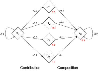Fig. 1 An example of contribution and composition values for an example dataset of five samples. Red values indicate the residual value the model produces for that instance, black values indicate the effects that an instance has upon another. Reproduced from Liu and Barnard under a CC BY 4.0 Deed license.⁵

What this produces is a “CC-matrix” Φ where each row ϕ_i is the Shapley value of the ith instance which consists of n values representing how much the ith instance affects the model predictions of the n other instances in the dataset (including i itself).

The most notable motivation behind the CC values is that influential instances are not equally influential across the spectrum of all the input data. In particular, some types of instances are important when making predictions on other specific (possibly related) examples. This decomposition framework views the data not in terms of points in feature space (instances) but in terms of behaviours; how instances interact with the other instances in the dataset and the model. This means that some materials are more important than others, and will influence other materials differently.

By plotting the contribution and composition values against each other for each instance we obtain a “CC-plot” which is a valuable data visualisation strategy. This visualisation essentially serves as a model- and data-agnostic method of dimensionality reduction into the two CC axes. An example of a CC-plot can be seen in Fig. 2, where positive contribution values indicate that instances work to make the model worse, and negative contributions work to improve the performance of the model. We see in Fig. 2 that the majority of the instances lie around the origin indicating that the impacts of their composition and contribution values are relatively low. Instances with larger feature values (the yellow instances) tend to have significantly larger contributions and make the model worse. This is often the case with data that does not fit the trend of the model or arose from a different distribution (outliers) and warrants further investigation. For this particular data set (the Boston Housing benchmark set), it is known that there was a truncation process applied to houses with a value >50 (thousand). As a result of the truncation process, the houses with larger (yellow) median values are not entirely correct data samples, and it is therefore suggested to remove this data to improve the model fit. To improve the model, more of these types of samples must be gathered or a piece-wise approach should be taken based on the two groups of yellow and non-yellow instances.

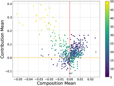Fig. 2 A CC-plot of the well-known Boston Housing dataset²² in machine learning for a linear regression model coloured by the median house value (1000 s). Reproduced from Liu and Barnard under a CC BY 4.0 Deed license.⁵

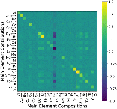
The CC values can also be used to analyse the pairwise effects of instances upon the model predictions upon another in the form of a heatmap. Returning to our focus on materials informatics, a CC heatmap reveals how much each element contributes to the residual errors across the rows and the composition of each of the residuals is given in the columns. Individual cells (scaled to [−1,1]) in the heatmap based on some element represent how much particular types of materials contribute to one another and can uncover hidden interactions from within the data.

It is known that data is more than the sum of its parts, particularly when fitting models for the inference and prediction tasks. The interactions between the instances present in a dataset can increase or decrease the performance of the model which the CC framework seeks to analyse quantitatively. This is just as applicable to data instances as to features, relevant frameworks such as SISSO²³ seek to identify low dimensional descriptors which ‘aggregate’ (by means of dimensionality reduction) the most relevant groups of features together to improve model performance for materials data. Other feature engineering and analysis approaches such as SHAP²¹ and feature selection seek to identify the most relevant features under a certain model. The Shapley Taylor interaction index²⁴ extends the concept of Shapley values to attribute model outputs to the interactions between features. In contrast with features, the concept of interactions is significantly more important when discussing features. Most models are not simply the intersection of a disjoint set of data points, but a mathematical representation of how they interact together, we demonstrate in this work that taking such an interpretation can provide insights into possible actions to take when analysing materials data.

3 Results and discussion

3.1 Dilute solute diffusion dataset

In this section, we present an interpretation of the publicly available solute diffusion dataset²⁵ which includes host and solute pairs and describes the energy of the diffusion energy barriers between these element pairs. This dataset contains more than 230 dilute solute diffusion systems comprising Mg, Al, Cu, Ni, Pd, and Pt host lattices and was previously generated using high-throughput density functional theory (DFT) simulations.

The host–solute diffusion problem has previously been studied using statistical and machine learning techniques for the task of predictive inference.^16,26 This predictive task is useful in determining the energy barriers, and therefore applications of potential new and unknown host–solute pairs, particularly when no experimental data exists. We view this problem through a data and instance analysis lens where we are interested in the effect that the individual host–solute pairs play upon the model. The information gathered can be useful in determining where the deficiencies of existing models may lie, along with what kinds of data may be more valuable or relevant in the future.

Our dataset consists of 408 host–solute pairs, each with 27 features; two of which are the host, and solute elements themselves, along with raw and normalised barrier diffusion energies in eV.²⁷ The normalised barrier diffusion energy is calculated by subtracting a baseline value from the raw diffusion energy based on the main host–solute pair that consists of the same elements (i.e. we subtract the Ag–Ag diffusion energy from all Ag–δ pairs where δ is any element). While this normalisation is well founded in chemistry, physics, and materials science to separate the particularly slow diffusers (i.e. tungsten), the effect this transformation has on the data has never been fully quantified which we attempt to in this section. Using residual decomposition will measure the impact of this ubiquitous correction since what might make sense to domain experts does not necessarily translate well to algorithmic approaches when modelling the data. Additionally, we compare the impacts that this transformation has upon traditional statistical regression models and analyse the impacts that it may have on the assumptions or quality of fit.

3.1.1 Initial regression model. We begin by fitting a simple linear regression to the raw barrier diffusion energies, achieving an adjusted R² score of 0.88. The diagnostic plots determine how well this model fits, as shown in the residual and QQ plots (Fig. 3 and 4). In this case, the residuals show two major groupings of the model mispredictions and a trend potentially containing a dip towards the central values (2 eV to 4 eV) of the data suggesting some presence of non-linearity in the data. We also observe that the tails of the QQ plot deviate from the ideal distribution. Additionally, an inspection of the associated variance inflation factors (VIFs) suggests that some multicollinearity exists among the features.²⁸ The first step to addressing these issues is making use of well-known feature selection strategies including, backwards, forwards, and LASSO selection.¹⁷

Fig. 3 Residual plots for the linear model with all the raw features (top), and fitted using interaction terms of the features (bottom). The red trend line shows the average residual across fitted values.

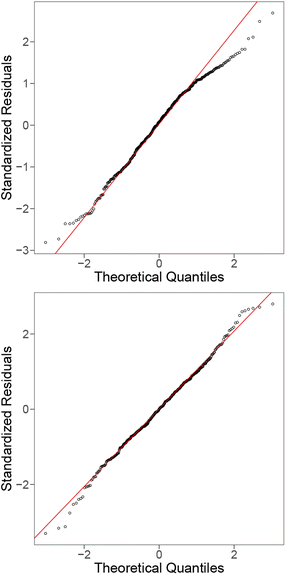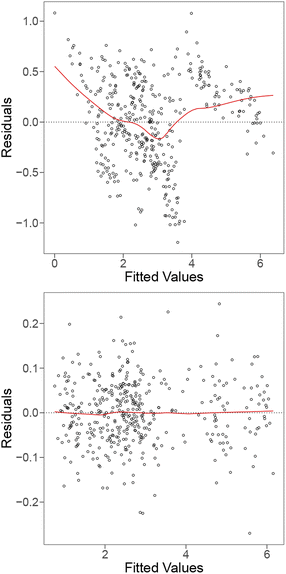
Fig. 4 QQ plots for the linear model with all raw features (top), and fitted using interaction terms of the features (bottom). The red trend line ideal distribution.

By applying feature selection strategies we can reduce the number of features to 17, 15, and 21 physicochemical features respectively with lower VIFs and no loss in the adjusted R² scores. However, the reduction of features does not significantly change the trend in the residual plot and suggests that simple feature selection is not sufficient to optimise the model. The linear model fit may be improved by fitting interaction feature terms.

To further improve our model (to be competitive with ML models), we include interaction terms, where pair-wise interaction between features is considered. The main motivation for this is that some features are related to the host elements, whereas others are related to the solute, and that the relationship between the raw barrier diffusion energies and the host features could be dependent upon the value of the other (solute) features. The final model including interaction terms produces an R² value of 0.995. Fig. 3 and 4 (bottom) show the residual and QQ plots produced for the best model after including interaction terms and applying LASSO as a feature selection strategy. It is much more well-behaved compared to the original model, as indicated by the removal of the U-shaped trend from the residual plot and the approximate normality from the QQ plot.

We now consider an instance-level analysis of this final model based on Cooks' distances. Fig. 5 shows the Cook's distance value for each observation derived from the final model produced. Based on a relative comparison of the Cook's distances, the presence of influential outliers is detected in the data as indicated by the instances with relatively large Cook's distances compared to the others. These outliers are the three pairs: Al–Ce, Ca–Ag, and Ca–Nb, which all contain earth-abundant elements and possess some corrosion resistance and thermal properties that make them suitable for automotive and aerospace applications, and all have been used as catalysts.

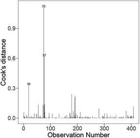Fig. 5 Distribution of the Cooks' distance for each instance on the best model from Fig. 3 (bottom).

Through further examination, we find the magnitude of the standardised residuals for these three instances is large, where Al–Ce, Ca–Ag, and Ca–Nb instances are ranked 8th, 1st, and 6th, respectively, out of the 408 instances. Additionally, these three instances have high leverages, with Al–Ce, Ca–Ag, and Ca–Nb instances being ranked 13th, 4th, and 7th, respectively. The high leverage of Al–Ce is because of its host element (Al) having the smallest host ionic radius and its solute element (Ce) having the largest number of unfilled D-valence electrons in the dataset, while the high leverages of Ca–Ag and Ca–Nb are due to their host element (Ca) possessing the largest host covalent radius, smallest host electronegativity and host Mendeleev number (and the solute element of Ca–Ag having the smallest solute Nd valence unfilled value) among the 408 host–solute pairs. Consequently, these instances are flagged as influential through Cook's distance plot, where their relatively high Cook's distances are mainly contributed by their large standardised residuals and high leverages.

3.1.2 Machine learning analysis. To explore the impact of non-linearity we consider random forests,¹ which are a well-known class of models used in machine learning shown to perform well for materials data,^29–31 along with a linear regression model. The R² values produced by the random forest when fitting to the raw activation barrier energies are close to 1.0 without any significant data processing and contrast with the model steps taken in the previous section. This is an example of where machine learning diverges from statistics, focusing more on how well the model generalises to unseen data (i.e. for the task of predicting properties of unknown host–solute pairs) rather than how well the model fits.

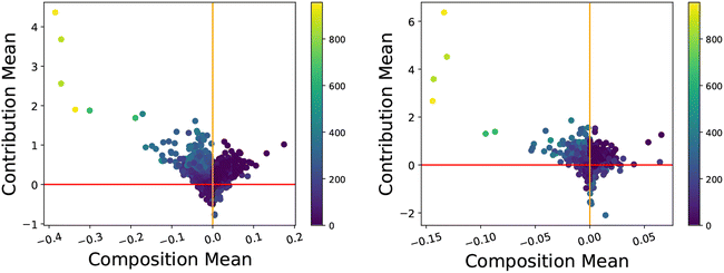
Fig. 6 shows the CC plots for the two models trained on the full set of data to predict the raw diffusion energies. It can be seen that the random forest model (centre) is a significantly better fit for the data than the linear model (left) as the residuals and instances effects are more uniformly distributed and centred at 0. The host–solute pairs with larger diffusion barrier energies (yellow) are poorly behaved, compared to the random forest model where the effects are more symmetric, which confirms that the linear regression model is a poor fit for the data compared to the random forest. Fig. 6 (right) shows the effects on the model when the normalisation scheme is applied. By comparing the centre and right plots we can see that the slow diffusers such as W have less impact on the model, and the contribution values tend to be lower which achieves the stated goals of normalising these types of data. The CC-plot however becomes less symmetric when using the normalised diffusion barrier values compared to the original data and produces a slightly worse fitting model with a lower R² value (0.99 vs. 0.98). Despite this, the 5-fold cross-validation score of the normalised model is significantly higher than that of the raw values. This is precisely because the different behaving instances like W have smaller effects resulting in much lower changes to the model predictions when other more useful samples are removed. As a result, the extrapolation accuracy of using a model with normalised diffusion energies is significantly higher, as evidenced by a cross-validation RMSE score of 0.09 compared to the raw model of 0.12, which is in line with the best performing models developed by Wu et al.¹⁶

Fig. 6 CC-plots for linear regression (left, R² = 0.90) and random forest (centre, R² = 1.00) models trained to predict the raw diffusion energy, and random forest model (right, R² = 0.99) predicting the normalised diffusion energy of the host–solute pairs. Coloured by the diffusion energy level (eV) of the selected samples.

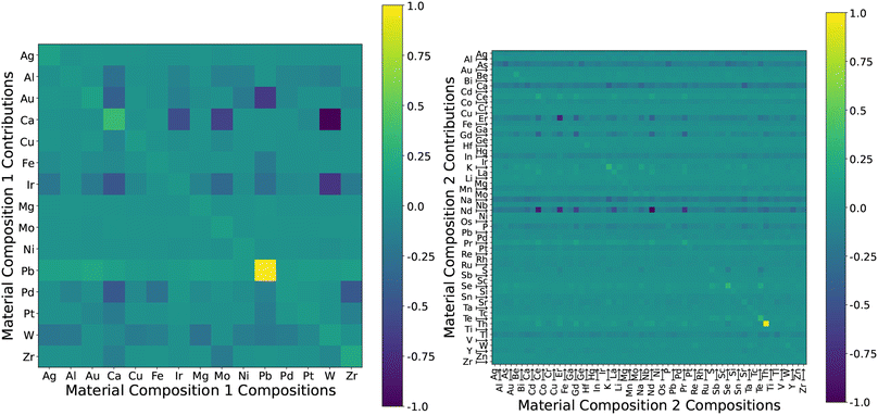
To determine what types of materials have significant impacts on the model, we can break down the CC information into a heatmap, as seen in Fig. 7. The effects that instances have on the model can be unevenly distributed across the dataset. We observe that materials with a Pb host have the greatest effect on other Pb hosts and tend to slightly increase the errors of all other solutes. At the same time, the other host elements (other than Au) have little effect on the predictive outcomes of Pb as seen in the Pb column in Fig. 7 (left). This suggests that there may be some special characteristics or outliers among the properties of Pb hosts. Ca hosts have a different effect compared to Pb hosts, where Ca tends to significantly improve the predictive performance of Ir, Mo, and W hosts. We find these two elements to be the most influential, which is consistent with previous studies that found that the predictive performance of machine learning models for Ca and Pb hosts is inferior compared to the other elements.³² The CC-plot confirms that the effects of these two elements are greatest, but the largest contributor to errors associated with Pb hosts is the Pb data itself, and this is not the case for Ca. We can suggest that, apart from generating more data regarding Ca and Pb hosts, the related elements from the heatmap with impacts on Ca (Pd, Ir, Au, Al) and Pb (Au, Ir) predictions are also of interest. Additionally, despite being particularly slow diffusers, and hence having much higher energy values, the W elements do not significantly increase the loss of the model. The two elements that increase the quality of predictions the most are Ir and W.

Fig. 7 Heatmaps showing how instances with varying host (left) and solute (right) elements contribute to the model. Coloured by the normalised contribution/composition values that each element has upon another's predicted outputs.

We group instance contributions by their solute material composition in Fig. 7 (right) instead of by their host elements (left). There are a significantly larger number of solutes available. The most impactful are the Th–Th, and K–K contributions though again, they do not significantly affect other predictions. The row-wise elements that do decrease the errors (and increase prediction quality) are As, Ca, Er, Gd, Na, and Nd.

The contribution heatmap also informs us of the types of materials that are most useful for the prediction of a particular element. For example, if we are interested in improving the prediction of solutes containing W as a host, we should look into the relevant Ca and Ir elements, along with increasing relevant Pb and W samples since they are most responsible for the prediction errors. If W is the focus, Ca, Ir and Pb could be worth the investment.

3.2 Perovskite forming dataset

In this section, we present a similar interpretation and analysis of the perovskite forming dataset^33,34 which describes the material composition of various perovskite materials. This dataset contains the component elements of the perovskite divided into (up to) the three elements present at the A, B, and X sites. There are 70 features and 1929 sample instances, with two energy levels that may serve as the target prediction labels; the energy above hull (meV) which directly measures the stability based on convex hull analysis,³⁴ and the formation energy (eV) of the system. In this study, we will focus on the energy above hull as it is a more difficult target and is consistent with previous studies.^34,35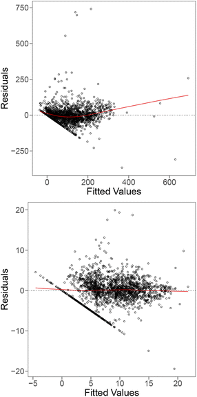

3.2.1 Initial regression model. Beginning with a statistical analysis and considering the regression diagnostics of the model, Fig. 8 (top) shows a relatively poor simple linear model fitting the data to the level of the energy above hull (meV) with an adjusted R² score of 0.64. The residual plot displays a slight U-trend and a notably larger spread of residual values in the range of 100–200 meV fitted values, with the latter suggesting the issue of heteroskedasticity. There are also highly non-ideal values in the upper and lower ends of the QQ plot (Fig. 9). Again, backwards, forwards, and LASSO selection strategies are used to reduce the severe multicollinearity issues given the large number of features.

Fig. 8 Residual plots for the linear model with all the raw features (top), and fitted using interaction terms of the features (bottom) for the perovskites dataset.

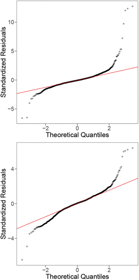Fig. 9 QQ plots for the linear model with all raw features (top), and fitted using quadratic terms of the features (bottom) for the perovskites dataset.

To deal with the issues in the residuals, we considered a square-root transformation for the energy above the hull and incorporated pair-wise interaction terms of the features into the model as some features are associated with the elements in A site while the others are related to the elements in B site. When adding interaction terms to the model, some features had to be excluded due to their high degree of discreteness, it appears that many of the tested linear models struggled with this data due to the number of discrete features in the data. We observe that the square-root transformation of the energy above the hull and inclusion of additional pair-wise interaction terms produce a significantly flatter trend and more consistent spread (homoskedasticity) for the residual plot in Fig. 8 (bottom). A line is also formed from the residuals of instances with 0 meV energy above hull in the residual plot. However, it can be observed that the QQ plot (Fig. 9 (bottom)) still demonstrates deviations from the ideal line. This suggests that a linear model may not be the best fit for this dataset either.

Across the tested linear models, the set of influential materials identified by Cook's distance in Fig. 10 is largely similar. The materials we found to be influential across models were Ba₈Mo₈O₂₄, Mg₈Fe₈O₂₄, Y₄Ba₄Mn₂Fe₆O₂₄ and Y₄Sr₄MnNi₇O₂₄. Additional investigation into these influential materials found that they all have large magnitudes of standardised residuals around the value of 5 (except for Mg₈Fe₈O₂₄ with 2.7), and relatively higher leverages compared to the rest of the materials (except for Ba₈Mo₈O₂₄), where the latter is primarily due to some of their features taking extremely large/small values. For instance, Mg₈Fe₈O₂₄ has the largest difference in the specific heat capacity between A and B sites, Y₄Ba₄Mn₂Fe₆O₂₄ has the largest first ionisation potential averaged across A and B sites. In contrast, Y₄Sr₄MnNi₇O₂₄ has a large ionisation energy averaged across A and B sites. Finally, the energy above hull of Ba₈Mo₈O₂₄, Mg₈Fe₈O₂₄ and Y₄Ba₄Mn₂Fe₆O₂₄ are 643.73 meV, 636.34 meV, and 950.23 meV, respectively, which are much larger than the energy above hull of the other material instances that are mostly concentrated in the range of 0–400 meV. In summary, the combination of large standardised residuals, high leverages, and extreme energy above hull resulted in these materials being identified as influential instances in the fitted models.

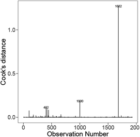Fig. 10 Distribution of the Cooks' distance for each instance on the best model from Fig. 8 (bottom).

3.2.2 Machine learning analysis. We continue with the analysis of a linear model and random forest using CC plots. Once again the random forest produces a higher R² = 0.95 value compared to the linear model with a value R² = 0.58, as shown in Fig. 11. The fit is noisy with a large number of samples lying far from the central mass, which suggests that many of the perovskites are unique or the model fails to learn the behaviours well.

Fig. 11 CC-plots for the linear model (left, R² = 0.58) and random forest (right, R² = 0.98) for perovskite dataset predicting the energy above hull (meV). Coloured by the energy above hull (meV) value for each instance.

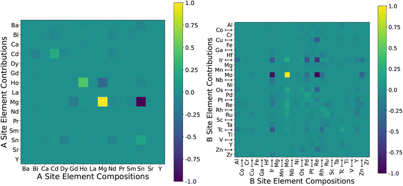
The contribution interactions between the material contributions are shown in the heatmaps for the A and B site main elements in Fig. 12. We note that this form of data visualisation may not be fully representative of this dataset since there are up to three elements at the A and B sites but we can only capture and visualise the main (first) one since there are sometimes no elements at the second and third sites. Other than the self-element interactions (i.e. Mg to Mg), there are relatively few highly interacting groups of A site elements, and the two main ones are Ho–Mg, and Mg–Sn. An observation we can make here is that there is a significant difference when having elements as the first or second A site element. For example, there is only a single perovskite with Mg as the first element at the A site, but many more as the second element at the A site, and there is a significant difference in their energy above hull levels and may be contributing to the poorer model fit. This again could be attributed to the low sample size where there is only one instance of each Mg, and Sn, or the poor visual representation given that there are a significant number of samples with these elements as the second or third element at the A site. When we consider the B site in Fig. 12 (right), we see several elements with effects that stand out from the rest, notably Ir and Mo for contributions effects and Ir, Mo, Pd, and Re for the composition effects. Again, there is a significant data imbalance within this attribute, and these elements only contain a single sample and produce large impacts on the model.

Fig. 12 Heatmap showing the contribution effects of effects that each instance has upon each other based on Shapley residual decomposition. Pairwise contribution based on A site #1 (left) and B site #1 (right). Coloured by the normalised contribution/composition that each element has upon another's predicted outputs.

These materials could be removed, or more resources dedicated to gathering more data. Due to the extreme effects that these perovskites have upon the model, and the differences between their energy levels and the rest of the data, we suggest the removal of these materials. The net effect that they have upon the model is negative and does not aid in predicting similar materials as evidenced by their large residual errors when predicting themselves. It is unlikely more data would give a return on the investment.

3.3 Metallic glass dataset

The metallic glass dataset contains 585 material samples and 20 features consisting of descriptors of the composition of the material, and two additional features detailing the chemical formula along with the main element involved. The glass transition temperature (trg) is an approximate indicator for the glass forming ability (GFA) of each alloy which can be used as a target label for predictive tasks.^36,37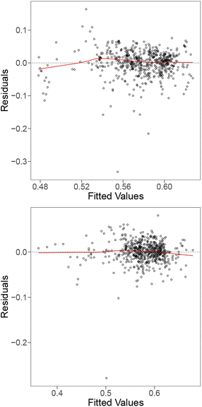

3.3.1 Initial regression model. When fitting the linear model to the data we observed serious multicollinearity issues in this dataset, in particular, between specific heat capacity and heat capacity mass. As a result, we begin with the feature selection using LASSO to drop some of these highly correlated features, then fit a model that includes pair-wise interaction terms of the selected features. For brevity, we directly consider the best model produced which made use of the interaction terms here. The residual and QQ plots are shown in Fig. 13 and 14, where we observe that the distribution of residuals is relatively flat across the fitted values, but there are significant deviations from the tails of the QQ plots.

Fig. 13 Residual plots for the linear model with all the raw features (top), and fitted using interaction terms of the features (bottom) for the metallic glass data.

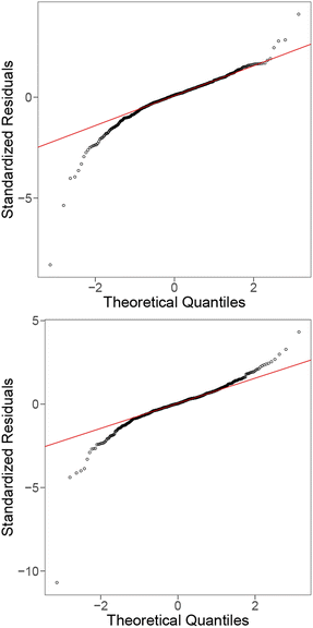Fig. 14 QQ plots for the linear model with all raw features (top), and fitted using interaction terms of the features (bottom) for the metallic glass data.

To interpret the outliers based on the model containing feature interaction terms from Fig. 15, namely Au₃₅Ca₆₅, Ga₈Sr₈₂ and Pt₄₂·5Cu₂₇Ni₅₉·5P₂₁. These instances all have leverages ∼0.99, primarily due to some of their features taking extremely large/small values. For example, Au₃₅Ca₆₅ has the smallest B composition average and site1 heat capacity mass, Ga₈Sr₈₂ has the smallest IsDBlock composition average, and Pt₄₂·5Cu₂₇Ni₅₉·5P₂₁ has the largest site1 density. Their extremely high leverages combined with their relatively large standardised residuals (1.44, 1.79, and −3.86 for Au₃₅Ca₆₅, Ga₈Sr₈₂, and Pt₄₂·5Cu₂₇Ni₅₉·5P₂₁, respectively) resulted in them being influential materials. Overall the presence of these outlying terms had a significant impact on the regression model and poses a challenge to model fitting.

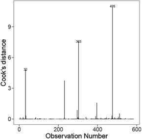Fig. 15 Distribution of the Cooks' distance for each instance on the best model from Fig. 13 (bottom).

3.3.2 Machine learning analysis. Fig. 16 shows the CC plots for the linear and random forest models to predict the glass transition temperature. We observe the characteristic V-shaped plot which is commonly seen among poor-performing models where few points reduce the magnitude of the errors in the model,⁵ This V-shaped curve is a result of a large number of instances with large residual values (large composition mean) which results in a larger number of instances producing large contribution values which correspond to those large residuals. The linear model is a poor fit to the data with a low R² = 0.27 score along with the V-shaped nature of the CC plot. The random forest model performs significantly better and has a much larger number of subzero contribution values which increases the quality of the predictions, despite the difference in model performance, the most impactful materials remain consistent across both models. However, there remains asymmetry in the contribution effects signifying possible problems with the data itself. One notable aspect of this data is the imbalance in the trg values where there are fewer materials with trg values <0.4, with a single small outlier with trg = 0.2. Furthermore, we observe a large number of deviations from the central group which may indicate poor coverage of the data space or the presence of outliers. This indicates that this dataset contains significant selection bias that is common among materials datasets that were not originally generated with machine learning in mind.¹³

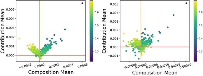Fig. 16 CC-plots for the linear model (left, R² = 0.27) and random forest (right, R² = 0.92) for the metallic glass dataset coloured by the glass transition temperature.

Within this dataset, there are many main element groups with only a small number of materials, sometimes even only one instance (such as Ho), and the effects of this sampling procedure are reflected in the heatmap shown in Fig. 17. We observe that there is a ‘spotted’ quality, where many of those same materials with a low number of samples contribute to producing larger error values. Similar to the linear model previously considered in Section 3.3.1, the impact of these outliers in the model and data is significant, even though the outliers we observe for the random forest are different compared to the linear model. Glasses with Er and Sc main elements were the most responsible for making the model worse and interacted with other model predictions, whereas Pt had a similar effect on itself but seemed to fit the general trend and had little negative impact upon other main element predictions. A greater variety of Pt-rich glasses could be added without compromising model performance or affecting other instances, suggesting this is a safe and effective way of progressing this research.

Fig. 17 Heatmap showing the contribution effects of effects that each instance has upon each other based on Shapley residual decomposition. Pairwise contribution based on the main element present in the metallic glass. Coloured by the normalised contribution/composition that each element has upon another's predicted outputs.

4 Conclusion

In this paper, we presented an analysis of three established datasets in the materials sciences, exploring the impact of domain-driven normalisation, extreme values, and selection bias. Our analysis includes fitting a linear model and using influence statistics to analyse the effects that particular influential samples may have had on the model. We extend this analysis using the residual decomposition framework to analyse and compare the instance insights derived from statistical and machine learning methods. These insights can provide a deeper analysis of the materials data, or inform future data-gathering processes to gather sample that fits better models.

In general, across the three datasets, we identified several materials that were problematic and significantly impacting the model fit. From a statistical perspective, these materials manifested as outlying extreme values in the model diagnostic plots. From a machine learning perspective, they had high contribution and composition values resulting in significant changes in model performance. The residual decomposition framework can inform us of the appropriate treatment of these types of materials, including removal as outliers, gathering more specific data, or rebalancing the dataset using oversampling or imputation.

Our workflow approach is entirely general, and can also be used as forensics to quantify the impact of practical decisions that are made by researchers during data acquisition, cleaning, and processing. We have provided an example in Section 3.1 where the impact of applying data normalisation can be compared with the model trained on the raw energy values. Not all materials are equally important in materials informatics, and predictions can be improved by focusing more attention on the materials that are. At the same time, quantifying the types of data which even slightly deviate from each other can provide greater insights into why or how the phenomena are generated from the representative inputs if the inference task is the goal. If the predictive ability is the only criterion, removing the outlying instances tends to significantly improve model performance.

Data availability

The code, analysis scripts, and datasets supporting this article have been uploaded as part of the ESI.† All data is publicly available from the referenced links: processed and final datasets are compiled by Morgan.^27,35,37 and are publicly available at https://figshare.com/articles/dataset/MAST-ML_Education_Datasets/7017254. The software is available at: https://doi.org/10.6084/m9.figshare.24797277.v3.

Author contributions

Tommy Liu: conceptualisation, methodology, writing – original draft, investigation, software, formal analysis, validation, visualisation. Zhi Yang Tho: methodology, formal analysis, visualisation, writing – original draft. Amanda. S. Barnard: conceptualisation, writing – review & editing, supervision, project administration, data curation, resources.

Conflicts of interest

There are no conflicts to declare.

Acknowledgements

This research was supported by the National Computational Infrastructure (NCI) under project p00, and the Australian Government under an Australian Government Research Training Program (RTP) Scholarship.

Notes and references

1. L. Breiman, Stat. Sci., 2001, 16, 199–231.
2. C. M. Bishop, Pattern Recognition and Machine Learning (Information Science and Statistics), Springer-Verlag, Berlin, Heidelberg, 2006.
3. C. Molnar, Interpretable Machine Learning, 2nd edn, 2022.
4. A. Barnard, B. Motevalli, A. Parker, J. Fischer, C. Feigl and G. Opletal, Nanoscale, 2019, 11, 19190–19201.
5. T. Liu and A. S. Barnard, International Conference on Machine Learning, ICML 2023, 23-29 July 2023, Honolulu, Hawaii, USA, 2023, pp. 21375–21387.
6. A. Ghorbani and J. Y. Zou, Proceedings of the 36th International Conference on Machine Learning, ICML 2019, 9-15 June 2019, Long Beach, California, USA, 2019, pp. 2242–2251.
7. G. Pruthi, F. Liu, S. Kale and M. Sundararajan, Advances in Neural Information Processing Systems 33: Annual Conference on Neural Information Processing Systems 2020, NeurIPS 2020, December 6-12, 2020, virtual, 2020.
8. C. Yeh, J. S. Kim, I. E. Yen and P. Ravikumar, Advances in Neural Information Processing Systems 31: Annual Conference on Neural Information Processing Systems 2018, NeurIPS 2018, December 3-8, 2018, Montréal, Canada, 2018, pp. 9311–9321.
9. R. D. Cook, J. Am. Stat. Assoc., 1979, 74, 169–174.
10. S. Chatterjee and A. S. Hadi, Stat. Sci., 1986, 1, 379–393.
11. M. B. Tofanelli and S. E. Wortman, Agronomy, 2020, 10, 1618.
12. A. Azari, R. Nabizadeh, S. Nasseri, A. H. Mahvi and A. R. Mesdaghinia, Chemosphere, 2020, 250, 126238.
13. A. S. Barnard, B. Motevalli, A. J. Parker, J. M. Fischer, C. A. Feigl and G. Opletal, Nanoscale, 2019, 11, 19190–19201.
14. J. B. Gray, Technometrics, 2002, 44, 191–192.
15. A. Schneider, G. Hommel and M. Blettner, Deutsches Ärzteblatt International, 2010, 107, 776.
16. H. Wu, A. Lorenson, B. Anderson, L. Witteman, H. Wu, B. Meredig and D. Morgan, Comput. Mater. Sci., 2017, 134, 160–165.
17. R. Tibshirani, J. Roy. Stat. Soc. B, 1996, 58, 267–288.
18. P. W. Koh and P. Liang, Proceedings of the 34th International Conference on Machine Learning, ICML 2017, Sydney, NSW, Australia, 6-11 August 2017, 2017, pp. 1885–1894.
19. R. Kohavi, Proceedings of the 14th International Joint Conference on Artificial Intelligence – Volume 2, San Francisco, CA, USA, 1995, pp. 1137–1143.
20. S. Tang, A. Ghorbani, R. Yamashita, S. Rehman, J. A. Dunnmon, J. Zou and D. L. Rubin, Sci. Rep., 2021, 11, 8366.
21. S. M. Lundberg and S. Lee, Advances in Neural Information Processing Systems 30: Annual Conference on Neural Information Processing Systems 2017, December 4-9, 2017, Long Beach, CA, USA, 2017, pp. 4765–4774.
22. D. Harrison and D. L. Rubinfeld, J. Environ. Econ. Manag., 1978, 5, 81–102.
23. R. Ouyang, S. Curtarolo, E. Ahmetcik, M. Scheffler and L. M. Ghiringhelli, Phys. Rev. Mater., 2018, 2, 083802.
24. M. Sundararajan, K. Dhamdhere and A. Agarwal, International conference on machine learning, 2020, pp. 9259–9268.
25. H. Wu, T. Mayeshiba and D. Morgan, Sci. Data, 2016, 3, 1–11.
26. C. D. Versteylen, N. H. van Dijk and M. H. F. Sluiter, Phys. Rev. B, 2017, 96, 094105.
27. D. Morgan, T. Mayeshiba and D. Morgan, DFT dilute solute diffusion in Al, Cu, Ni, Pd, Pt, Mg, Fe, W, Mo, Au, Ca, Ir, Pb, Ag, Zr, 2018, https://figshare.com/articles/dataset/DFT_dilute_solute_diffusion_in_AlCu_Ni_Pd_Pt_and_Mg/1546772.
28. J. Neter, W. Wasserman and M. Kutner, Applied Linear Regression Models, Irwin, 1989.
29. A. Agrawal and A. Choudhary, APL Mater., 2016, 4, 053208.
30. J. Wei, X. Chu, X.-Y. Sun, K. Xu, H.-X. Deng, J. Chen, Z. Wei and M. Lei, InfoMat, 2019, 1, 338–358.
31. K. Song, F. Yan, T. Ding, L. Gao and S. Lu, Comput. Mater. Sci., 2020, 174, 109472.
32. K.-n. He, X.-s. Kong and C. Liu, Comput. Mater. Sci., 2020, 184, 109948.
33. R. Jacobs, T. Mayeshiba, J. Booske and D. Morgan, Adv. Energy Mater., 2018, 8, 1702708.
34. W. Li, R. Jacobs and D. Morgan, Comput. Mater. Sci., 2018, 150, 454–463.
35. T. Mayeshiba and D. Morgan, Dataset for Factors controlling oxygen migration barriers in perovskites, 2018, https://figshare.com/articles/dataset/Dataset_for_Factors_controlling_oxygen_migration_barriers_in_perovskites/7180817.
36. Z. Lu, Y. Li and S. Ng, J. Non-Cryst. Solids, 2000, 270, 103–114.
37. B. Afflerbach, L. Schultz, J. H. Perepezko, P. Voyles, I. Szlufarska and D. Morgan, Data for “Molecular Simulation-derived features for machine learning predictions of metal glass forming ability”, 2021, https://figshare.com/articles/dataset/Data_for_Molecular_Simulation-derived_features_for_machine_learning_predictions_of_metal_glass_forming_ability_/13202912.

---

Footnote

† Electronic supplementary information (ESI) available. See DOI: https://doi.org/10.1039/d3dd00171g

---