 Open Access Article
Creative Commons Attribution 3.0 Unported Licence
Semi-supervised learning of images with strong rotational disorder: assembling nanoparticle libraries†
Maxim A.
Ziatdinov
*a,
Muammer Yusuf
Yaman
 b,
Yongtao
Liu
c,
David
Ginger
b and
Sergei V.
Kalinin
ad
aPhysical Sciences Division, Pacific Northwest National Laboratory, Richland, WA 99354, USA. E-mail: maxim.ziatdinov@pnnl.gov
bDepartment of Chemistry, University of Washington, Seattle, WA 98195, USA
cCenter for Nanophase Materials Sciences, Oak Ridge National Laboratory, Oak Ridge, TN 37831, USA
dDepartment of Materials Science and Engineering, University of Tennessee, Knoxville, TN 37996, USA
First published on 21st May 2024
Abstract
The proliferation of optical, electron, and scanning probe microscopies gives rise to large volumes of imaging data of objects as diversified as cells, bacteria, and pollen, to nanoparticles and atoms and molecules. In most cases, the experimental data streams contain images having arbitrary rotations and translations within the image. At the same time, for many cases, small amounts of labeled data are available in the form of prior published results, image collections, and catalogs, or even theoretical models. Here we develop an approach that allows generalizing from a small subset of labeled data with a weak orientational disorder to a large unlabeled dataset with a much stronger orientational (and positional) disorder, i.e., it performs a classification of image data given a small number of examples even in the presence of a distribution shift between the labeled and unlabeled parts. This approach is based on the semi-supervised rotationally invariant variational autoencoder (ss-rVAE) model consisting of the encoder–decoder “block” that learns a rotationally-invariant latent representation of data and a classifier for categorizing data into different discrete classes. The classifier part of the trained ss-rVAE inherits the rotational (and translational) invariances and can be deployed independently of the other parts of the model. The performance of the ss-rVAE is illustrated using the synthetic data sets with known factors of variation. We further demonstrate its application for experimental data sets of nanoparticles, creating nanoparticle libraries and disentangling the representations defining the physical factors of variation in the data.
Introduction
The proliferation of optical, electron, and scanning probe microscopies continues to give rise to large volumes of imaging data.1–4 For biological systems, this includes objects as diversified as cells, bacteria, organelles, and pollen.5–7 In nanoscience this includes nanoparticles, nanowires, and other nano-objects.8–10 In electron and scanning probe microscopy, this includes atoms and molecules as detected via changes in the local density of states or nuclei density.11–14.11–14 Correspondingly, there is considerable interest in deriving physical information and potentially actionable insights from these images, ranging from the identification and classification of the defects,15–17 reconstruction of the statistical and generative18,19 physical models, or identification of medical conditions and potential interventions.20In many cases, the data streams coming from the imaging systems contain the objects with a strong translational and rotational disorders, since the objects of interest typically have arbitrary orientation and position in the field of view.21,22 For example, in crystalline materials, the preferred orientation is determined by the relevant alignment of the crystallographic axes with respect to the image plane, with potentially small disorder due to local and global strains and scan distortions. At the same time, for mesoscale imaging and disordered materials, the objects of interest can have arbitrary orientation in the image plane. Analysis of these data streams necessitates rapid classification and identification of the observed objects. An often-encountered scenario is the one in which the individual objects are separable, corresponding to the strong dilution of original solution,23–26 rare defects,27–30 or easily identifiable borders of the objects.31–35 In these cases, the compound images containing multiple objects can be separated into the patches containing individual objects of interest, albeit at arbitrary orientation, with positional jitter relative to the center of the patch due to the variability of object shapes. Correspondingly, analysis of such data via supervised or unsupervised machine learning methods needs to account for these factors of variability.
Supervised learning, known for its ability to learn complex patterns and achieve precise prediction using labeled data, is very suitable for tasks such as classification and regression.36 However, supervised learning requires a large amount of labelled data (time-consuming), and it can also struggle with generalization with the input data and the training data are significantly different. In contrast, unsupervised learning is particularly valuable in terms of unstructured and unlabeled data by enabling data understanding, which is also inherent with the limitations in its ambiguity of understanding specific patterns that are irrelevant to the tasks. Therefore, semi-supervised learning, in which a small number of labels is provided, combines the merits of both supervised and unsupervised learning, become necessary.37 The approach of semi-supervised learning corresponds to the practically encountered scenarios where prior data in the form of small manually labeled sets, published papers, catalogs, or other forms is available. There have already been lots of success in literature that apply semi-supervised learning to different datasets varying from dendritic microstructures,23 pathology images, and soft materials.24 The central challenge of such analysis is the generalization from a small subset of labeled data with a weak orientational disorder (e.g., manually labeled data or reference data) to a large unlabeled data set with a much stronger orientational disorder. In the language of deep/machine learning (DL/ML), our goal is to generalize to a dataset characterized by distributional shift, which is one of the key challenges for practical applications of DL/ML models.38
Results
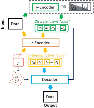
To address this challenge, here we develop an approach for semi-supervised learning based on variational autoencoders with rotational (and translational) invariance. Variational autoencoders (VAE) belong to a class of probabilistic graphical models that can learn the main continuous factors of variation from high-dimensional datasets.39,40 It consists of generative and inference models of the forms p(x|z)p(z) and q(z|x) usually referred to as decoder and encoder. The former treats the latent variable z as a code from which it tries to reconstruct the observation x using a prescribed prior distribution p(z) (here chosen as standard Gaussian), whereas the latter is used to approximate the usually intractable posterior distribution. Both encoder and decoder are parametrized by deep neural networks. The low-dimensional latent representations learned by VAE can be efficiently used for downstream tasks such as classification even with a limited number of labels. More specifically, to use VAE in a semi-supervised learning setting, one treats a class label as one of the latent factors of variation. This latent variable comes from a discrete distribution and is known a priori only for a small fraction of the data. The encoding into the discrete classes for the unlabeled part of data is performed by a separate neural network (y-encoder in Fig. 1), which also plays a role of a classifier. The semi-supervised VAE (ss-VAE) has been successfully applied to standard benchmark datasets such as MNIST41 where it was able to achieve ∼90% accuracy on the dataset with only ∼3% of labels available.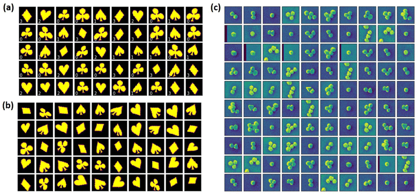 | ||
| Fig. 2 Illustration of the datasets used in this study. (a and b) The representation of the cards dataset as introduced in ref. 28. (a) Typical objects from the labeled part of the dataset with a weak orientational disorder (the rotational angle is sampled uniformly from the [−4°, 4°] range). (b) Typical objects from the unlabeled part of the dataset with a strong orientational disorder (the rotational angle is sampled uniformly from the [−60°, 60°] range). (c) Experimental dataset of the gold nanoparticles. | ||
Unfortunately, the classical ss-VAE struggles to perform accurate classification of the unlabeled data obtained under conditions different from those of labeled data. For example, as we show below, even a relatively small increase in the orientational disorder for the unlabeled portion of data almost completely throws off the classifier. Simply increasing the fraction of labeled data does not lead to improved results since the “new” labeled data still comes from the same distribution.
To overcome this limitation, we partition a continuous latent space of the ss-VAE into the part associated with orientational and positional disorders and the part corresponding to the remaining factors of variation (shear, scale, etc.). The latent variables from the former are used to rotate (and translate) the pixel grid associated with input images, which is then concatenated with the rest (continuous and discrete) latent variables and passed to the VAE's decoder to enforce a geometric consistency42 between rotated (and translated) unlabeled objects. As far as the choice of the decoder's prior for the angle latent variable is concerned, we tested both standard normal distribution and intuitively more suitable projected normal distribution43 (continuous distribution on the circle) and found no significant difference for the datasets used in this paper. The weights of the encoders and decoder are trained by optimizing the standard ss-VAE loss objective with an explicit classification loss for the labeled data.44
As a model synthetic data set, we have chosen the dataset with playing card suites as originally introduced in ref. 45. This choice is predicated on a relatively small number of classes (4), and interesting full and partial degeneracies with respect to the affine transforms. For example, upon compression and 90 degrees rotation the diamond will transform into a (smaller) diamond of the same orientation. For clubs, the rotation by 120 yields an almost identical object shape, allowing to trace the tendency of a model to get captured in metastable minima. Finally, spades and (rotated) hearts differ by the presence of a small tail only.
We generated a data set of M = 12![[thin space (1/6-em)]](https://www.rsc.org/images/entities/char_2009.gif) 000 cards (3000 per each card suite) having the varying angular, translation, shear, and size disorders. In addition, we generated a small number, N = 800 (200 per each card suite), of the labeled examples. Importantly, the labeled examples do not have a positional disorder (the objects are fixed at the center of image) and are characterized by only a negligible orientational disorder part (the objects are rotated in the range between −4° and 4°) compared to the unlabeled part (see Fig. 1a and b). The ss-rVAE training aims to simultaneously address three targets: (i) to reconstruct the data set, (ii) to establish the structure in the latent space, and (iii) to assign the labels to the individual elements of the data set characterized by a distributional shift. Finally, the evaluation of the trained model accuracy was performed on a separate dataset generated using the same disorder parameters as the unlabeled part of the training data but with a different pseudo-random seed. The exploration of ss-VAE with desired invariances can be performed in the provided Jupyter Notebook. The better performance of ss-VAE with rotational invariance can also be observed in ESI Videos S1 and S2,† which show the training processes of ss-VAE without and with rotational invariance, respectively. The corresponding latent space distributions are also shown in Fig. 1, along with the confusion matrices in Fig. S2,† which also indicate the better performance of ss-VAE with rotational invariance. We note that the performance of ss-VAE with rotational invariance can be improved by increasing the ratio of supervised data, as seen in ESI Video S3.†
000 cards (3000 per each card suite) having the varying angular, translation, shear, and size disorders. In addition, we generated a small number, N = 800 (200 per each card suite), of the labeled examples. Importantly, the labeled examples do not have a positional disorder (the objects are fixed at the center of image) and are characterized by only a negligible orientational disorder part (the objects are rotated in the range between −4° and 4°) compared to the unlabeled part (see Fig. 1a and b). The ss-rVAE training aims to simultaneously address three targets: (i) to reconstruct the data set, (ii) to establish the structure in the latent space, and (iii) to assign the labels to the individual elements of the data set characterized by a distributional shift. Finally, the evaluation of the trained model accuracy was performed on a separate dataset generated using the same disorder parameters as the unlabeled part of the training data but with a different pseudo-random seed. The exploration of ss-VAE with desired invariances can be performed in the provided Jupyter Notebook. The better performance of ss-VAE with rotational invariance can also be observed in ESI Videos S1 and S2,† which show the training processes of ss-VAE without and with rotational invariance, respectively. The corresponding latent space distributions are also shown in Fig. 1, along with the confusion matrices in Fig. S2,† which also indicate the better performance of ss-VAE with rotational invariance. We note that the performance of ss-VAE with rotational invariance can be improved by increasing the ratio of supervised data, as seen in ESI Video S3.†
The classification accuracies of the trained ss-VAE (without rotational invariance) and ss-rVAE (with rotational invariance) are shown in Fig. 3a for different orientational disorders in the unlabeled dataset. Here, the labels on horizontal axis show a range from which the angles for the unlabeled data were uniformly sampled. For the sake of brevity, we will refer to each distribution by the value of α that forms the [−α, α] interval. The angles for the labeled data were sampled from a uniform distribution with α = 4° for all the cases. The classification is performed with a y-encoder (see Fig. 1). Clearly, the ss-VAE fails to generalize to the unlabeled data with different orientations of the same objects, with most of the prediction accuracies just slightly above a random guess. Nor it could learn any meaningful latent representation of the data (Fig. 3b). On the other hand, the ss-rVAE applied to the exact same datasets shows a robust classification performance (>75% accuracy) for a relatively broad range of the orientational disorder (4° < α < 90°). Furthermore, the ss-rVAE is capable of learning the correct factors of variation for this range of angular disorder (Fig. 3c). Indeed, the first continuous latent variable (z1) clearly captures a variation in scale whereas the second one (z2) encoded a variation in shear deformation. We note that the accompanying Jupyter Notebook allows readers to explore different ranges of the disorder parameters as well as to tune the architectures (e.g., change a number of layers in the encoder and decoder modules) of the VAE models.
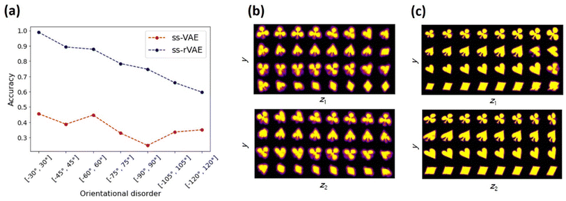 | ||
| Fig. 3 Performance of the ss-VAE (without rotational invariance) and ss-rVAE (with rotational invariance) on the cards dataset. (a) Comparison of the classification performance between the regular (ss-VAE) and rotationally invariant (ss-rVAE) models on the unlabeled test datasets characterized by a distributional shift in the form of increasing orientational disorder. The horizontal axis labels show an interval from which the rotation angles for the unlabeled data were sampled uniformly. The labeled part used in training remained the same in all the cases and corresponded to the data described in Fig. 2a. (b and c) Class-conditioned latent space traversals of the ss-VAE (b) and ss-rVAE (c) learned from the unlabeled data with rotation angles sampled from [−60°, 60°] interval. Note that the first continuous latent variable (top row in (c)) captures variation in scale whereas the second continuous latent variable (bottom row in (c)) corresponds to a shear strain. | ||
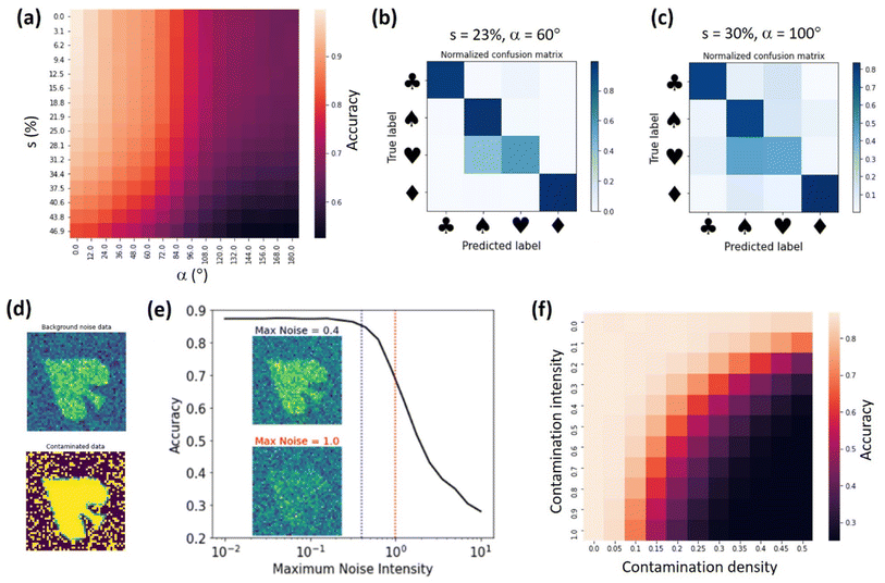
Next, we investigated the performance of the trained ss-rVAE model on datasets with varying disorder and noise levels. We note that such “stress tests” are critical for deploying the ML models online (i.e., during the actual experiments) where one may not have time to retrain a model every time there are changes in the data generation process. Fig. 3b shows a dependence of ss-rVAE prediction accuracy on angular and shear disorder. Here, we use s to denote the [0, s] range from which values of shear deformation are uniformly sampled. The ss-rVAE was trained on the dataset with s = 23% and α = 60°. One can see that ss-rVAE shows a remarkable robustness even when the shear deformation strength exceeds the maximum shear level used in the training dataset. For the orientational disorder, the accuracy is expectedly decreasing for α > 60°, consistent with observations in Fig. 3. Nevertheless, it remains at acceptable levels (>70%) even at the very high rotation angles (up to α = 180°) for the low and moderate shear values. This is remarkable because even though we didn't explicitly enforce the rotational invariance on our classifier (y-encoder), it was learned by the “proximity” to the rVAE part (z-encoder and decoder) of the model. Finally, for the large shear (>30%) and strong orientational disorder (α > 100°) the model struggles to provide accurate predictions. The confusion matrix analysis of the test datasets (Fig. 4b and c) revealed that the misclassification originates mostly from mislabeling hearts to spades, whereas the assignments of all other cards (club, spade, and diamond) remain robust.
To explore noise effects, we introduced two kinds of noise to simulate practical experimental results as demonstrated in Fig. 4d. The first one is a simple Gaussian noise. This type of noise is common in experimental measurements and is sometimes referred to as background noise. Fig. 4e shows the dependence of the ss-rVAE prediction accuracy on the intensity of the background noise dataset. We can see that ss-rVAE predictions are robust to noise with intensities below 0.4. Moreover, even if the noise intensity reaches 1.0, the ss-rVAE still has an accuracy above 70% (the insets in 4e show examples of how the data looks like for noise intensities of 0.4 and 1.0). Noteworthily, we believe that most practical experimental data can maintain a noise intensity below 1.0 or even below 0.4, suggesting that ss-rVAE can have a robust performance in practical use. In addition, we note that this ss-rVAE model is trained on a clean dataset, and therefore its performance on noisy data can be further improved if the model is trained with using data augmented by noise.
For the second type of noisy data, we added an extra signal intensity to random pixels of the clean data. This type of noise is analogous to measuring experimental samples with contamination, so we refer to this data as contaminated data. We defined two parameters to control the contamination level: one is contamination density that is determined by the ratio of pixels with contamination signal; the other is contamination intensity that is determined by the intensity of the added signal. Shown in Fig. 4f is the dependence of ss-rVAE analysis accuracy on contamination level and density. We can see that the ss-rVAE shows good accuracy when the contamination density is below 10%.
We further extended this approach to experimental data, namely the analysis of the gold nanoparticle (GNPs) assemblies. The GNPs were salted with NaCl solution to an indium-tin oxide (ITO) substrate. The process of salting was observed using dark field microscopy to make sure enough GNPs are on the ITO substrate. Then, we performed imaging on the same area using scanning electron microscopy. The nanoparticle dataset is automatically created from the electron micrographs and then hand-labeled manually by us using the number particles in each image as “class”.
Here, we limited ourselves only to classes that have no less than 30 “samples” (images). This left us with four classes corresponding to 1-, 2-, 3- and 4-particle agglomerations, with 304, 93, 49, and 31 images in each class. We took 15 samples from each class to prepare the labeled dataset, whereas the remaining ones went into the unlabeled dataset. Note that this created a significant class imbalance against which we are going to test our ss-rVAE model.
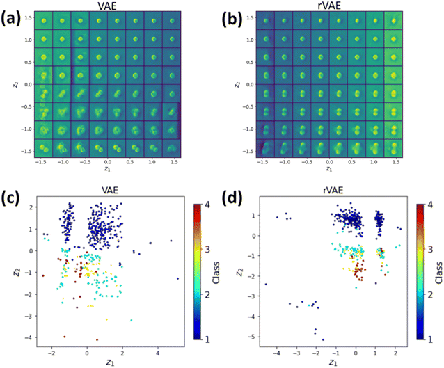
As initial test, we attempted the simple VAE and rVAE approaches (i.e., z-encoder and decoder only, without (VAE) and with (rVAE) partitioning of the continuous latent z-space). Fig. 5 shows the latent space and distribution of the encoded latent variables of VAE and rVAE analyses. In this case, the training is completely unsupervised and no classification is performed (albeit the distribution of the data in the latent space can provide indication on feasibility of the latter). One can see an evolution of particle numbers along the vertical direction in both Fig. 5a and b. In addition, by encoding the entire dataset into the latent space, we can see a cluster(s) of points in the latent space corresponding to images with a single particle, indicating the successful classification of the latter (Fig. 5c and d). However, for VAE analysis (Fig. 5c), all other labels are mixed, suggesting a failure of further distinguishing other classes. In this regard, the rVAE, which has a rotational invariance, performs slightly better (Fig. 5d) but this performance remains insufficient to classify other images. In addition, it is observed that the reconstruction performance of both the VAE and rVAE for the images with 3 and 4 GNPs is very poor, as seen in the bottom part of Fig. 5a and b.
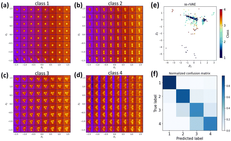
Hence, we applied the ss-rVAE to the GNPs dataset. In this case, the training is semi-supervised and the classification is performed via the y-encoder by encoding the data into a discrete latent variable. Then, other information, such as particle size and background signal intensity, is encoded into the standard continuous latent variables that contain information on physical factors of variability in data. The class-conditioned continuous latent spaces shown in Fig. 6a–d indicate good performance of ss-rVAE in the classification task as well as in discovering the main factors of variation for the images associated with each individual class. Indeed, both particle number and particle shapes are well identified in the latent space of the first three classes (Fig. 6a–c). The blurring of the latent space for the fourth class is due to the large number of possible configurations and (very) small numbers of examples. We also observe a variation of particle size and background information, suggesting that the physical meaning of the conventional latent variables is related to the particle size and background. Fig. 6f shows the confusion matrix of ss-rVAE on the nanoparticle dataset and the accuracy is higher than 0.6 for each class. The existing machine learning, including decision tree classifier, random forest classifier and XGBoost classifier, on the nanoparticle dataset perform poorly in the classification task (Fig. S3†). The comparison of VAE, rVAE, and ss-rVAE clearly indicates the superior performance of the ss-rVAE.
Conclusion
To summarize, we have introduced a semi-supervised rotationally-invariant variational autoencoder (ss-rVAE) as a universal approach that allows generalizing from a small subset of labeled data with a weak orientational disorder to a large unlabeled dataset with a much stronger orientational disorder. This approach both allows recovering missing labels for a dataset and disentangling continuous factors of variation for each class. Finally, the classifier part of the trained ss-rVAE inherits the rotational (and translational) invariances and can be deployed independently of the other parts of the model. The performance of the ss-rVAE was illustrated using synthetic data sets with the known factors of variation and was further extended to experimental data sets of clusters of gold nanoparticles. Hence, this approach provides a universal framework for the analysis of imaging data in areas as diversified as biology, medicine, condensed matter physics and materials science, and techniques ranging from optical to electron and scanning probe microscopies. In particular, it directly maps the common situation when small amounts of labeled data are available, in the form of prior published results, image collections and catalogs, or even theoretical models. It also can significantly reduce the need for labeled data. Finally, we note that VAE approach is naturally extendable for defining complex physical phenomena such as causal relationships (in the form of directed acyclic graphs connecting latent variables), topological structure of the data (via invariances of the latent space), opening the pathway towards exploring these phenomena based on observational data.Data availability
The detailed methodologies of semi-supervised rotationally-invariant variational autoencoder (ss-rVAE) on both synthetic and experimental datasets are established in Jupyter Notebooks and are available from https://github.com/ziatdinovmax/Semi-Supervised-VAE-nanoparticles. The source code for (ss-)rVAE is available via the pyroVED software package for invariant representation learning from imaging and spectral data: https://github.com/ziatdinovmax/pyroVED.Author contributions
D. S. G., M. Z. and S. V. K. conceived the project. M. Z. created the semi-supervised rotationally invariant variational autoencoder workflow and wrote the software enabling the analysis described in the paper. M. Y. Y. made the samples and collected the SEM data. Y. L., M. Y. Y., and S. V. K. performed detailed analyses with codes from M. Z. The manuscript was written with the contributions of all authors. All authors have given approval to the final version of the manuscript.Conflicts of interest
The authors declare no competing interests.Acknowledgements
This work was supported (M. Y. Y., D. G., S. V. K.) by the US Department of Energy, Office of Science, Office of Basic Energy Sciences, as part of the Energy Frontier Research Centers program: CSSAS – The Center for the Science of Synthesis Across Scales – under award number DE-SC0019288, located at University of Washington. SEM imaging was conducted at the University of Washington Molecular Analysis Facility, a National Nanotechnology Coordinated Infrastructure (NNCI) site which is supported in part by the National Science Foundation, the University of Washington, the Molecular Engineering and Sciences Institute, and the Clean Energy Institute. D. S. G. acknowledges support from the University of Washington, Department of Chemistry Kwiram Endowment. The ML of experimental data is supported (Y. L.) by the U.S. Department of Energy, Office of Science, Office of Basic Energy Sciences Energy Frontier Research Centers program under award number DE-SC0021118. The development and maintenance of the pyroVED software is supported (M. Z.) by the Laboratory Directed Research and Development Program at Pacific Northwest National Laboratory, a multiprogram national laboratory operated by Battelle for the U.S. Department of Energy. The authors acknowledge Dr Ilia Ivanov (CNMS) for early ideas (∼2010) of creating nanoparticle libraries.References
- S. V Kalinin, B. G. Sumpter and R. K. Archibald, Nat. Mater., 2015, 14, 973–980 CrossRef PubMed.
- S. V Kalinin, E. Strelcov, A. Belianinov, S. Somnath, R. K. Vasudevan, E. J. Lingerfelt, R. K. Archibald, C. Chen, R. Proksch, N. Laanait and S. Jesse, ACS Nano, 2016, 10, 9068–9086 CrossRef PubMed.
- B. G. Sumpter, R. K. Vasudevan, T. Potok and S. V Kalinin, npj Comput. Mater., 2015, 1, 15008 CrossRef CAS.
- A. Belianinov, R. Vasudevan, E. Strelcov, C. Steed, S. M. Yang, A. Tselev, S. Jesse, M. Biegalski, G. Shipman, C. Symons, A. Borisevich, R. Archibald and S. Kalinin, Adv. Struct. Chem. Imaging, 2015, 1, 6 CrossRef PubMed.
- F. Cichos, K. Gustavsson, B. Mehlig and G. Volpe, Nat. Mach. Intell., 2020, 2, 94–103 CrossRef.
- H. Chen, O. Engkvist, Y. Wang, M. Olivecrona and T. Blaschke, Drug Discovery Today, 2018, 23, 1241–1250 CrossRef PubMed.
- F. Jiang, Y. Jiang, H. Zhi, Y. Dong, H. Li, S. Ma, Y. Wang, Q. Dong, H. Shen and Y. Wang, Stroke Vasc. Neurol., 2017, 2, 230 CrossRef PubMed.
- M. A. Boles, M. Engel and D. V Talapin, Chem. Rev., 2016, 116, 11220–11289 CrossRef CAS PubMed.
- K. Kimura, K. Kobayashi, K. Matsushige and H. Yamada, Ultramicroscopy, 2013, 133, 41–49 CrossRef CAS PubMed.
- M. R. Hauwiller, X. Zhang, W.-I. Liang, C.-H. Chiu, Q. Zhang, W. Zheng, C. Ophus, E. M. Chan, C. Czarnik, M. Pan, F. M. Ross, W.-W. Wu, Y.-H. Chu, M. Asta, P. W. Voorhees, A. P. Alivisatos and H. Zheng, Nano Lett., 2018, 18, 6427–6433 CrossRef CAS PubMed.
- M. P. Oxley, J. Yin, N. Borodinov, S. Somnath, M. Ziatdinov, A. R. Lupini, S. Jesse, R. K. Vasudevan and S. V Kalinin, Mach. Learn.: Sci. Technol., 2020, 1, 04LT01 Search PubMed.
- F. Wu and N. Yao, Nano Energy, 2015, 11, 196–210 CrossRef CAS.
- H.-P. Komsa, J. Kotakoski, S. Kurasch, O. Lehtinen, U. Kaiser and A. V Krasheninnikov, Phys. Rev. Lett., 2012, 109, 35503 CrossRef PubMed.
- D. A. Bonnell and J. Garra, Rep. Prog. Phys., 2008, 71, 044501 CrossRef.
- C.-H. Lee, A. Khan, D. Luo, T. P. Santos, C. Shi, B. E. Janicek, S. Kang, W. Zhu, N. A. Sobh, A. Schleife, B. K. Clark and P. Y. Huang, Nano Lett., 2020, 20, 3369–3377 CrossRef CAS PubMed.
- A. Maksov, O. Dyck, K. Wang, K. Xiao, D. B. Geohegan, B. G. Sumpter, R. K. Vasudevan, S. Jesse, S. V Kalinin and M. Ziatdinov, npj Comput. Mater., 2019, 5, 12 CrossRef.
- S. V Kalinin, O. Dyck, S. Jesse and M. Ziatdinov, Sci. Adv., 2021, 7, eabd5084 CrossRef PubMed.
- L. Vlcek, A. Maksov, M. Pan, R. K. Vasudevan and S. V Kalinin, ACS Nano, 2017, 11, 10313–10320 CrossRef CAS PubMed.
- L. Vlcek, M. Ziatdinov, A. Maksov, A. Tselev, A. P. Baddorf, S. V Kalinin and R. K. Vasudevan, ACS Nano, 2019, 13, 718–727 CrossRef CAS PubMed.
- S. Wang and R. M. Summers, Med. Image Anal., 2012, 16, 933–951 CrossRef PubMed.
- M. Bosman, M. Watanabe, D. T. L. Alexander and V. J. Keast, Ultramicroscopy, 2006, 106, 1024–1032 CrossRef CAS PubMed.
- C. Ophus, Microsc. Microanal., 2019, 25, 563–582 CrossRef CAS PubMed.
- A. Chowdhury, E. Kautz, B. Yener and D. Lewis, Comput. Mater. Sci., 2016, 123, 176–187 CrossRef.
- M. H. Modarres, R. Aversa, S. Cozzini, R. Ciancio, A. Leto and G. P. Brandino, Sci. Rep., 2017, 7, 13282 CrossRef PubMed.
- Q. Luo, E. A. Holm and C. Wang, Nanoscale Adv., 2021, 3, 206–213 RSC.
- S. Akers, E. Kautz, A. Trevino-Gavito, M. Olszta, B. E. Matthews, L. Wang, Y. Du and S. R. Spurgeon, npj Comput. Mater., 2021, 7, 187 CrossRef CAS.
- J. Madsen, P. Liu, J. Kling, J. B. Wagner, T. W. Hansen, O. Winther and J. Schiøtz, Adv. Theory Simul., 2018, 1, 1800037 CrossRef.
- W. Li, K. G. Field and D. Morgan, npj Comput. Mater., 2018, 4, 36 CrossRef.
- Y. Han, Y. Liu, B. Wang, Q. Chen, L. Song, L. Tong, C. Lai and A. Konagaya, Neural Comput. Appl., 2022, 34, 5729–5741 CrossRef.
- E. Z. Qu, A. M. Jimenez, S. K. Kumar and K. Zhang, Macromolecules, 2021, 54, 3034–3040 CrossRef CAS.
- Y. Han, R. Li, S. Yang, Q. Chen, B. Wang and Y. Liu, Sci. Rep., 2022, 12, 12960 CrossRef CAS PubMed.
- C. K. Groschner, C. Choi and M. C. Scott, Microsc. Microanal., 2021, 27, 549–556 CrossRef CAS PubMed.
- S. Tsopanidis, R. H. Moreno and S. Osovski, Eng. Fract. Mech., 2020, 231, 106992 CrossRef.
- O. Furat, M. Wang, M. Neumann, L. Petrich, M. Weber, C. E. Krill and V. Schmidt, Front. Mater., 2019, 6, 145 CrossRef.
- Z. Yang, X. Li, L. Catherine Brinson, A. N. Choudhary, W. Chen and A. Agrawal, ASME J. Mech. Des., 2018, 140(11), 111416 CrossRef.
- Y. LeCun, Y. Bengio and G. Hinton, Nature, 2015, 521, 436–444 CrossRef CAS PubMed.
- J. E. van Engelen and H. H. Hoos, Mach. Learn., 2020, 109, 373–440 CrossRef.
- I. Gulrajani and D. Lopez-Paz, arXiv, 2020, preprint, arXiv:2007.01434, DOI:10.48550/arXiv.2007.01434.
- D. P. Kingma and M. Welling, Foundations and Trends® in Machine Learning, 2019, vol. 12, pp. 307–392 Search PubMed.
- D. P. Kingma and M. Welling, arXiv, 2013, preprint, arXiv:1312.6114, DOI:10.48550/arXiv.1312.6114.
- L. Deng, IEEE Signal Process. Mag., 2012, 29, 141–142 Search PubMed.
- T. Bepler, E. Zhong, K. Kelley, E. Brignole and B. Berger, in Advances in Neural Information Processing Systems, ed. H. Wallach, H. Larochelle, A. Beygelzimer, F. d'Alché-Buc, E. Fox and R. Garnett, Curran Associates, Inc., 2019, vol. 32 Search PubMed.
- D. Hernandez-Stumpfhauser, F. J. Breidt and M. J. van der Woerd, Bayesian Anal., 2017, 12, 113–133 Search PubMed.
- D. P. Kingma, D. J. Rezende, S. Mohamed and M. Welling, arXiv, 2014, preprint, arXiv:1406.5298, DOI:10.48550/arXiv.1406.5298.
- M. Ziatdinov and S. Kalinin, arXiv, 2021, preprint, arXiv:2104.10180, DOI:10.48550/arXiv.2104.10180.
Footnote |
| † Electronic supplementary information (ESI) available. See DOI: https://doi.org/10.1039/d3dd00196b |
| This journal is © The Royal Society of Chemistry 2024 |

