
 Open Access Article
 This Open Access Article is licensed under a
 Creative Commons Attribution 3.0 Unported Licence
Structural descriptors and information extraction from X-ray emission spectra: aqueous sulfuric acid†
E. A.
Eronen
 *a,
A.
Vladyka
a,
Ch. J.
Sahle
b and
J.
Niskanen
*a
*a,
A.
Vladyka
a,
Ch. J.
Sahle
b and
J.
Niskanen
*a
aDepartment of Physics and Astronomy, University of Turku, FI-20014 Turun yliopisto, Finland. E-mail: eemeli.a.eronen@utu.fi; johannes.niskanen@utu.fi
bESRF, The European Synchrotron, 71 Avenue des Martyrs, CS40220, 38043 Grenoble Cedex 9, France
First published on 15th August 2024
Abstract
Machine learning can reveal new insights into X-ray spectroscopy of liquids when the local atomistic environment is presented to the model in a suitable way. Many unique structural descriptor families have been developed for this purpose. We benchmark the performance of six different descriptor families using a computational data set of 24![[thin space (1/6-em)]](https://www.rsc.org/images/entities/char_2009.gif) 200 sulfur Kβ X-ray emission spectra of aqueous sulfuric acid simulated at six different concentrations. We train a feed-forward neural network to predict the spectra from the corresponding descriptor vectors and find that the local many-body tensor representation, smooth overlap of atomic positions and atom-centered symmetry functions excel in this comparison. We found a similar hierarchy when applying the emulator-based component analysis to identify and separate the spectrally relevant structural characteristics from the irrelevant ones. In this case, the spectra were dominantly dependent on the concentration of the system, whereas adding the second most significant degree of freedom in the decomposition allowed for distinction of the protonation state of the acid molecule.
200 sulfur Kβ X-ray emission spectra of aqueous sulfuric acid simulated at six different concentrations. We train a feed-forward neural network to predict the spectra from the corresponding descriptor vectors and find that the local many-body tensor representation, smooth overlap of atomic positions and atom-centered symmetry functions excel in this comparison. We found a similar hierarchy when applying the emulator-based component analysis to identify and separate the spectrally relevant structural characteristics from the irrelevant ones. In this case, the spectra were dominantly dependent on the concentration of the system, whereas adding the second most significant degree of freedom in the decomposition allowed for distinction of the protonation state of the acid molecule.
I. Introduction
The liquid phase allows for the movement of solvent and solute molecules while simultaneously having strong interactions among them. This leads to a distribution of possible local structures, and respective local electronic Hamiltonians. Computations have shown that these local environments yield significantly different X-ray spectra, while their ensemble mean is needed for a match with the corresponding experiment.1–8 Thus the changes in the experimental spectrum can be connected to corresponding changes in the local structural distribution. However, the complexity of this problem calls for sophisticated methods able to distinguish between relevant and irrelevant information. Recent developments in computational resources and machine learning (ML) have opened new paths for these investigations.9–17Because raw atomic coordinates R are unsuitable for contemporary ML, numerous families of descriptors D(R) have been developed to encode the structural information into a useful input.18–31 While each of these representations might perform well for some tasks, they are not necessarily equally fit for every situation. Beside the ML performance, interpretability of the descriptor is a key consideration for studies of actual structural information content of, e.g. X-ray spectra.17 The study of the spectrum-to-structure inverse problem is indeed highly dependent on the descriptor, which needs to include physically relevant features that are meaningful not only to ML models but also to human researchers.
Spectrum prediction by ML, i.e. finding a suitable function for spectrum S(D(R)), is a more viable task than structure prediction (finding function R(S)),13 possibly because the former is not an injective function. Moreover, some structural characteristics of the system are spectrally irrelevant. While the behavior of a spectrum can be captured by a well-performing feed-forward neural network (NN), the knowledge remains hidden in the respective weight matrices and bias vectors. To this end, the NN is useful only for predicting the outcome for new input, i.e. for emulation. Emulator-based component analysis (ECA)14 is an approach to extract knowledge contained by a ML model and a given data set. With the help of a fast emulator such as an NN, the method iteratively finds the structural dimensionality reduction for maximal explained spectral variance. The resulting basis vectors provide an exhaustive input feature selection, which not only points out spectrally relevant ones but also their collaborative effect.17 Moreover, approximate structural reconstruction from spectra can be done by first reconstructing the few spectrally dominant latent coordinates, and then taking an expansion with the respective basis vectors.16 Our previous work on N K-edge X-ray absorption spectroscopy of aqueous triglycine17 showed that ECA greatly outperforms principal component analysis (PCA)32 of structural data in terms of covered spectral variance. Furthermore, a recent study using encoder–decoder neural networks supports the validity of ECA.33 While the advantage of this method is its lack of need for any prior hypothesis, it gives rise to another requirement for a descriptor: decomposability into a few dominant contributions.17
We explore structural information content of simulated sulfur Kβ X-ray emission spectra (XES) of aqueous sulfuric acid. To create the data set we sample atomistic local structures from ab initio molecular dynamics (AIMD) simulations at six different concentrations and calculate spectra for these structures. We first assess a total of six structural descriptor families in terms of spectrum prediction performance by an NN. For a fair comparison between the descriptor families, we allocate equal computational resources to the joint hyperparameter–NN architecture search for each of them. Next, we identify the spectrally dominant structural degrees of freedom using ECA, and study the performance of the best descriptor of each family in the task. A sulfuric acid molecule can exist in one of three protonation states, which we find to be distinguishable from the XES after rank-two decomposition, in which the first rank covers intermolecular interaction given by the concentration. Our results highlight the need for identification of relevant structural degrees of freedom for reliable interpretation of X-ray spectra. Moreover, they raise a call for methods of obtaining simple structural information from contemporary structural descriptors, that may have a notably abstract mathematical form.
II. Methods
We base the study on structure–spectrum data pairs obtained from AIMD simulations and subsequent spectrum calculations resulting in 24200 data points. We encode the structural data using six different descriptor families and study the resulting performance of ML and subsequent ECA.
A. Simulations
We extended the AIMD runs of ref. 34 for structural sampling from six concentrations. The details of the AIMD runs are presented in Table 1. The simulations for the NVT ensemble were run using the CP2K software35 and Kohn–Sham density functional theory (DFT) with Perdew–Burke–Ernzerhof (PBE) exchange correlation potential.36 The AIMD runs utilized periodic boundary conditions, Goedecker–Teter–Hutter (GTH) pseudopotentials37–39 and triple-ξ TZVP-GTH basis set delivered with the software.| Num. conc. | Molarity [M] | Box L [Å] | Duration [ps] | Sampling [fs] | N snapshots | N spectra | SO42− [%] | HSO41− [%] | H2SO4 [%] |
|---|---|---|---|---|---|---|---|---|---|
| 1v63 | 0.9 | 12.50 | 100 | 62.5 | 1600 | 1600 | 96.2 | 3.8 | 0.0 |
| 6v54 | 4.9 | 12.66 | 50 | 62.5 | 800 | 4800 | 71.4 | 28.5 | 0.1 |
| 12v36 | 10.1 | 12.55 | 50 | 125 | 400 | 4800 | 17.2 | 79.3 | 3.5 |
| 20v20 | 15.3 | 12.95 | 50 | 250 | 200 | 4000 | 2.0 | 74.8 | 23.1 |
| 21v7 | 17.5 | 12.58 | 50 | 250 | 200 | 4200 | 0.0 | 28.7 | 70.8 |
| 24v0 | 18.6 | 12.90 | 50 | 250 | 200 | 4800 | 0.0 | 0.0 | 99.6 |
| Total | 24200 |
We computed the XES for every sulfur site of each sampled snapshot using the projector-augmented-wave (PAW) method40 with plane wave basis and density functional theory (DFT) implemented in GPAW version 22.1.0.40–42 We used periodic boundary conditions, the PBE exchange correlation potential and a 600 eV plane wave energy cutoff (for justification, see ESI†).
The spectrum calculations applied transition potential DFT43 in a fashion motivated in ref. 44. First, we computed the neutral ground state of each snapshot and emission lines for each site on a relative energy scale. We then calibrated the individual spectra on the absolute energy scale by a Δ-DFT calculation for the highest transition. This procedure builds on calculation with one valence vacancy and on respective calculations for the full core hole at each site, repeated for each snapshot. We convoluted the obtained energy–intensity pairs (a stick spectrum) with a Gaussian of full width at half maximum of 1.5 eV and then presented the spectra on a grid with bin width of 0.075 eV.
B. Data preprocessing
For ML and further analysis, we took the portion with notable spectral intensity around the peak group Kβx, Kβ1,3, and Kβ′′ (see Fig. 1 and e.g. ref. 45), and coarsened it by integration to a new grid with bin width of 0.75 eV leading to target spectra S represented as vectors of 16 components. We chose this grid to be as coarse as possible while still containing the relevant spectral features due to three reasons: (i) the fewer output values simplify the ML problem; (ii) individual data points are more independent without significant loss of information; (iii) we hope to avoid over-interpretation through overly detailed analysis of simulations.13 The last point follows the principle of correspondence i.e. analyzing simulations only to a degree in which they reproduce the experiment. | ||
| Fig. 1 Simulation results of aqueous sulfuric acid. (a) and (b) Two sample structures for 0.9 M and 15.3 M, respectively, prepared with the Jmol software.46 Only molecules within 3 Å distance from the central molecule are shown for clarity. (c) and (d) Computational ensemble mean X-ray emission spectrum for each concentration with the standard deviation σ shown as grey shaded area. As an example we show the location of the features Kβx, Kβ1,3 and Kβ′′45 for the highest concentration spectrum in panel (d). In addition, the coarsened grid points used for the target spectra of the machine-learning-based analysis are shown on the mean spectra. | ||
We evaluated the protonation state of each acid molecule as in ref. 34. An oxygen atom was considered to belong to the molecule if it was at most 2.0 Å from the respective sulfur atom. A hydrogen atom, in turn, was considered a part of the acid molecule if it was closer than 1.3 Å from any of its oxygen atoms. Throughout the simulations, the acid molecules always had four oxygen atoms with the distribution of forms: 5878 SO42−, 9435 HSO4−, 8847 H2SO4, and 40 H3SO4+ corresponding to protonations states from 0 to 3, respectively.
In this work we study six different descriptor families for encoding the local atomistic structure R around the emission site Sem into a vector of features D(R). We used the implementation within the DScribe-package (version 2.0.1)19,47 for the local version of the many-body tensor representation (LMBTR),20 smooth overlap of atomic positions (SOAP)22 and atom-centered symmetry functions (ACSF).21 For the many-body distribution functionals (MBDF)30 we used the implementation provided with the original publication. In addition, we implemented the descriptor introduced in ref. 28 calling it “Gaussian tensors” (GT) hereafter. Finally, we used a sorted variant of the Coulomb matrix (CM)23 similar to the bag of bonds24 and analogous to the implementation in ref. 16. We used the emission site Sem as the only center for building the descriptors LMBTR, SOAP, ACSF and GT.
We split the data set randomly to 80% (19360 data points) for the training, and the rest 20% (4840 data points) for testing. We calculated feature-wise z-score standardization for the obtained raw D(R) (NN input) and S (NN output) features using the training set and then applied this scaling to all data prior to any further procedures. The applied feature scaling is common practice in ML in general,48 and also in MD with atomic ML potentials in particular.49 Furthermore, it can be shown that the standardization does not limit the emulation performance of an NN, but is still essential for achieving unbiased L2 regularization during training (see ESI†).
C. Data analysis
Successful emulation requires model selection of the hyperparameters of the NN, and also those of the descriptor family. For example, there is no single LMBTR descriptor, but the numerous internal hyperparameters of this family are subject to model selection for optimal performance. Moreover, different descriptor hyperparametrizations (e.g. those within LMBTR) require different NN hyperparameters for optimal performance of the structure–spectrum emulator system. We carried out a joint search for these two hyperparametrizations in a randomized grid search for each descriptor family separately, allocating equal computational time for each search. In each case we used the best found descriptor–NN system for all subsequent analyses.We used fully connected feed-forward NNs implemented in PyTorch (version 2.0.1)50 for ML. This NN architecture allows for a range of possible hyperparameters that we searched over: the weight decay term α (from 10−13 to 1), number of hidden layers (2, 3, 4 or 5), hidden layer width (16, 32, 64, 128 or 256 neurons) and the learning rate (0.0001 or 0.00025). As the activation function of the neurons, we used the exponential linear unit (ELU).51 The training of the networks was done in mini-batches of 200 data points by maximizing the R2 score (coefficient of determination; generalized covered variance) using the Adam optimizer.52 We applied early stopping of the training by checking every 200 epochs if the validation score no longer improved.
We calculated the average score from a five-fold cross-validation (CV) on the training set for each selected descriptor–NN hyperparameter combination. Because building the descriptor consumed significantly more computational resources than training one NN model, we trained ten different NN architectures for every single descriptor hyperparametrization. The same procedure was repeated for each of the six descriptor families with equal total processor (CPU) time of the random grid search by allocating a total of 1440 CPU hours per descriptor family on Intel Xeon Gold 6230 processors at Puhti cluster computer, CSC, Finland. Different descriptor families have different free parameters to search over, which is detailed in the ESI.† We found slight variation of the results to persist within the searched grid space due to randomness, for example, in shuffling of the mini-batches and initialization of NN weights. In the end, we chose the descriptor–NN hyperparameters with the highest CV score and trained the final model using the full training set. In this final training we used 80% of re-shuffled training data (15488 points) for actual training and the rest 20% (3872 points) for validation to determine the early stopping condition.
We carried out ECA decomposition14 of the structural descriptor space using the PyTorch implementation of the algorithm.53 In the ECA procedure, basis vectors V = {vj}kj=1 are searched for to achieve a rank-k approximation for D(R):
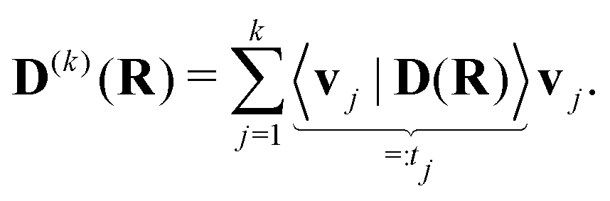 | (1) |
We found that the randomly selected initial guess of the ECA component vectors sometimes affected the resulting fit. Therefore, we ran the ECA procedure with 25 different random initial guesses for each component and always chose the vector resulting in the highest R2 score, before moving on to optimizing the next component. This is likely a symptom of the high-dimensional feature vectors, which encode a wealth of atomistic information within each (correlated) element of the vector. This complexity is inherited from the physical problem itself.
We used the training set for both NN training and ECA decomposition. The generalizability of the outcome was assessed with the test set in both cases. To allow for apples-to-apples comparison, we used the R2 score for all NN training, testing, and ECA.
III. Results
Sulfuric acid exists in different protonation states as exemplified by sample structures in Fig. 1a and b showing local structures from simulations of 0.9 M and 15.3 M solutions. The simulated ensemble average spectra of different concentrations are shown in Fig. 1c and d. There is a clear concentration dependency around the Kβx–Kβ1,3–Kβ′′ line group, where the central peak shows a decreasing trend, and the Kβx and Kβ′′ an increasing one, along the concentration. Additionally, our simulated spectra show shifts in energy. The general shape of the spectra match well with the experiment published in ref. 5 and, therefore, the data set can be considered suitable for the ML and subsequent analysis of this work. The chosen region and coarsened bins of the target spectra (depicted with points in Fig. 1c and d) are sufficient to capture the shape of the spectrum.Even after extensive model selection, the descriptors yield varying prediction performance of the target spectra as presented in Table 2. Practically equal accuracy is obtained with the best-performing descriptors LMBTR, SOAP and ACSF. The MBDF descriptor provides intermediate performance among the studied ones, whereas GT and CM yield more than 0.1 units lower R2 than the most accurate descriptors. The tendency of an ML model to overfit is commonly measured by the difference between the train and the test scores. Our results hint an increasing trend in this difference along decreasing accuracy. Fig. 2a illustrates the distribution of the R2 scores for z-score inverse transformed (absolute intensity) spectral features using the LMBTR emulator with an overall test set R2 of 0.950. Additionally, typical prediction quality along this distribution is presented in Fig. 2b–d. A similar figure for the z-score-standardized spectral space with R2 of 0.928 is available in the ESI.†
| Descriptor | N features | R train 2 | R test 2 | Difference |
|---|---|---|---|---|
| LMBTR | 420 | 0.944 | 0.928 | 0.015 |
| SOAP | 2700 | 0.961 | 0.928 | 0.033 |
| ACSF | 543 | 0.952 | 0.923 | 0.029 |
| MBDF | 330 | 0.915 | 0.878 | 0.036 |
| GT | 1275 | 0.857 | 0.814 | 0.043 |
| CM | 595 | 0.889 | 0.806 | 0.083 |
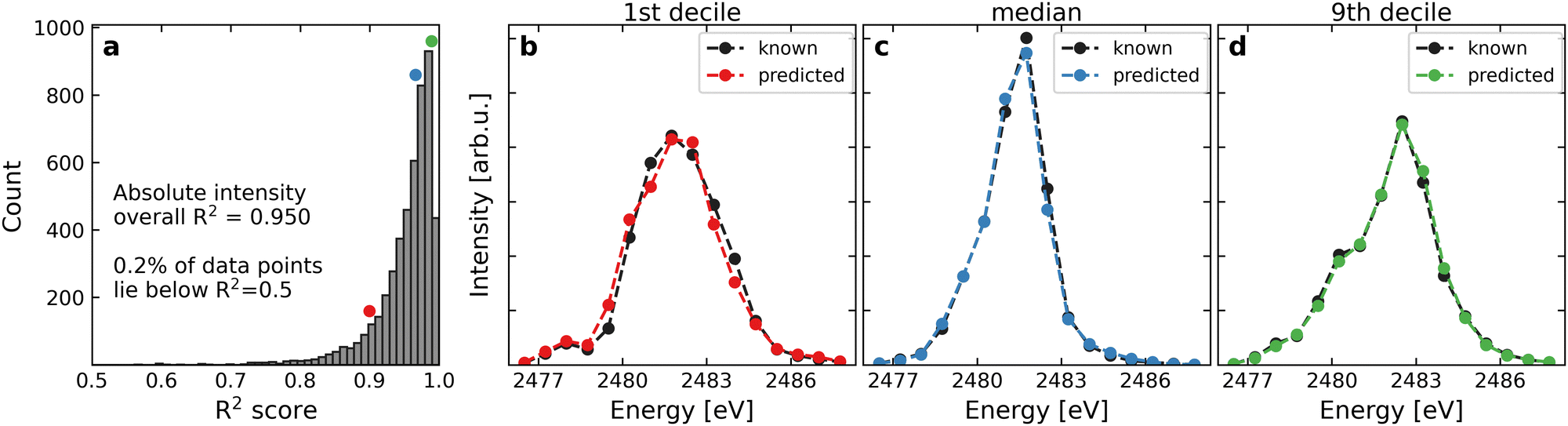 | ||
| Fig. 2 Absolute intensity scale spectrum prediction performance of the best NN-LMBTR model measured using the test set. (a) Distribution of R2 scores for each data point. Examples of known and predicted spectra with R2 score closest to (b) the 1st decile, (c) the median, and (d) the 9th decile. For each of the three cases, the location along the R2 distribution is shown in panel a as a correspondingly colored circle. The scores of this figure differ from the rest of the study as ML was applied to z-score standardized spectra. For a similar plot using the standardized spectra, see ESI.† | ||
We measure the ECA decomposition performance with the R2 score, shown as a function of the rank of the decomposition in Fig. 3. The scores for the train set and for the test set both rise monotonically and approach a plateau near the respective emulator performance. In general, the R2 scores of high rank (≥5) ECA are roughly ordered along the overall ML accuracy of the respective emulators. The design principle of ECA aims at maximal covered spectral variance at any given rank, manifested by the diminishing improvement as a function of k observed in Fig. 3. Consequently, the high-k scores tk are not reconstructable from the spectra, as these degrees of freedom are irrelevant in their emulation. With components of negligible effect on the outcome, full structural reconstruction from spectra is impossible, as a structural descriptor is completely defined by expansion (1) done to the full rank. The intended rapid reduction of dimensionality motivates the study of low rank (e.g. k ≤ 3) decompositions for which LMBTR performs the best. We have noticed jumps in the R2 curves as a function of the decomposition rank k, seen in Fig. 3 for SOAP and CM. This phenomenon is unpredictable and potentially related to the initial guess of the ECA component vector. Apart from the obvious complexity of the problem, the detailed origin and cure for this behaviour remain unknown to us.
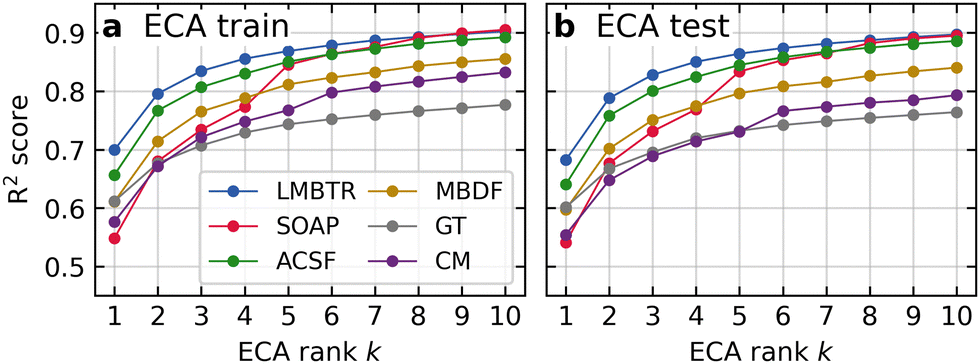 | ||
| Fig. 3 Typical behaviour of the (a) train and (b) test R2 score as a function of the ECA rank k for each descriptor after joint model selection of the representation and neural network architecture. Standardized output features are used. At high ranks the results closely follow those of the emulation performance. Increasing the rank shows diminishing R2-score gains. At low ranks LMBTR outperforms the rest. The jump observed SOAP and CM may occur for any descriptor and is due to the complexity of the problem and stochasticity of the iterative solution. | ||
Next, we analyse the ECA results using the LMBTR descriptor, which contains simple physical information as part of it, namely element-wise interatomic distances from the emission site Sem. Instead of presenting the numeric values of these distances, the descriptor encodes the information on a predefined grid as a sum of Gaussian functions, centered at the respective positions. The according features of the first ECA component vector, z-score inverse transformed into the descriptor space, are shown in Fig. 4a. In the sense of the aforementioned representation, these curves reflect the change in the interatomic distances most relevant in terms of the target spectrum shape. The figure shows that the S Kβ XES is affected by notably distant molecules. As the typical protonating H distance from the S atom of the acid molecule is 2.2 Å, the part corresponding to the Sem–H distribution shows notable relevance in the region above 3 Å. This can be attributed to the different hydrogen number density in the system reflecting the concentration, with possibly minor effects coming from hydrogen bonding of the system. The concentration dependency is further indicated by the opposite effect of Sem–S curve at 4–6 Å. Additionally, the Sem–H distribution shows a weaker effect in the region between 1 Å and 3 Å, which likely arises from the tails of the descriptor Gaussians corresponding to the hydrogen atoms protonating the acid molecule.
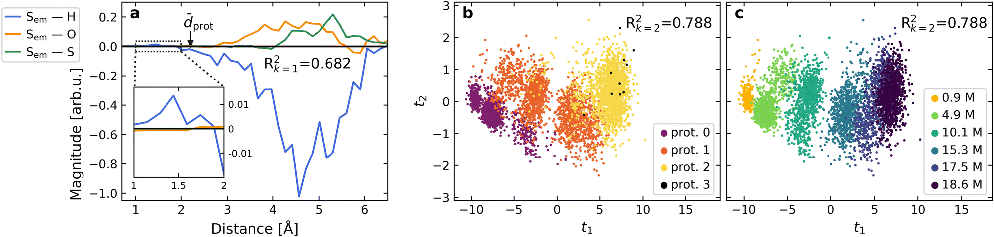 | ||
Fig. 4 Results of the ECA using the LMBTR descriptor. (a) Interatomic distance part of the first ECA vector (with spectral Rk=12 = 0.682) z-score inverse transformed into the descriptor space. A separate sub-panel shows the region between 1 Å and 2 Å. The non-zero values of the vector show that even distant atoms have a significant effect on the spectra. The arrow at ![[d with combining macron]](https://www.rsc.org/images/entities/i_char_0064_0304.gif) prot = 2.20 Å shows the mean distance to the hydrogen atoms protonating the acid molecule. (b) and (c) Two-dimensional ECA projection (with spectral Rk=22 = 0.788) of each data point in the test set: both of the components are necessary to distinguish the protonation state of the acid molecule, whereas the first component follows intermolecular interactions given by concentration. See text for details. prot = 2.20 Å shows the mean distance to the hydrogen atoms protonating the acid molecule. (b) and (c) Two-dimensional ECA projection (with spectral Rk=22 = 0.788) of each data point in the test set: both of the components are necessary to distinguish the protonation state of the acid molecule, whereas the first component follows intermolecular interactions given by concentration. See text for details. | ||
The first two ECA components correspond to structural features which define the majority of the spectral variance (Rk=12 = 0.682, Rk=22 = 0.788). Recent results indicate orders of magnitude better R2 score for covered spectral variance by ECA in comparison to that obtained by PCA for the structural descriptor.17 In the case of S Kβ XES of aqueous H2SO4 such a drastic difference is not observed: here a 2-component structural decomposition by PCA resulted in R2 = 0.453 for spectral variance, which is still notably less than the Rk=22 = 0.788 obtained by ECA. This indicates a more direct structural characteristics – spectral response relation in the current case.
To study the separability of spectrally dominant structural features, we performed projection of each data point in the test set on two-dimensional ECA space. We focus on two most obvious characteristics: the protonation state of an acid molecule and the concentration of the system, which are indicated by coloring of each point in the resulting scatter plot, shown in Fig. 4b and c, respectively. The protonation state is not the ruling structural characteristic behind variation of the S Kβ XES as it can be only partially identified by the first ECA score t1 (Fig. 4b). However, the interplay of t1 and t2 disentangles these classes almost completely. This result is supported by the fact that the first component vector shows only a weak effect in Fig. 4a along the part of the curve which corresponds to the protonating hydrogen atoms. In contrast, the score t1 describes the concentration of the system, seen as the spectral change in Fig. 1c and d and in our analysis of the respective Sem–H curve in Fig. 4a. Ultimately, the need for the second degree of freedom to identify the protonation state is congruent with the overlap between the spectral-region intensity histograms of the protonation states, reported in a previous work on aqueous H2SO4.5
IV. Discussion
The role of the descriptor is to present the structural data in the most utilizable form for emulation, for which numerous studies have been published in the context of atomistic systems.15,54–56 These comparisons indicate that the optimal choice of the descriptor family depends on the application, and probably on the system. For example, in prediction of the X-ray absorption near edge structure (XANES) of amorphous carbon Kwon et al.15 found LMBTR to perform best (ACSF, LMBTR and SOAP studied). However, spectral neighbor analysis potential (SNAP)25,26 outperformed for XANES of amorphous silicon glass in the work of Hirai et al.54 (ACSF, LMBTR, SNAP and SOAP studied). In an other context, SOAP was deemed most favorable by Onat et al.55 for potential energy prediction of silicon (atomic cluster expansion,27 ACSF, introduced Chebyshev polynomials in symmetry functions, MBTR, and SOAP studied). Interestingly, the same conclusion was drawn by Jäger et al.56 in prediction of hydrogen adsorption energies on nanoclusters (MBTR, SOAP and ACSF studied). We note that systematic, wide and blind hyperparameter searches appear rare in the literature. Moreover, the joint descriptor–NN hyperparameter search used in this work has further potential of improving performance of any descriptor family in such a comparison.Our results suggest that, in X-ray spectroscopy of liquids (with ≈2 × 10⁴ data points) an equal ML performance can be obtained with LMBTR, SOAP and ACSF with joint model selection of the descriptor hyperparameters together with the NN architecture. Among the studied descriptor families, we obtained intermediate performance with MBDF, whereas we could not achieve competitive accuracy when using CM and GT. The result thus highlights the need of suitable encoding of information by the descriptor. Although the CM can be even converted back to the original structure with the loss of only handedness of the system, and although the descriptor family performed quite well for Ge Kβ XES of amorphous GeO2,16 it does not excel with the current liquid system.
Picking a descriptor family poses a serious model selection problem because there are inherent tunable hyperparameters characteristic to each one of them (see ESI†). Due to expected interplay between the optimal NN architecture, this optimization is ideally done jointly with the hyperparameters of the NN, which multiplies the required computational effort. Without prior knowledge, descriptors with more free hyperparameters are more flexible than those with fewer. Therefore, their parameter-optimized forms have a higher prior potential for accuracy as well. Because this tuning is ultimately left for the user, we accounted for the discrepancy in descriptor design by applying equal computation time for refining each descriptor, regardless how many free hyperparameters the implementation had. We propose this practice for fair assessment of structural descriptors of ever-increasing multitude. Furthermore, we find that the top-level performance among the descriptor family is typically achieved with several drastically different parametrizations. Therefore we conclude that diminishing CV score gains provides a reasonable stopping condition for the joint randomized hyperparameter search, if the allowed hyperparameter space is sufficiently large.
In this work we chose to measure the performance using the R2 score, which is a widely applied metric for information captured by a model, and utilized in e.g. PCA. The score is well-suited for spectrum interpretation because it is independent of the units and of the absolute scale. The sulfur atom has a Kβ baseline spectrum in the SO4 moiety, and therefore respective variation evaluated by the R2 score yields an informative measure for interpretation of spectra. When using z-score standardized output, the R2 gives each output feature an equal importance in the spectral interpretation, whereas raw spectral intensity favors features of large variation, observed typically for features with large overall intensity. We motivate the choice of standardization by the nonlinearity of the structure–spectrum relationship. Namely, a weak spectral feature may be indicative of a more interesting or a more widely present structural characteristics than its absolute intensity might indicate. We note however, that the analysis methods applied in this work do not necessitate the use of either output standardization or the R2 score.
Analogous to PCA, ECA works as a dimensionality reduction tool. Instead of maximizing the covered structural variance, the method focuses on maximizing the spectral one for a decomposition in the structural space. As a result, the basis vectors of ECA can be used to identify descriptor features, which affect (or do not affect) the shape of the target spectra, or even for approximate structural reconstruction from spectra.16 The method is capable of a remarkable reduction of dimensionality,14,16,17 improving on similar methods such as the partial least squares fitting with singular value decomposition57 as demonstrated in ref. 14. The first ECA component vector, shown in Fig. 4a, represents the dominant structural effect behind the variation of the spectrum. Although higher-rank ECA components may have cancelling contributions to those of lower ranks, these refinements are not equally relevant for spectrum interpretation as manifested by the associated diminishing spectral effect. We also note that the overall sign of an ECA vector can be chosen arbitrarily (adjusting the sign of the according score), but the relative signs of its components (e.g. the curves in Fig. 4a) are always fixed.
Structural interpretation of spectra sets several requirements for a descriptor. The representation needs to allow for accurate emulation, effective decomposition, and back-conversion to simple physical information. Although all of the studied descriptors are calculated from local atomistic structures, several factors complicate recovering such information from them. These include smearing the exact values on a grid and summation of information from many atoms into one feature, possibly with distance-dependent weights. In addition, some of the descriptors rely on basis functions and may potentially have an abstract mathematical form. In this line of thought, interpretation of descriptors calls for future efforts.
Machine learning by NNs requires large data sets, that have only recently become feasible owing to the increase in computational resources and the developments in simulation tools. Advances of ML in potentials for molecular dynamics,49,58,59 and in electron structure calculations,60 could help generate more extensive and more accurate training data, leading to improved performance of spectrum emulation and subsequent analyses.
V. Conclusions
We benchmarked six structural descriptor families in machine learning of simulated X-ray emission spectra (XES) of aqueous sulfuric acid. For unbiased assessment of these descriptor types with varying number of hyperparameters, we allocated equal computation time for the joint descriptor–neural network model selection in each of the six cases. We found local many-body tensor representation (LMBTR), smooth overlap of atomic positions (SOAP) and atom-centered symmetry functions (ACSF) to perform best (equally accurately) with the data set of ∼2 × 10⁴ points.We observed a similar hierarchy in the comparison of the descriptor families for structural dimensionality reduction guided by covered spectral variance. The LMBTR stood out especially in the low-rank decompositions of the applied emulator-based component analysis. Although the system manifests significant complexity, the analysis method managed to condense spectral dependence into two dimensions with R2 = 0.788 for an independent test set. The results indicated that even distant atoms have a significant effect on the XES, that probes local bound orbitals around the emission site. The dominant underlying coordinate t1 followed the concentration of the system, whereas inclusion of the second most relevant degree of freedom t2 allowed for clear distinction of the protonation state of the acid molecule. Altogether, our results highlight loss of structural information upon formation of a spectrum, which will have implications for justified interpretation of spectra using simulations.
Structural descriptors facilitate accurate prediction of X-ray spectra by a neural network. Advances in simulation methods can be anticipated to extend and improve the data sets to allow for studies of even more complex systems and analyses with higher accuracy. Conversion of the descriptor back to simple atomistic information needs specific research efforts, as results presented in terms of these mathematically sophisticated representations can be difficult to interpret by a human.
Author contributions
E. A. E. machine learning, data analysis, writing the manuscript. A. V. simulations, data analysis, writing the manuscript. C. J. S. writing the manuscript. J. N. research design, simulations, funding, writing the manuscript.Data availability
The data and relevant scripts are available in Zenodo: https://zenodo.org/doi/10.5281/zenodo.10650121.Conflicts of interest
There are no conflicts to declare.Acknowledgements
E. A. E. acknowledges Jenny and Antti Wihuri Foundation for funding. E. A. E., A. V. and J. N. acknowledge Academy of Finland for funding via project 331234. The authors acknowledge CSC – IT Center for Science, Finland, and the FGCI – Finnish Grid and Cloud Infrastructure for computational resources.References
- P. Wernet, D. Nordlund, U. Bergmann, M. Cavalleri, M. Odelius, H. Ogasawara, L. Näslund, T. K. Hirsch, L. Ojamäe, P. Glatzel, L. G. M. Pettersson and A. Nilsson, The Structure of the First Coordination Shell in Liquid Water, Science, 2004, 3040(5673), 995–999, DOI:10.1126/science.1096205.
- M. Leetmaa, M. P. Ljungberg, A. Lyubartsev, A. Nilsson and L. G. M. Pettersson, Theoretical approximations to X-ray absorption spectroscopy of liquid water and ice, J. Electron Spectrosc. Relat. Phenom., 2010, 1770(2–3), 135–157, DOI:10.1016/j.elspec.2010.02.004.
- N. Ottosson, K. J. Børve, D. Spångberg, H. Bergersen, L. J. Sæthre, M. Faubel, W. Pokapanich, G. Öhrwall, O. Björneholm and B. Winter, On the Origins of Core-Electron Chemical Shifts of Small Biomolecules in Aqueous Solution: Insights from Photoemission and ab Initio Calculations of Glycineaq, J. Am. Chem. Soc., 2011, 1330(9), 3120–3130, DOI:10.1021/ja110321q.
- C. J. Sahle, C. Sternemann, C. Schmidt, S. Lehtola, S. Jahn, L. Simonelli, S. Huotari, M. Hakala, T. Pylkkänen, A. Nyrow, K. Mende, M. Tolan, K. Hämäläinen and M. Wilke, Microscopic structure of water at elevated pressures and temperatures, Proc. Natl. Acad. Sci. U. S. A., 2013, 1100(16), 6301–6306, DOI:10.1073/pnas.1220301110.
- J. Niskanen, Ch. J. Sahle, K. O. Ruotsalainen, H. Müller, M. Kavčič, M. Žitnik, K. Bučdar, M. Petric, M. Hakala and S. Huotari, Sulphur Kβ emission spectra reveal protonation states of aqueous sulfuric acid, Sci. Rep., 2016, 6, 21012, DOI:10.1038/srep21012.
- J. Niskanen, C. J. Sahle, K. Gilmore, F. Uhlig, J. Smiatek and A. Föhlisch, Disentangling Structural Information From Core-level Excitation Spectra, Phys. Rev. E, 2017, 96, 013319, DOI:10.1103/PhysRevE.96.013319.
- J. Niskanen, M. Fondell, Ch. J. Sahle, S. Eckert, R. M. Jay, K. Gilmore, A. Pietzsch, M. Dantz, X. Lu, D. McNally, T. Schmitt, V. Vaz da Cruz, V. Kimberg, F. Gelmukhanov and A. Föhlisch, Compatibility of quantitative X-ray spectroscopy with continuous distribution models of water at ambient conditions, Proc. Natl. Acad. Sci. U. S. A., 2019, 1160(10), 4058–4063, DOI:10.1073/pnas.1815701116.
- V. V. da Cruz, F. Gelmukhanov, S. Eckert, M. Iannuzzi, E. Ertan, A. Pietzsch, R. C. Couto, J. Niskanen, M. Fondell, M. Dantz, T. Schmitt, X. Lu, D. McNally, R. M. Jay, V. Kimberg, A. Föhlisch and M. Odelius, Probing hydrogen bond strength in liquid water by resonant inelastic X-ray scattering, Nat. Commun., 2019, 100(1), 1013, DOI:10.1038/s41467-019-08979-4.
- J. Timoshenko, D. Lu, Y. Lin and A. I. Frenkel, Supervised Machine-Learning-Based Determination of Three-Dimensional Structure of Metallic Nanoparticles, J. Phys. Chem. Lett., 2017, 80(20), 5091–5098, DOI:10.1021/acs.jpclett.7b02364.
- J. Timoshenko and A. I. Frenkel, “Inverting” X-ray Absorption Spectra of Catalysts by Machine Learning in Search for Activity Descriptors, ACS Catal., 2019, 90(11), 10192–10211, DOI:10.1021/acscatal.9b03599.
- Y. Liu, N. Marcella, J. Timoshenko, A. Halder, B. Yang, L. Kolipaka, M. J. Pellin, S. Seifert, S. Vajda, P. Liu and A. I. Frenkel, Mapping XANES spectra on structural descriptors of copper oxide clusters using supervised machine learning, J. Chem. Phys., 2019, 1510(16), 164201, DOI:10.1063/1.5126597.
- N. Andrejevic, J. Andrejevic, B. A. Bernevig, N. Regnault, F. Han, G. Fabbris, T. Nguyen, N. C. Drucker, C. H. Rycroft and M. Li, Machine-Learning Spectral Indicators of Topology, Adv. Mater., 2022, 340(49), 2204113, DOI:10.1002/adma.202204113.
- J. Niskanen, A. Vladyka, J. A. Kettunen and C. J. Sahle, Machine learning in interpretation of electronic core-level spectra, J. Electron Spectrosc. Relat. Phenom., 2022, 260, 147243, DOI:10.1016/j.elspec.2022.147243.
- J. Niskanen, A. Vladyka, J. Niemi and C. J. Sahle, Emulator-based decomposition for structural sensitivity of core-level spectra, R. Soc. Open Sci., 2022, 90(6), 220093, DOI:10.1098/rsos.220093.
- H. Kwon, W. Sun, T. Hsu, W. Jeong, F. Aydin, S. Sharma, F. Meng, M. R. Carbone, X. Chen, D. Lu, L. F. Wan, M. H. Nielsen and T. A. Pham, Harnessing Neural Networks for Elucidating X-ray Absorption Structure-Spectrum Relationships in Amorphous Carbon, J. Phys. Chem. C, 2023, 1270(33), 16473–16484, DOI:10.1021/acs.jpcc.3c02029.
- A. Vladyka, C. J. Sahle and J. Niskanen, Towards structural reconstruction from X-ray spectra, Phys. Chem. Chem. Phys., 2023, 250(9), 6707–6713, 10.1039/D2CP05420E.
- E. A. Eronen, A. Vladyka, F. Gerbon, C. J. Sahle and J. Niskanen, Information bottleneck in peptide conformation determination by x-ray absorption spectroscopy, J. Phys. Commun., 2024, 80(2), 025001, DOI:10.1088/2399-6528/ad1f73.
- J. Behler, Perspective: Machine learning potentials for atomistic simulations, J. Chem. Phys., 2016, 1450(17), 170901, DOI:10.1063/1.4966192.
- L. Himanen, M. O. J. Jäger, E. V. Morooka, F. F. Canova, Y. S. Ranawat, D. Z. Gao, P. Rinke and A. S. Foster, DScribe: Library of descriptors for machine learning in materials science, Comput. Phys. Commun., 2020, 247, 106949, DOI:10.1016/j.cpc.2019.106949.
- H. Huo and M. Rupp, Unified representation of molecules and crystals for machine learning, Mach. Learn.: Sci. Technol., 2022, 30(4), 045017, DOI:10.1088/2632-2153/aca005.
- J. Behler, Atom-centered symmetry functions for constructing high-dimensional neural network potentials, J. Chem. Phys., 2011, 1340(7), 074106, DOI:10.1063/1.3553717.
- A. P. Bartók, R. Kondor and G. Csányi, On representing chemical environments, Phys. Rev. B: Condens. Matter Mater. Phys., 2013, 87, 184115, DOI:10.1103/PhysRevB.87.184115.
- M. Rupp, A. Tkatchenko, K.-R. Müller and O. A. von Lilienfeld, Fast and Accurate Modeling of Molecular Atomization Energies with Machine Learning, Phys. Rev. Lett., 2012, 108, 058301, DOI:10.1103/PhysRevLett.108.058301.
- K. Hansen, F. Biegler, R. Ramakrishnan, W. Pronobis, O. A. von Lilienfeld, K.-R. Müller and A. Tkatchenko, Machine Learning Predictions of Molecular Properties: Accurate Many-Body Potentials and Nonlocality in Chemical Space, J. Phys. Chem. Lett., 2015, 60(12), 2326–2331, DOI:10.1021/acs.jpclett.5b00831.
- A. P. Thompson, L. P. Swiler, C. R. Trott, S. M. Foiles and G. J. Tucker, Spectral neighbor analysis method for automated generation of quantum-accurate interatomic potentials, J. Comput. Phys., 2015, 285, 316–330, DOI:10.1016/j.jcp.2014.12.018.
- M. A. Wood and A. P. Thompson, Extending the accuracy of the SNAP interatomic potential form, J. Chem. Phys., 2018, 1480(24), 241721, DOI:10.1063/1.5017641.
- R. Drautz, Atomic cluster expansion for accurate and transferable interatomic potentials, Phys. Rev. B, 2019, 99, 014104, DOI:10.1103/PhysRevB.99.014104.
- A. Chandrasekaran, D. Kamal, R. Batra, C. Kim, L. Chen and R. Ramprasad, Solving the electronic structure problem with machine learning, npj Comput. Mater., 2019, 50(1), 22, DOI:10.1038/s41524-019-0162-7.
- M. F. Langer, A. Goeßmann and M. Rupp, Representations of molecules and materials for interpolation of quantum-mechanical simulations via machine learning, npj Comput. Mater., 2022, 80(1), 41, DOI:10.1038/s41524-022-00721-x.
- D. Khan, S. Heinen and O. A. von Lilienfeld, Kernel based quantum machine learning at record rate: Many-body distribution functionals as compact representations, J. Chem. Phys., 2023, 1590(3), 034106, DOI:10.1063/5.0152215.
- C. Middleton, B. Curchod and T. Penfold, Partial Density of States Representation for Accurate Deep Neural Network Predictions of X-ray Spectra, ChemRxiv, 2024 DOI:10.26434/chemrxiv-2024-bbrgt.
- I. T. Jolliffe and J. Cadima, Principal component analysis: a review and recent developments, Philos. Trans. R. Soc., A, 2016, 3740(2065), 20150202, DOI:10.1098/rsta.2015.0202.
- J. Passilahti, A. Vladyka and J. Niskanen, Encoder-Decoder Neural Networks in Interpretation of X-ray Spectra, arXiv, 2024, preprint, arXiv:2406.14044v1 [physics.atm-clus] DOI:10.48550/arXiv.2406.14044.
- J. Niskanen, Ch. J. Sahle, I. Juurinen, J. Koskelo, S. Lehtola, R. Verbeni, H. Müller, M. Hakala and S. Huotari, Protonation dynamics and hydrogen Bonding in aqueous sulfuric acid, J. Phys. Chem. B, 2015, 1190(35), 11732, DOI:10.1021/acs.jpcb.5b04371.
- T. D. Kühne, M. Iannuzzi, M. Del Ben, V. V. Rybkin, P. Seewald, F. Stein, T. Laino, R. Z. Khaliullin, O. Schütt, F. Schiffmann, D. Golze, J. Wilhelm, S. Chulkov, M. H. Bani-Hashemian, V. Weber, U. Borštnik, M. Taillefumier, A. S. Jakobovits, A. Lazzaro, H. Pabst, T. Müller, R. Schade, M. Guidon, S. Andermatt, N. Holmberg, G. K. Schenter, A. Hehn, A. Bussy, F. Belleflamme, G. Tabacchi, A. Glöβ, M. Lass, I. Bethune, C. J. Mundy, C. Plessl, M. Watkins, J. VandeVondele, M. Krack and J. Hutter, CP2K: An electronic structure and molecular dynamics software package - Quickstep: Efficient and accurate electronic structure calculations, J. Chem. Phys., 2020, 1520(19), 194103, DOI:10.1063/5.0007045.
- J. P. Perdew, K. Burke and M. Ernzerhof, Generalized gradient approximation made simple, Phys. Rev. Lett., 1996, 77, 3865–3868, DOI:10.1103/PhysRevLett.77.3865.
- S. Goedecker, M. Teter and J. Hutter, Separable dual-space Gaussian pseudopotentials, Phys. Rev. B: Condens. Matter Mater. Phys., 1996, 54, 1703–1710, DOI:10.1103/PhysRevB.54.1703.
- C. Hartwigsen, S. Goedecker and J. Hutter, Relativistic separable dual-space Gaussian pseudopotentials from H to Rn, Phys. Rev. B: Condens. Matter Mater. Phys., 1998, 58, 3641–3662, DOI:10.1103/PhysRevB.58.3641.
- M. Krack, Pseudopotentials for H to Kr optimized for gradient-corrected exchange-correlation functionals, Theor. Chem. Acc., 2005, 1140(1), 145–152, DOI:10.1007/s00214-005-0655-y.
- J. Enkovaara, C. Rostgaard, J. J. Mortensen, J. Chen, M. Dułak, L. Ferrighi, J. Gavnholt, C. Glinsvad, V. Haikola, H. A. Hansen, H. H. Kristoffersen, M. Kuisma, A. H. Larsen, L. Lehtovaara, M. Ljungberg, O. Lopez-Acevedo, P. G. Moses, J. Ojanen, T. Olsen, V. Petzold, N. A. Romero, J. Stausholm-Møller, M. Strange, G. A. Tritsaris, M. Vanin, M. Walter, B. Hammer, H. Häkkinen, G. K. H. Madsen, R. M. Nieminen, J. K. Nørskov, M. Puska, T. T. Rantala, J. Schiøtz, K. S. Thygesen and K. W. Jacobsen, Electronic structure calculations with GPAW: a real-space implementation of the projector augmented-wave method, J. Phys.: Condens. Matter, 2010, 220(25), 253202, DOI:10.1088/0953-8984/22/25/253202.
- J. J. Mortensen, L. B. Hansen and K. W. Jacobsen, Real-space grid implementation of the projector augmented wave method, Phys. Rev. B: Condens. Matter Mater. Phys., 2005, 710(3), 035109, DOI:10.1103/PhysRevB.71.035109.
- A. H. Larsen, J. J. Mortensen, J. Blomqvist, I. E. Castelli, R. Christensen, M. Dułak, J. Friis, M. N. Groves, B. Hammer, C. Hargus, E. D. Hermes, P. C. Jennings, P. B. Jensen, J. Kermode, J. R. Kitchin, E. L. Kolsbjerg, J. Kubal, K. Kaasbjerg, S. Lysgaard, J. B. Maronsson, T. Maxson, T. Olsen, L. Pastewka, A. Peterson, C. Rostgaard, J. Schiøtz, O. Schütt, M. Strange, K. S. Thygesen, T. Vegge, L. Vilhelmsen, M. Walter, Z. Zeng and K. W. Jacobsen, The atomic simulation environment Python library for working with atoms, J. Phys.: Condens. Matter, 2017, 290(27), 273002, DOI:10.1088/1361-648X/aa680e.
- L. Triguero, L. G. M. Pettersson and H. Ågren, Calculations of near-edge x-ray-absorption spectra of gas-phase and chemisorbed molecules by means of density-functional and transition-potential theory, Phys. Rev. B: Condens. Matter Mater. Phys., 1998, 58, 8097–8110, DOI:10.1103/PhysRevB.58.8097.
- M. P. Ljungberg, J. J. Mortensen and L. G. M. Pettersson, An implementation of core level spectroscopies in a real space Projector Augmented Wave density functional theory code, J. Electron Spectrosc. Relat. Phenom., 2011, 1840(8), 427–439, DOI:10.1016/j.elspec.2011.05.004.
- R. Alonso Mori, E. Paris, G. Giuli, S. G. Eeckhout, M. Kavčič, M. Žitnik, K. Bučar, L. G. M. Pettersson and P. Glatzel, Sulfur-metal orbital hybridization in sulfur-bearing compounds studied by X-ray emission spectroscopy, Inorg. Chem., 2010, 490(14), 6468–6473, DOI:10.1021/ic100304z.
- Jmol development team. Jmol: an open-source Java viewer for chemical structures in 3D, https://www.jmol.org/.
- J. Laakso, L. Himanen, H. Homm, E. V. Morooka, M. O. J. Jäger, M. Todorovic and P. Rinke, Updates to the DScribe library: New descriptors and derivatives, J. Chem. Phys., 2023, 1580(23), 234802, DOI:10.1063/5.0151031.
- A. Géron, Hands-on machine learning with scikit-learn and TensorFlow, O'Reilly Media, Sebastopol, CA, 2017 Search PubMed.
- A. M. Tokita and J. Behler, How to train a neural network potential, J. Chem. Phys., 2023, 1590(12), 121501, DOI:10.1063/5.0160326.
- A. Paszke, S. Gross, F. Massa, A. Lerer, J. Bradbury, G. Chanan, T. Killeen, Z. Lin, N. Gimelshein, L. Antiga, A. Desmaison, A. Kopf, E. Yang, Z. DeVito, M. Raison, A. Tejani, S. Chilamkurthy, B. Steiner, L. Fang, J. Bai and S. Chintala, PyTorch: An Imperative Style, High-Performance Deep Learning Library, in Advances in Neural Information Processing Systems 32, ed. H. Wallach, H. Larochelle, A. Beygelzimer, F. D. Alché-Buc, E. Fox and R. Garnett, Curran Associates, Inc., 2019, pp. 8024–8035 DOI:10.5555/3454287.3455008.
- D.-A. Clevert, T. Unterthiner and S. Hochreiter, Fast and Accurate Deep Network Learning by Exponential Linear Units (ELUs), arXiv, 2016, preprint, arXiv:1511.07289v5 [cs.LG] DOI:10.48550/arXiv.1511.07289.
- D. P. Kingma and J. Ba. Adam: A Method for Stochastic Optimization, arXiv, 2017, preprint, arXiv:1412.6980v9 [cs.LG] DOI:10.48550/arXiv.1412.6980.
- A. Vladyka, E. A. Eronen and J. Niskanen, Implementation of the Emulator-based Component Analysis, arXiv, 2023, preprint, arXiv:2312.12967v1 [math.NA] DOI:10.48550/arXiv.2312.12967.
- H. Hirai, T. Iizawa, T. Tamura, M. Karasuyama, R. Kobayashi and T. Hirose, Machine-learning-based prediction of first-principles XANES spectra for amorphous materials, Phys. Rev. Mater., 2022, 6, 115601, DOI:10.1103/PhysRevMaterials.6.115601.
- B. Onat, C. Ortner and J. R. Kermode, Sensitivity and dimensionality of atomic environment representations used for machine learning interatomic potentials, J. Chem. Phys., 2020, 1530(14), 144106, DOI:10.1063/5.0016005.
- M. O. J. Jäger, E. V. Morooka, F. F. Canova, L. Himanen and A. S. Foster, Machine learning hydrogen adsorption on nanoclusters through structural descriptors, npj Comput. Mater., 2018, 40(1), 37, DOI:10.1038/s41524-018-0096-5.
- F. L. Bookstein, P. D. Sampson, A. P. Streissguth and H. M. Barr, Exploiting redundant measurement of dose and developmental outcome: New methods from the behavioral teratology of alcohol, Dev. Psychol., 1996, 320(3), 404–415, DOI:10.1037/0012-1649.32.3.404.
- P. Pattnaik, S. Raghunathan, T. Kalluri, P. Bhimalapuram, C. V. Jawahar and U. D. Priyakumar, Machine Learning for Accurate Force Calculations in Molecular Dynamics Simulations, J. Phys. Chem. A, 2020, 1240(34), 6954–6967, DOI:10.1021/acs.jpca.0c03926.
- J. Behler, Four Generations of High-Dimensional Neural Network Potentials, Chem. Rev., 2021, 1210(16), 10037–10072, DOI:10.1021/acs.chemrev.0c00868.
- D. Golze, M. Hirvensalo, P. Hernández-León, A. Aarva, J. Etula, T. Susi, P. Rinke, T. Laurila and M. A. Caro, Accurate Computational Prediction of Core-Electron Binding Energies in Carbon-Based Materials: A Machine-Learning Model Combining Density-Functional Theory and GW, Chem. Mater., 2022, 340(14), 6240–6254, DOI:10.1021/acs.chemmater.1c04279.
Footnote |
| † Electronic supplementary information (ESI) available. See DOI: https://doi.org/10.1039/d4cp02454k |
| This journal is © the Owner Societies 2024 |