Unravelling Mn4Ca cluster vibrations in the S1, S2 and S3 states of the Kok–Joliot cycle of photosystem II†
Received
28th March 2024
, Accepted 15th July 2024
First published on 19th July 2024
Abstract
Vibrational spectroscopy serves as a powerful tool for characterizing intermediate states within the Kok–Joliot cycle. In this study, we employ a QM/MM molecular dynamics framework to calculate the room temperature infrared absorption spectra of the S1, S2, and S3 states via the Fourier transform of the dipole time auto-correlation function. To better analyze the computational data and assign spectral peaks, we introduce an approach based on dipole–dipole correlation function of cluster moieties of the reaction center. Our analysis reveals variation in the infrared signature of the Mn4Ca cluster along the Kok–Joliot cycle, attributed to its increasing symmetry and rigidity resulting from the rising oxidation state of the Mn ions. Furthermore, we successfully assign the debated contributions in the frequency range around 600 cm−1. This computational methodology provides valuable insights for deciphering experimental infrared spectra and understanding the water oxidation process in both biological and artificial systems.
1 Introduction
Photosystem-II (PSII) is the photosynthetic protein involved in the water oxidation reaction, responsible for the widespread presence of molecular oxygen in Earth's atmosphere. This critical step of photosynthesis powered only by sunlight is still widely discussed for its central role in biomimetic processes for (photo)catalytic water splitting processes (i.e. artificial photosyntesis).1–4 The reactive pocket of the protein consists of a manganese-calcium cluster (Mn4Ca) bound together by μ-oxo bridges. Four electrons have to be removed from the Mn4Ca cluster to achieve the potential required to oxidize two water molecules. These four consecutive oxidation events, occurring along five steps of the so-called Kok–Joliot cycle (namely, S0–S4),5 result in conformational and redox changes of the cluster and the neighbouring residues. Both theoretical6–12 and experimental13–18 studies have been conducted to characterize the structures of the cluster and the neighboring residues in the different steps of the catalytic cycle. In the last decades, crucial geometrical information has come from extended X-ray absorption fine structure,19,20 and in the last years from X-ray crystallography21–23 that has been able to explore states different from the dark-adapted S1. In addition, the electron paramagnetic resonance (EPR) studies provided fundamental insights into the OEC structure, especially the presence of two interconvertible structures24–27 associated with open and closed cubane fashions with relevant catalytic implications suggested by several theoretical studies.28–31 The water oxidation reaction has been also intensively studied via Fourier transform infrared (FTIR) Spectroscopy. This technique gives the possibility to unveil structural changes all along the Kok–Joliot cycle, both in the metal cluster region and in the regions of the manganese cluster ligands that are active in IR region. Nowadays, the most used techniques to follow the reaction centre (RC) evolution are the time resolved spectroscopy10,32 and the differential spectroscopy.33–42 In the latter, the absorption intensity of the Sn+1 state is subtracted from the Sn one, i.e. S2 minus S1, highlighting the modification in the infrared absorption due to the advance in the Kok–Joliot cycle.43–45 Unfortunately, the intrinsic complexity of the system makes a clear assignment of the bands extremely challenging for the low frequency region of the spectra (400–700 cm−1), which is responsible for the intramolecular vibrations involving Mn ions. Only a few bands were assigned as specific to some general vibrations in the single S-state. By comparing the isotope-labeled water spectra (H182O and D2O) and the normal ones, the assignment of the bands at 606 cm−1 in S2 and at 625 cm−1 in S1 to a Mn–O–Mn vibrational mode involved in the water exchange process inside the metal complex44,46–48 was made. Additional refinement of the differential FTIR approach using point mutations and isotopic labeling of the wild-type PSII led to interesting insights for the understanding of experimental data.38,48
This approach led to unambiguous identification of only one carboxylate among all the ligands of the cluster: the terminal Alanine-344.49 Conversely, most of the other point mutations did not affect at all the differential spectra. Such observation gave rise to the hypothesis that the first shell ligands may have a very small contribution to the differential spectra, whereas more distant residues could play a bigger role in the spectra.38 Nevertheless, recent experiments proved that some mutations suggested in the last decades are not compatible with the functioning of PSII,37 and the actual presence of the mutation in the samples needs to be confirmed. In this work we present a computational strategy to identify the nature of the contributions to the infrared peaks calculated along QM/MM molecular dynamics simulations of the Kok–Joliot metastable states. This aims to help decipher the experimental spectra of natural metal oxides and, eventually, the artificial ones. In this context, the present work is focusing on the low-frequency region, fingerprint of the Mn4Ca cluster modes.
2 Materials and methods
2.1 QM/MM system
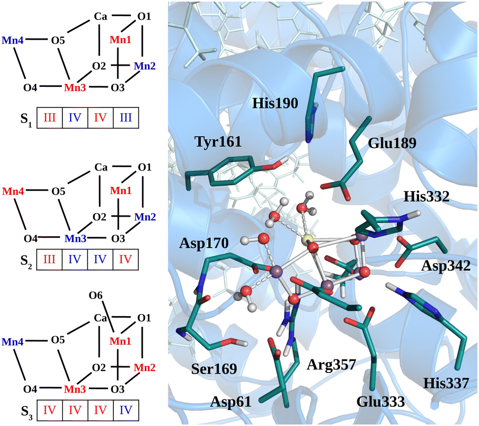
The heavy atom positions chosen as the starting configuration for our calculations are based on the structure from the crystallographic data of the oxygen-evolving photosystem II at 1.9 Å resolution (PDB ID: 3WU221). The dimer has been placed into a DOPC membrane and solvated in TIP3P water. Then, 3 ns of classical MD simulation with harmonic position restraints on the heavy atoms of the protein, cofactors and crystal waters at constant volume and temperature (T = 298 K) were carried out, followed by 3 ns of MD simulation with the same harmonic position restraints in NPT ensemble (T = 298 K and P = 1 bar) as described in our previous work.50 Starting from the last step of the position restrained classical MD trajectory in NPT ensemble, a portion of approximately 40![[thin space (1/6-em)]](https://www.rsc.org/images/entities/char_2009.gif) 000 atoms has been used for the QM/MM calculations, including the Mn4CaO5 cluster, the D1, D2, and CP43 protein domains, as well as the corresponding cofactors, water molecules, and ions. The quantum region treated at DFT level consists of the Mn4CaO5 cluster, the first-sphere ligands (Asp170, Glu189, His332, Glu333, Asp342, Ala344, and CP43-Glu354), the second-sphere residues (Asp61, Tyr161, His190, His337, Ser169, and CP43-Arg357), and the four water molecules directly bound to the metal cluster, consistently with previous calculations (see Fig. 1).8,10,50–55 Additionally, the ten water molecules closest to the cluster and the chloride anion nearby Glu333 are also included in the QM region. The rest of the system is described by the classical force field. The AMBER99SB force field56 was used to describe the topology of the protein residues, while the cofactors present in the structure were described by the general AMBER force field (GAFF),57 as done in ref. 50 and 58. During the QM/MM-MD the positions of the classical Cα atoms have been constrained to the X-ray positions.
000 atoms has been used for the QM/MM calculations, including the Mn4CaO5 cluster, the D1, D2, and CP43 protein domains, as well as the corresponding cofactors, water molecules, and ions. The quantum region treated at DFT level consists of the Mn4CaO5 cluster, the first-sphere ligands (Asp170, Glu189, His332, Glu333, Asp342, Ala344, and CP43-Glu354), the second-sphere residues (Asp61, Tyr161, His190, His337, Ser169, and CP43-Arg357), and the four water molecules directly bound to the metal cluster, consistently with previous calculations (see Fig. 1).8,10,50–55 Additionally, the ten water molecules closest to the cluster and the chloride anion nearby Glu333 are also included in the QM region. The rest of the system is described by the classical force field. The AMBER99SB force field56 was used to describe the topology of the protein residues, while the cofactors present in the structure were described by the general AMBER force field (GAFF),57 as done in ref. 50 and 58. During the QM/MM-MD the positions of the classical Cα atoms have been constrained to the X-ray positions.
 |
| | Fig. 1 Structural sketch of Mn4Ca cluster and the respective spin/redox for each studied state are shown in the left panel. In the right panels are shown the residues included in the QM region for all the QM/MM simulations. | |
For the starting configuration of the QM region in the S1 state we used the optimized geometry in the oxidation and protonation state associated with that state.11 For the S2 state we used the optimized coordinates of the open cubane conformer (named SA2) as in other theoretical studies.28,29 Eventually, the geometry of the S3 state was obtained by optimization after adding an hydroxide, and imposing all the Mn ion as (IV) from the S2 open cubane structure.27,55 All the three QM/MM calculations have been carried out using the CP2K package in a mixed quantum/classical approach as described elsewhere.59 The electrostatic coupling between the classical and the quantum region of the system is treated by means of fast Gaussian expansion of the electrostatic potential.60 The ab initio molecular dynamics simulations have been carried out in NVT ensemble for at least 30 ps, after 3 ps of equilibration, with a time step of 0.5 fs. The system temperature has been stabilized with a thermal bath at 298 K using the Nosé–Hoover algorithm61–63 with a time constant of 0.1 ps. The QM region is contained in a cubic cell of side 28.0 Å, and it is described using the PBE functional with Hubbard correction scheme,64–66 with a value of U = 1.16 eV applied on the Mn ions, which was parameterized for the same system in a previous work.50 We employed a plane-wave expansion cutoff set to 320 Rydberg, using DZVP-MOLOPT-SR-GTH Gaussian basis,67 as described in ref. 50. The ground spin states for the three systems have been chosen consistently with previous computational works28,29,39,55 and with the experimental evidences:27,68S = 0 for S1,  for S2, and
  for S3.
2.2 Vibrational modes analysis
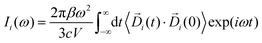
The infrared absorption spectra of the simulated systems have been calculated using the QM/MM ab initio MD trajectories by means of Fourier transformation of the molecular dipole ![[D with combining right harpoon above (vector)]](https://www.rsc.org/images/entities/i_char_0044_20d1.gif) (t) autocorrelation function following previous works:69–73
(t) autocorrelation function following previous works:69–73| |  | (1) |
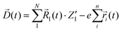
The calculated infrared spectra implicitly include both thermal and anharmonicity effects in a classical fashion. Here, the dipole autocorrelation function can be computed using the dipole moment of the entire QM which is usually provided by any simulation engine. However, this approach does not allow to associate any spectral band with a specific molecular mode. Thus, we chose a different approach for the dipole calculation that also allows to evaluate the dipole fluctuation arising from a specific molecular moiety (i.e. a protein residue or the Mn4Ca cluster). In this framework, the total dipole moment for each frame of the MD trajectories has been obtained from the positions and charges of each particle in the system (both nuclei and electrons). The positions of the nuclei during the trajectory were taken from MD simulations. The charge of each one is defined as the nuclear charge plus the charge of all the core electrons, namely “nuclear valence charge” and reported as  in eqn (2). On the other hand, the positions of the electrons along the trajectory were calculated using the Wannier function center (WFC) method.69,70,74,75 This method allows us to determine the fictitious position of each electron as the highest probability of the maximum localized function of Kohn–Sham orbitals. Also, the sum of the nuclear valence charges
  from all the nuclei and all the WFC is equal to the total charge of the system. Under these conditions, the total dipole moment of throughout the MD trajectory can be calculated as:
| |  | (2) |
In eqn (2), N and ![[R with combining right harpoon above (vector)]](https://www.rsc.org/images/entities/i_char_0052_20d1.gif) I(t) are respectively the total number and positions for all the nuclei. As well, n and
I(t) are respectively the total number and positions for all the nuclei. As well, n and ![[r with combining right harpoon above (vector)]](https://www.rsc.org/images/entities/i_char_0072_20d1.gif) I(t) are the same quantities for the all the electrons, and e is module of the electron charge. As a summation, this dipole can be easily divided in components, allowing for the calculation of their respective dipole auto-correlations. This approach provides a valuable tool for spectral interpretation.69,72,74,76 A divisible dipole allows us to identify very minute contributions (down to a single particle contribution) to the system's total dipole. By applying the eqn (1) to the sub-section dipoles it is possible in principle to calculate the analog of the infrared intensity for a selected moiety:
I(t) are the same quantities for the all the electrons, and e is module of the electron charge. As a summation, this dipole can be easily divided in components, allowing for the calculation of their respective dipole auto-correlations. This approach provides a valuable tool for spectral interpretation.69,72,74,76 A divisible dipole allows us to identify very minute contributions (down to a single particle contribution) to the system's total dipole. By applying the eqn (1) to the sub-section dipoles it is possible in principle to calculate the analog of the infrared intensity for a selected moiety:
| |  | (3) |
In eqn (3), Di (t) the partial dipole is obtained from the sum of the particles of the i-region. This can represent a good alternative to the zero-temperature decomposition method to identify the nature of each spectral feature. However, in the modeling of systems where the electron densities of different regions across a partitioning strongly interact, the sum of all the single Ii(ω) intensities from each dipole components of the system can significantly diverge from the IR spectrum calculated on the dipole of the entire system. This discrepancy arises from neglecting the double counting for sub-dipoles in the auto-correlation scheme. Which can lead to misleading interpretations of the total spectra. To account for such effect when a partitioning of the total dipole is done, the total theoretical formulation has to be written as follows:
| |  | (4) |
here
m is the total number of partitions into which the total system has been divided. If
m = 1, then
eqn (4) is equivalent to
eqn (1). Such a scheme guarantees equality between the calculated total IR intensity
IIR and the sum of all the terms
Ii(
ω) from autocorrelation and

terms from the correlation of each sub-dipole
i-th with the rest of the system. When the subsystems are weakly interacting, thus the correlation term is very small, the
Ii(
ω) spectrum represents the effective infrared absorption of the
i-region; otherwise, the correlation terms between
Di and all the other partition
Dj have to be included. In order to develop an easy-to-use tool capable of processing any small portion of a total dipole without neglecting correlations, we propose a formulation in which the part of the total IR spectra arising from a specific dipole fluctuation is calculated as the Fourier transformation of the dipole correlation between the
i-th dipole (
i(
t)) and the total one (
(0)).
| | 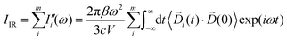 | (5) |
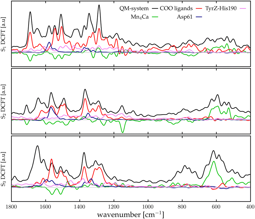
For the sake of brevity, we will refer to the results based on the Fourier transform of the dipole–dipole correlation as “DCFT”'. This formulation has the advantage that the sum of all the  produces exactly the total IR spectra of the entire system. Nevertheless, as it is a quantity obtained from the dipole–dipole correlation, it does not represents anymore an infrared spectrum, but only the mathematical component arising from a specific molecular portion to the total spectrum. In the correlation framework, negative peaks may appear in the DCFT of a specific moiety. This effect is particularly strong in the Mn4Ca DCFT (the green lines in Fig. 2), with several negative peaks in the 1800–1200 cm−1 range. This is due to the fact that the electron density, thus the dipole of such selection, is heavily influenced by the rest of the system, in particular by the COO ligands. Therefore, the negative peaks remove the double counting of the Mn4Ca dipole oscillation due to other part of the system. These negative peaks also indicate where the auto-correlation scheme would struggle to distinguish the contributions from different molecular moieties. In the present study, we selected all the particles belonging to each discussed moiety with a VMD77 script. All the WFC within a certain distance from each nuclei of the selection have been assigned to that moiety. The mandatory requirement is that all the WFC in a selection remain within the same dipole partition throughout the entire simulation. Such result has been obtained with a distance threshold of 1 Å for all the partitioning. For all the analyses, both total spectra calculations and DCFT, the dipoles calculated from eqn (2) have been used. In order to assess the robustness of our data we carried on a convergence test over the timescale of our simulations and found that the total theoretical spectra can be considered as converged after ∼20 ps of simulation. A detailed discussion of the convergence of the spectra is reported in the ESI† (Section 1 and Fig. S1–S5).
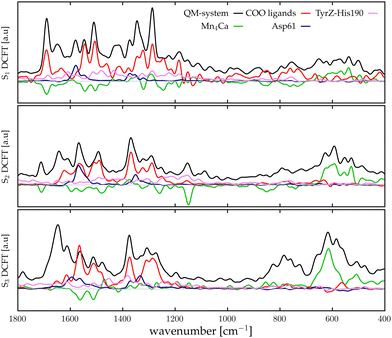 |
| | Fig. 2 Theoretical infrared intensities (black lines) and sub-systems dipole correlation FT of the states S1 (top), S2 (middle), S3 (bottom). The curves colour pattern represents: Mn4Ca cluster (green), first shell COO ligands (red), second shell Asp61 (blue) and second shell TyrZ-His190 couple (pink). The grey line corresponds to the zero value. | |
3 Results and discussion
3.1 Theoretical total spectra
The calculation method of the infrared spectra is based on the Fourier transform of the total dipole autocorrelation function (eqn (1)).69–73 In this way, it is possible to calculate the theoretical IR spectra of the reaction core of the PSII, which is fully included in the QM region using the total dipole of the quantum region. Fig. 2, report by black curves the calculated IR spectra S1, S2, and S3 states. It is important to keep in mind that only these spectra, calculated with FT of the total dipole autocorrelation, can be directly compared with the experimental IR spectra. All the other plots originate from dipole correlation FT (DCFT) of the local dipole fluctuations of a portion of the QM region. Thus, they are only meaningful for the identification of the single vibrational modes. For the sub-system analysis we selected the regions whose experimental assignments have been most discussed in the literature: the Mn4Ca cluster (green lines in Fig. 2), the first shell COO ligands of the cluster all together (red lines in Fig. 2), the second shell ligands Asp61 (blue lines), and eventually, the TyrZ-His190 couple (pink lines). The dipole of such partitions of the system have been calculated as described in the Method section. In the present work, only the Mn4Ca DCFT will be additionally partitioned and discussed in detail. The total spectra, as expected, show the most significant intensities in the region of the symmetric/asymmetric stretching of the COO ligands (i.e., 1200–1800 cm−1 range), and also in the low-frequency region associated with the manganese oxides vibrational modes (i.e., 400–700 cm−1 range). However, this first separation of the total dipole into large portions still leads to a challenging interpretation of the single peaks in both mid and low frequency regions. Further analysis of the Mn4Ca cluster fingerprint region will be discussed in the next sections.
3.2 Theoretical differential spectra
Assuming that the major modifications of the photosynthetic protein along the Kok–Joliot cycle take place in the first and second shell ligands, that have been considered in our model, it can be possible to estimate the differential FTIR spectra between the S-states.35 In Fig. 3, the differential spectra obtained by subtracting the total spectra (black curves reported in Fig. 2) are compared with experimental data from Kimura and coworkers.46 These spectra cover the range between 680 to 400 cm−1, where most of the bands corresponding to the Mn–O vibrational modes of the catalytic cluster can be found. The reported differential spectra refer to the S2-minus-S1 (S2/S1) difference (red curve) and S3-minus-S2 (S3/S2) difference (yellow curve). The agreement is satisfactory, particularly for the S2/S1 spectrum difference, where most of the peaks and trends are well reproduced by the theoretical calculation. In particular, the region around 600 cm−1, which is one of the most discussed, is well reproduced. In the case of the S3/S2 differential spectrum, the computational/experimental agreement is slightly less satisfying. However, we may easily assign the two main positive peaks and the negative one around 600 cm−1. The co-presence of several Mn–O moieties in the complex framework of the Mn4Ca cluster does not allow a direct interpretation of the nature of each peak in the differential spectra only on the basis of the autocorrelation scheme. Therefore, we proceed to analyze in further detail the contributions arising from the single moieties of the cluster in the different S-states by means of an identification approach similar to the one employed in our previous work based on velocity autocorrelation.78
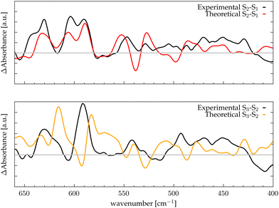 |
| | Fig. 3 Differential spectra obtained with theoretical IR intensities (red and orange lines) compared with the experimental data (black lines) from ref. 46; the grey line corresponds to the zero of the differential spectrum. Top panel: S2-minus-S1; bottom panel: S3-minus-S2. | |
3.3 Mn4Ca cluster fingerprint
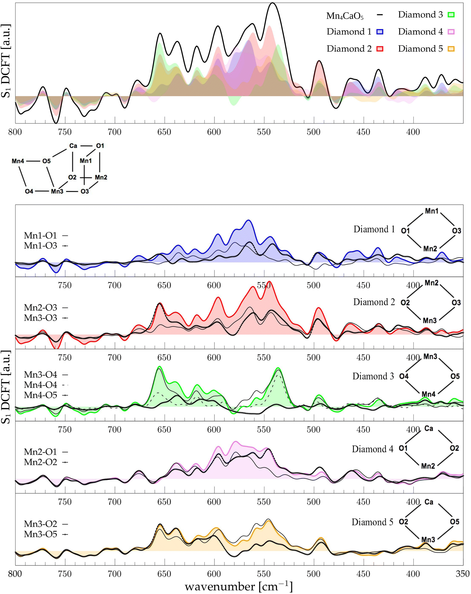
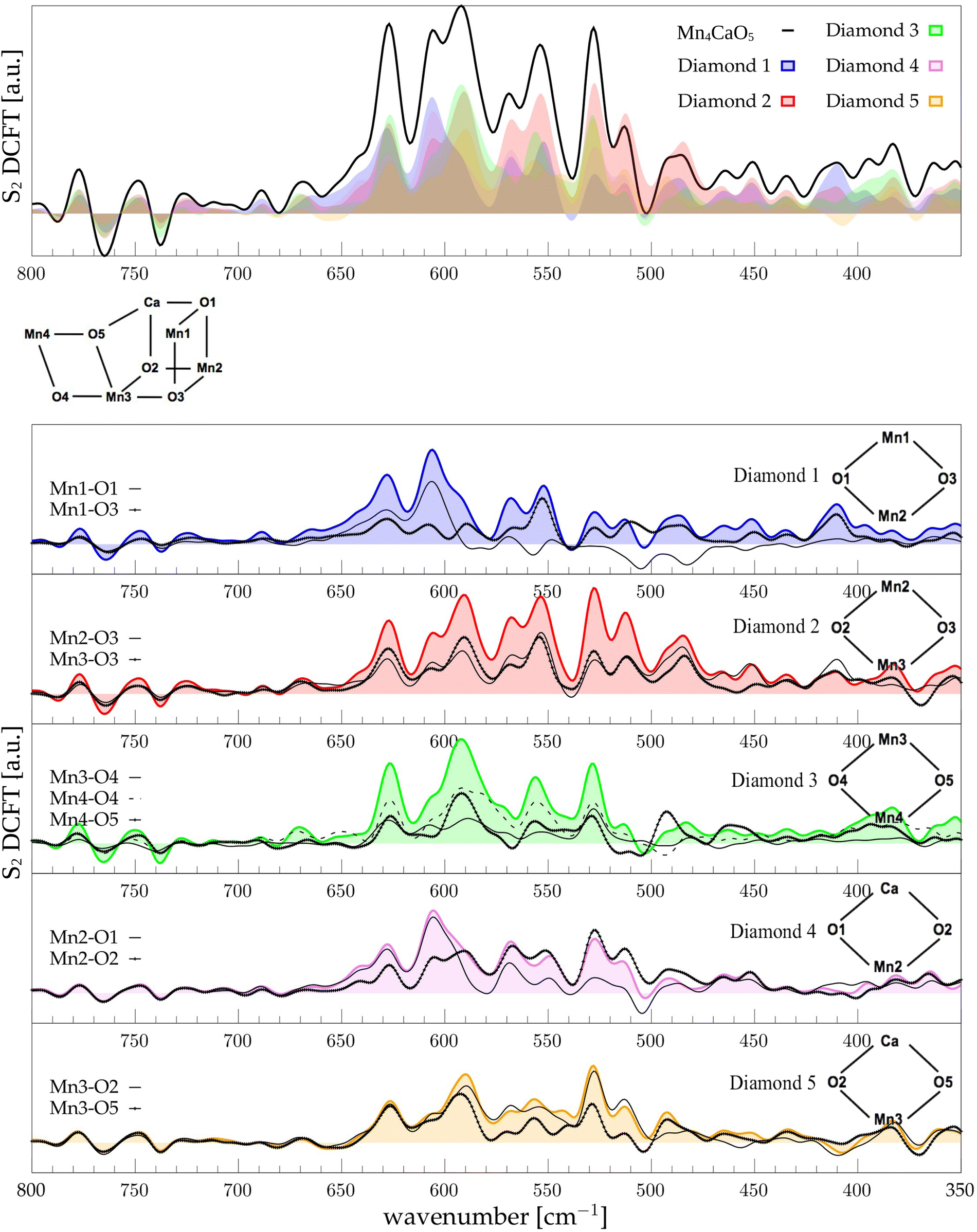
The low-frequency region, which encloses the secret of the catalytic properties of the metal cluster, is one of the most interesting and debated parts of the spectra. In order to assign the vibrational modes arising from the Mn4Ca cluster, the analysis of the dipole correlation FT (DCFT) from the cluster as a whole (green line in Fig. 2) still does not provide enough insights for the experimental comparison. Therefore, a similar approach to effective normal mode analysis (ENMA) as described in our previous work78 has been applied. The procedure consists of dividing the cluster into diamond-like moieties composed of four atoms: two manganese ions and the two μ-oxo bridges connecting them. The ENMA procedure allows for the definition of collective motions from an MD trajectory, which are the analog of the normal modes for zero-temperature calculations. In our case, an empirical approach has been developed to assign each mode to a specific band. Fig. 4–6 show the contributions to the total spectrum of the Mn4Ca cluster modes in each S-state. Additionally, for each state, the contributions of each diamond moiety are reported. To further simplify the assignment, diatomic units composed of one manganese atom and one oxygen atom have been chosen as the fundamental units of the vibrational modes. By choosing two diamonds with a shared side, an adequately intense band that is present in both the DCFT of the two diamonds is identified. As a further confirmation of the band assignment, the value is compared with the spectrum arising solely from the Mn–O couple. In general, all the contributions of the cluster modes can be localized between 650 and 450 cm−1.
 |
| | Fig. 4 The top panel displays the FT of the dipole correlation for the Mn4Ca cluster (black line) and the diamond subunits (colored areas) in the S1 state. In the lower panels, the FT of the dipole correlation for each Mn–O moiety is compared with the same analysis for the diamond in which it is contained. | |
 |
| | Fig. 5 The top panel displays the FT of the dipole correlation for the Mn4Ca cluster (black line) and the diamond subunits (colored areas) in the S2 state. In the lower panels, the FT of the dipole correlation for each Mn–O moiety is compared with the same analysis for the diamond in which it is contained. | |
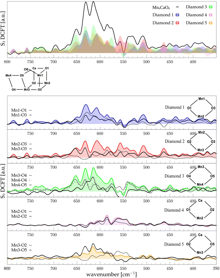 |
| | Fig. 6 The top panel displays the FT of the dipole correlation for the Mn4Ca cluster (black line) and the diamond subunits (colored areas) in the S3 state. In the lower panels, the FT of the dipole correlation for each Mn–O moiety is compared with the same analysis for the diamond in which it is contained. | |
3.4 S1 diamonds DCFT analysis
Starting from the higher frequencies in S1, the DCFT of the Mn4Ca cluster (Fig. 4) shows a double peak between 660 and 640 cm−1. It is present only in the diamonds that include Mn3 and therefore can be straightforwardly assigned to Mn3–O vibrations. Additionally, this peak is particularly intense when also O4 is present, as in D3. Conversely, the 640 cm−1 peak is more intense when Mn3–O5 edge is included. As shown in the bottom panel of Fig. 4, Mn3–O5 modes fills completely the contribution to such a peak in D5 diamond. Similarly, Mn3–O3 DCFT cover for 660 cm−1 peak in D2. Therefore, Mn3–O5 vibration can be assigned to 640 cm−1 and Mn3–O3 vibration to 660 cm−1. 620 cm−1 peak is shared in the majority of the diamonds DCFT, thus representing one of the most diffused mode over the Mn oxide backbone. The peaks at ∼600, 560 and 545 cm−1 are shared between D1, D2 and D4. All of them have Mn2 and two of O1, O2 and O3 oxygen atoms. The strong coupling of such vibrations is not surprising since represents the modes arising from the cubane part of the cluster. Therefore, we assign the peaks at ∼600 cm−1 and 560 cm−1 as Mn1–O2–Mn2 based, and the one at 545 cm−1 as based both on Mn2–O2 and Mn3–O3 modes (see Fig. 4). The peak at 580 cm−1, being shared between D1 and D4, can be assigned to Mn1–O1–Mn2 based modes. This observation suggests a slightly different vibrational frequency for the modes associated with each one of the three Mn vertexes of the cubane (Mn1, Mn2, and Mn3). This behaviour is due to the asymmetrical environment experienced by the three associated oxygen atoms (i.e. O1, O2, and O3). D3 fully accounts the intensity of the band at ∼535 cm−1. Additionally, the DCFT of D3 shows that the major contribution arises from Mn4–O4 (see Fig. 4). Eventually, the 495 cm−1 peak is based on low frequency Mn2 and Mn3 related modes. Approximately, three regions can be identified. The first region, with a high frequency in the range of 650 to 600 cm−1, is associated with highly flexible bridges, such as the Mn3-related modes. The second region, ranging from 600 to 550 cm−1, corresponds to the skeletal modes of the cubane core. Lastly, there is a low-frequency region characterized by highly coupled vibrations and modes originating from the cubane portion of the cluster.
3.5 S2 diamonds DCFT analysis
Following the same scheme used in the previous paragraph, the vibrational modes of the S2 state can also be assigned. In S2, the diamond contributions show more similarities, therefore the vibrational modes are more coupled in this state with respect to S1. This effect can be explained by the increased symmetry of the Mn–Mn and Mn–O distances (as shown in Fig. S6 and S7, ESI†). Particularly, the distribution of Mn4–O5 distances is significantly affected by changes in the oxidation state of the Mn4 ion. The first sharp peak at ∼630 cm−1 arises from Mn3-related modes (Fig. 5), 30 cm−1 red shifted from the S1 position. Also the band at ∼590 cm−1 appears to originate from the same molecular vibrations. Additionally, a significant coupling of these modes with the Mn4–O4 edge can be observed (D3 panel in Fig. 5). Therefore, all of these modes can be associated with highly coupled vibrations arising from D3 and D4 diamonds. It is worth mentioning that the Mn3–O5 DCFT has an intense peak at 590 cm−1 band (see Fig. 5). This significant redshift for the Mn4 related modes can be associated with the sharpening of the Mn–O distance distribution shown in Fig. S7 (ESI†). The 609 cm−1 peak is strongly shared between D1, D2 and D4, and it can be assigned primarily to the Mn2–O1 edge of the cluster. All the four peaks at 570, 555, 525 and 515 cm−1 are present when a part of the diamond D2 is somehow included in the DCFT. Also, a low frequency mode around 485 cm−1 can be assigned to a mixed Mn2–Ox modes.
3.6 S3 diamonds DCFT analysis
In the S3 state no significant variations of the distance distributions with respect to S2 can be observed. Only a small shift to higher distances is observed for Mn1–O3 and Mn3–O3 distributions (see Fig. S7, ESI†). Also, Mn1–Mn4 average distance increases, which is due to the insertion of a new hydroxide group in the Mn1 coordination (Fig. S6, ESI†). Being a dangling ligand, as W1 or W2, the O6–H will not be discussed in the Mn–O motions. As reported in Fig. 1, Mn1 also undergoes oxidation in the S2 to S3 transition. The global effect of the transition is the sharpening of the frequency range, loosing a significant portion of the modes below 600 cm−1 (Fig. 6, top panel). Moreover, all the modes are extremely coupled together if compared with the previous S-states and mainly located between 660 and 550 cm−1. Again, the vibrational mode with highest wavenumber, at 650 cm−1, is a Mn3 related one, mainly shared between D2, D3, and lesser with D5. Using Mn–O moiety dipole correlation FT provided in Fig. 6 we can assign this peak to the vibrational modes of the external and flexible part of the cluster, hence mainly to D3 motions. The band at 630 cm−1 can be observed in all the diamonds DCFT. Notably, the diamonds containing Mn3 and Mn4 have the most intense peak at that specific wavenumber. Conversely, the diamonds containing Mn2 show a broader double peak around the same wavenumber. Thus, we can infer that the molecular vibrations at such energy are widely diffused over most of the cluster. In the peak at ∼615 cm−1 the most relevant DCFT are related to the presence of Mn3 and Mn4, being particularly intense in D3 and D4, where O4 or O5 are also present. Thus, we can assign this band to the modes Mn3–O4–Mn4–O5 face. Also, the band at 630 is more intense when O4 is present, while the one at 615 when O5 is present. We can rationalize this behaviour with the presence of an hydrogen bond between O5 and O6 hydroxide that induce a redshift of the O5 related modes. As mentioned before, the vibrational modes are extremely coupled in this state, indeed, a significant contribution of Mn1 and Mn2 related modes can be found in all the discussed bands. The broad peak around 550 cm−1 can be associated mostly with the Mn2–O2 oscillation (refer to Fig. 6). The other broad peak around 540 cm−1 is mainly originated by the Mn4–O4 moiety with a slight broadening with respect to the same peak in the S2 state. As a general behaviour for S3 we observed that the lower are the frequencies of the modes, the lower are the intensities.
4 Discussion
The final goal of our analysis is to identify spectral contributions of different cluster moieties to unravel the extensive experimental literature concerning vibrational modes, primarily presented as FTIR differential spectra between S-states. In particular in this study focuses on the low-frequencies domain by examining the vibrational modes arising from the Mn4Ca cluster, which is the most discussed in literature due to the catalytic relevance and complexity of interpretation. In the S2-minus-S1 differential spectra firstly reported by Chu et al.44 we notice that the most relevant peaks are between 630 and 560 cm−1. This region is particularly well reproduced by our calculations (Fig. 3, top panel). We have taken into account the peaks at wavenumbers 631(+), 618(−), 606(+), 592(+), and 570(−). The sign of the peaks indicates the peaks origin from S1(−) or S2(+), respectively. Within our interpretation scheme the positive absorption peaks are associated to: (631 cm−1) D2 and D3 coupled modes, (606 cm−1) Mn1–O1–Mn2–O2 mode, and (590 cm−1) Mn3–O4–Mn4–O5 mode. The involvement of O5 into those modes is not surprising. Indeed, several experimental studies provided information that such vibrations are strongly affected by 18O labeling. The negative peak at 618 cm−1 represents a coupling of many cluster modes and cannot be associated with a single mode in the S1 calculated spectrum. The diffuse nature of the vibrational modes across a wide frequency range in S1 is attributed to the significant oscillation of the Mn–O distances compared to the other states (Fig. S7, ESI†), induced by the lower oxidation state of Mn1(III) and Mn4(III). In particular, the wide oscillation of Mn4–O5 towards Mn1 results in a strong coupling of all modes from one side of the cluster to the other. The agreement between the calculated S3-minus-S2 differential spectra and the experimental data is less satisfactory. Nonetheless, we can identify the nature of the two main positive peaks at 628 and 590 cm−1, as well as the small negative ones at 606 cm−1 (see Fig. 3, bottom panel). The wide experimental band between 640 and 610 cm−1 primarily arises from the slight blueshift of the Mn3 and Mn2 related modes, which were resonating at around 600 cm−1 in the previous S1 state (negative peak of the experimental spectra). The most intense positive peak in the spectra at 590 cm−1 can be attributed to a skeletal vibration of the entire cluster. The width of this band in the S3/S2 differential spectrum is notably reduced with respect to the band in the same region in the S2/S1 one. This can be explained by the structural differences observed in the QM/MM-MD simulations, in particular with the increased symmetry of all Mn–O distances.
There are also other reasons for the general discrepancy between calculated frequencies and experiments: first of all, every metastable S-state seems to be composed by a ratio of different states and not only by a single representative structure, though with a large majority of one state.11,23 Moreover, the S3 state is more challenging than the other states to reproduce, since is further from the dark stable state S1 not only in terms of structure (a new water molecule is inserted), but also in terms of resolution and robustness of the proposed X-ray structural comparison.23 The Mn3 related modes are in agreement with isotope labelled FTIR experiment, in which this band is affected by the 18O substitution, suggesting that it is originated by a more flexible Mn–O moiety, likely associated with Mn4 or Mn3.
Furthermore, the presence of a stable moiety like the Mn2–O1 with an increased intensity along the states explains also the presence of the 606/604 cm−1 peak in all the experimental FTIR differential spectra. As a general observation, it would be interesting to see the effect of residue mutation on the low frequency vibrational modes in experiments, since it could make possible to assign specific bands to a specific edge of a vertex of the cluster. Unfortunately, given the intrinsic difficulty of IR techniques in investigating this specific region, very few experimental data are available.
4.1 New theoretical insights from DCFT into Mn4Ca cluster IR interpretation
The results reported here can be considered as a natural evolution of those reported in our previous work based on effective normal mode analysis to the vibrational density of states (VDOS) spectra for the two isomers present in the S2 state.78 However, several technical aspects have been improved. The VDOS is calculated by Fourier transform of the velocity autocorrelation function, thus taking into account also those molecular motions that do not produce a dipole variation, thus IR-inactive. In contrast, the Fourier transform of the dipole autocorrelation tracks all the vibrations that are expected to be IR-active. Additionally, in the present work we add to the simple dipole autocorrelation function a new methodological tool to decipher the origin of the spectral features which is based on dipole fragment correlation function Fourier transform. Eventually, we extended the spectral analysis not only to the S2 state, but also to all the other metastable states of the Kok–Joliot's cycle (i.e. S1 and S3 states). The calculation of the theoretical IR spectra for all the states allowed us to calculate for the first time the PSII reaction center differential spectra in the low frequency region for S2-minus-S1 and S3-minus-S2. Eventually, the MD sampling has been extensively increased, from 10 ps to 30 ps, and such aspect has been shown to be crucial for the spectrum convergence, in particular for the differential spectra. Direct comparison between band assignment using DCFT and VDOS from our previous work is possible only in the S2 state. In this state the band assignment are almost overlapping. In particular, the Mn2 related modes are observed around the 610 cm−1 in both the analysis. The Mn3 related modes and in particular the Mn3–O5, are assigned in the same spectral regions as well. The first around 630/650 cm−1, and the latter at ∼590 cm−1. Also, all the modes at lower wave-numbers are widely coupled all over the cluster in both the modes. Even though the VDOS and DCFT approaches provide very similar results in the band assignment, with the first one it would not be possible to reproduce the differential spectrum.
5 Conclusions
In this computational study, we introduce a novel approach to identify the contributions in the computed infrared spectra obtained by the Fourier transform of dipole correlation function. The strength of this approach lies in the fact that with the correlation method, all non-overlapping partitions are additive, making any decomposition equally valid without affecting the final result. The choice of partitioning is driven solely by the vibrational modes under investigation. Therefore, the iterative decomposition approach reported here, which involves progressively smaller partitions, offers the possibility to discerning the origin of specific infrared bands in strongly interacting systems, such as the Mn4Ca cluster at the core of PSII. The same approach can be easily applied to decipher the spectroscopic features of any other complex systems. The calculated differential IR spectra, reported here for the first time for the low frequency region, are obtained from dipoles calculated on the PSII reaction center simulated with QM/MM molecular dynamics. Such results show good agreement with experimental data, validating the assignments made using the dipole correlation FT (DCFT) approach. Our analysis focuses on the region between 650 to 400 cm−1, where vibrational modes arising from the Mn–O stretching of the metal cluster in the PSII reaction center are observed. We successfully assign most of the differential infrared peaks observed in experimental measurements. Particularly, the region around 600 cm−1 has been extensively discussed over the years, and our theoretical framework enables us to attribute the peaks in this region to a combination of modes involving a mix of Mn2–O and Mn3–O stretching. Additionally, through structural analysis of QM/MM MD simulations, we rationalize the spectral variations associated with transitions between S-states as changes in flexibility of the Mn–O bonds induced by alterations in the redox states of the Mn ions. Furthermore, meticulous analysis based on diamond DCFT suggests that skeletal modes of the cluster are tightly coupled, especially with increasing oxidation states of the Mn ions. Thus, the research of an unambiguous assignment of each experimental band to a single Mn–O bond could be clueless. In conclusion, we introduce and apply a computational strategy that provides a detailed map of vibrational modes along the S1, S2 and S3 of the Kok–Joliot cycle. This approach lays the groundwork for interpreting existing literature and serves as a powerful computational tool for elucidating future spectroscopic experiments.
Author contributions
M. C. and D. N. performed theoretical calculations; M. C. performed data analysis; M. C., G. P., D. N. L. G. contributed to writing – review & editing.
Data availability
All the theoretical spectroscopical data supporting the article have been included in as ESI.†
Conflicts of interest
There are no conflicts to declare.
Acknowledgements
We acknowledge the CINECA computing center under PRACE (project: Pra16-3574) and ISCRA (projects: HP10BT9IR0, HP10C8M10C, HP10CQDXK1) initiatives, and Caliban-HPC centre at the University of L'Aquila for the resources availability and support. Funds were provided by the European Research Council project no. 240624 within the VII Framework Program of the European Union. We acknowledge the use of ChatGPT (https://chat.openai.com/) to identify improvements in the writing style.
Notes and references
- D. G. Nocera, Acc. Chem. Res., 2012, 45, 767–776 CrossRef CAS PubMed.
- J. Barber, Chem. Soc. Rev., 2009, 38, 185–196 RSC.
- C. X. Zhang, C. H. Chen, H. X. Dong, J. R. Shen, H. Dau and J. Q. Zhao, Science, 2015, 348, 690–693 CrossRef CAS PubMed.
- M. Capone, M. Romanelli, D. Castaldo, G. Parolin, A. Bello, G. Gil and M. Vanzan, ACS Phys. Chem. Au, 2024, 202–225 CrossRef CAS PubMed.
- P. Joliot and B. Kok, Bioenerg. Photosxynthesis, 1975, 387–412 CAS.
- P. E. M. Siegbahn, Chem. – Eur. J., 2006, 12, 9217–9227 CrossRef CAS PubMed.
- P. E. M. Siegbahn, Phys. Chem. Chem. Phys., 2012, 14, 4849–4856 RSC.
- M. Capone, D. Narzi and L. Guidoni, Biochemistry, 2021, 60, 2341–2348 CrossRef CAS PubMed.
- M. Capone, A. Sirohiwal, M. Aschi, D. A. Pantazis and I. Daidone, Angew. Chem., 2023, 135, e202216276 CrossRef.
- P. Greife, M. Schönborn, M. Capone, R. Assunção, D. Narzi, L. Guidoni and H. Dau, Nature, 2023, 1–6 Search PubMed.
- D. Narzi, G. Mattioli, D. Bovi and L. Guidoni, Chem. – Eur. J., 2017, 23, 6969–6973 CrossRef CAS PubMed.
- S. Nakamura, M. Capone, D. Narzi and L. Guidoni, Phys. Chem. Chem. Phys., 2019, 22, 273–285 RSC.
- R. J. Debus, M. A. Strickler, L. M. Walker and W. Hillier, Biochemistry, 2005, 44, 1367–1374 CrossRef CAS PubMed.
- A. Boussac, M. Sugiura, A. W. Rutherford and P. Dorlet, J. Am. Chem. Soc., 2009, 131, 5050–5051 CrossRef CAS PubMed.
- M. Askerka, G. W. Brudvig and V. S. Batista, Acc. Chem. Res., 2017, 50, 41–48 CrossRef CAS PubMed.
- N. Schuth, Z. Liang, M. Schonborn, A. Kussicke, R. Assuncao, I. Zaharieva, Y. Zilliges and H. Dau, Biochemistry, 2017, 56, 6240–6256 CrossRef CAS PubMed.
- P. L. Dilbeck, H. Bao, C. L. Neveu and R. L. Burnap, Biochemistry, 2013, 52, 6824–6833 CrossRef CAS PubMed.
- H. Nilsson, F. Rappaport, A. Boussac and J. Messinger, Nat. Commun., 2014, 5, 4305 CrossRef CAS PubMed.
- M. Askerka, D. J. Vinyard, J. Wang, G. W. Brudvig and V. S. Batista, Biochemistry, 2015, 54, 1713–1716 CrossRef CAS PubMed.
- P. Chernev, I. Zaharieva, E. Rossini, A. Galstyan, H. Dau and E.-W. Knapp, J. Phys. Chem. B, 2016, 120, 10899–10922 CrossRef CAS PubMed.
- Y. Umena, K. Kawakami, J.-R. Shen and N. Kamiya, Nature, 2011, 473, 55–60 CrossRef CAS PubMed.
- M. Suga, F. Akita, K. Hirata, G. Ueno, H. Murakami, Y. Nakajima, T. Shimizu, K. Yamashita, M. Yamamoto, H. Ago and J. R. Shen, Nature, 2015, 517, 99–103 CrossRef CAS PubMed.
- J. Kern, R. Chatterjee, I. D. Young, F. D. Fuller, L. Lassalle, M. Ibrahim, S. Gul, T. Fransson, A. S. Brewster and R. Alonso-Mori,
et al.
, Nature, 2018, 563(7731), 421–425 CrossRef CAS PubMed.
- A. Boussac, J.-J. Girerd and A. W. Rutherford, Biochemistry, 1996, 35, 6984–6989 CrossRef CAS PubMed.
- A. Boussac, A. W. Rutherford and M. Sugiura, Biochim. Biophys. Acta, Bioenerg., 2015, 1847, 576–586 CrossRef CAS PubMed.
- T. Lohmiller, V. Krewald, M. P. Navarro, M. Retegan, L. Rapatskiy, M. M. Nowaczyk, A. Boussac, F. Neese, W. Lubitz and D. A. Pantazis,
et al.
, Phys. Chem. Chem. Phys., 2014, 16, 11877–11892 RSC.
- N. Cox, M. Retegan, F. Neese, D. A. Pantazis, A. Boussac and W. Lubitz, Science, 2014, 345, 804–808 CrossRef CAS PubMed.
- D. A. Pantazis, W. Ames, N. Cox, W. Lubitz and F. Neese, Angew. Chem., Int. Ed., 2012, 51, 9935–9940 CrossRef CAS PubMed.
- D. Bovi, D. Narzi and L. Guidoni, Angew. Chem., Int. Ed., 2013, 52, 11744–11749 CrossRef CAS PubMed.
- D. Narzi, D. Bovi and L. Guidoni, Proc. Natl. Acad. Sci. U. S. A., 2014, 111, 8723–8728 CrossRef CAS PubMed.
- H. Isobe, M. Shoji, J.-R. Shen and K. Yamaguchi, Inorg. Chem., 2016, 55, 502–511 CrossRef CAS PubMed.
- Y. Shimada, T. Kitajima-Ihara, R. Nagao and T. Noguchi, J. Phys. Chem. B, 2020, 124, 1470–1480 CrossRef CAS PubMed.
- T. Noguchi and M. Sugiura, Biochemistry, 2003, 42, 6035–6042 CrossRef CAS PubMed.
- T. Noguchi, T. Ono and Y. Inoue, Biochemistry, 1992, 31, 5953–5956 CrossRef CAS PubMed.
- Y. Kato, F. Akita, Y. Nakajima, M. Suga, Y. Umena, J.-R. Shen and T. Noguchi, J. Phys. Chem. Lett., 2018, 9, 2121–2126 CrossRef CAS PubMed.
- M. T. Bernard, G. M. MacDonald, A. P. Nguyen, R. J. Debus and B. A. Barry, J. Biol. Chem., 1995, 270, 1589–1594 CrossRef CAS PubMed.
- T. Kitajima-Ihara, T. Suzuki, S. Nakamura, Y. Shimada, R. Nagao, N. Dohmae and T. Noguchi, Biochim. Biophys. Acta, Bioenerg., 2020, 1861, 148086 CrossRef CAS PubMed.
- R. J. Debus, Biochim. Biophys. Acta, Bioenerg., 2015, 1847, 19–34 CrossRef CAS PubMed.
- M. Capone, D. Narzi, A. Tychengulova and L. Guidoni, Physiol. Plant., 2019, 166, 33–43 CrossRef CAS PubMed.
- S. Nakamura and T. Noguchi, J. Am. Chem. Soc., 2017, 139, 9364–9375 CrossRef CAS PubMed.
- S. Nakamura and T. Noguchi, Proc. Natl. Acad. Sci. U. S. A., 2016, 113, 12727–12732 CrossRef CAS PubMed.
- A. Tychengulova, M. Capone, F. Pitari and L. Guidoni, Chem. – Eur. J., 2019, 25, 13385–13395 CrossRef CAS PubMed.
- C. Berthomieu, R. Hienerwadel, A. Boussac, J. Breton and B. A. Diner, Biochemistry, 1998, 37, 10547–10554 CrossRef CAS PubMed.
- H.-A. Chu, H. Sackett and G. T. Babcock, Biochemistry, 2000, 39, 14371–14376 CrossRef CAS PubMed.
- Y. Kimura and T.-a Ono, Biochemistry, 2001, 40, 14061–14068 CrossRef CAS PubMed.
- Y. Kimura, N. Mizusawa, T. Yamanari, A. Ishii and T.-A. Ono, J. Biol. Chem., 2005, 280, 2078–2083 CrossRef CAS PubMed.
- Y. Kimura, N. Mizusawa, A. Ishii, T. Yamanari and T.-A. Ono, Biochemistry, 2003, 42, 13170–13177 CrossRef CAS PubMed.
- H.-A. Chu, W. Hillier and R. J. Debus, Biochemistry, 2004, 43, 3152–3166 CrossRef CAS PubMed.
- N. Mizusawa, Y. Kimura, A. Ishii, T. Yamanari, S. Nakazawa, H. Teramoto and T.-A. Ono, J. Biol. Chem., 2004, 279, 29622–29627 CrossRef CAS PubMed.
- D. Bovi, D. Narzi and L. Guidoni, New J. Phys., 2014, 16, 015020 CrossRef.
- F. Pitari, D. Bovi, D. Narzi and L. Guidoni, Biochemistry, 2015, 54, 5959–5968 CrossRef CAS PubMed.
- M. Capone, D. Bovi, D. Narzi and L. Guidoni, Biochemistry, 2015, 54, 6439–6442 CrossRef CAS PubMed.
- M. Capone, D. Narzi, D. Bovi and L. Guidoni, J. Phys. Chem. Lett., 2016, 7, 592–596 CrossRef CAS PubMed.
- M. Capone, L. Guidoni and D. Narzi, Chem. Phys. Lett., 2020, 742, 137111 CrossRef CAS.
- D. Narzi, M. Capone, D. Bovi and L. Guidoni, Chem. – Eur. J., 2018, 24, 10820–10828 CrossRef CAS PubMed.
- V. Hornak, R. Abel, A. Okur, B. Strockbine, A. Roitberg and C. Simmerling, Proteins, 2006, 65, 712–725 CrossRef CAS PubMed.
- J. Wang, R. M. Wolf, J. W. Caldwell, P. A. Kollman and D. A. Case, J. Comput. Chem., 2004, 25, 1157–1174 CrossRef CAS PubMed.
- D. Narzi, E. Coccia, M. Manzoli and L. Guidoni, Biophys. Chem., 2017, 229, 93–98 CrossRef CAS PubMed.
- T. Laino, F. Mohamed, A. Laio and M. Parrinello, J. Chem. Theory Comput., 2005, 1, 1176–1184 CrossRef CAS PubMed.
- J. VandeVondele, M. Krack, F. Mohamed, M. Parrinello, T. Chassaing and J. Hutter, Comput. Phys. Commun., 2005, 167, 103–128 CrossRef CAS.
- S. Nosé, J. Chem. Phys., 1984, 81, 511–519 CrossRef.
- S. Nosé, Mol. Phys., 1984, 52, 255–268 CrossRef.
- W. G. Hoover, Phys. Rev. A: At., Mol., Opt. Phys., 1985, 31, 1695–1697 CrossRef PubMed.
- V. I. Anisimov, J. Zaanen and O. K. Andersen, Phys. Rev. B: Condens. Matter Mater. Phys., 1991, 44, 943 CrossRef CAS PubMed.
- S. L. Dudarev, D. N. Manh and A. P. Sutton, Philos. Mag. B, 1997, 75, 613–628 CrossRef CAS.
- S. L. Dudarev, G. A. Botton, S. Y. Savrasov, C. J. Humphreys and A. P. Sutton, Phys. Rev. B: Condens. Matter Mater. Phys., 1998, 57, 1505–1509 CrossRef CAS.
- J. VandeVondele and J. Hutter, J. Chem. Phys., 2007, 127, 114105 CrossRef PubMed.
- A. Boussac and A. W. Rutherford, Biochemistry, 1988, 27, 3476–3483 CrossRef CAS.
- M.-P. Gaigeot and M. Sprik, J. Phys. Chem. B, 2003, 107(38), 10344–10358 CrossRef CAS.
- M.-P. Gaigeot, R. Vuilleumier, M. Sprik and D. Borgis, J. Chem. Theory Comput., 2005, 1, 772–789 CrossRef CAS PubMed.
- M. Thomas, M. Brehm, R. Fligg, P. Vöhringer and B. Kirchner, Phys. Chem. Chem. Phys., 2013, 15, 6608–6622 RSC.
- D. Bovi, A. Mezzetti, R. Vuilleumier, M.-P. Gaigeot, B. Chazallon, R. Spezia and L. Guidoni, Phys. Chem. Chem. Phys., 2011, 13, 20954–20964 RSC.
- M.-P. Gaigeot, Phys. Chem. Chem. Phys., 2010, 12, 3336–3359 RSC.
- N. Marzari and D. Vanderbilt, Phys. Rev. B: Condens. Matter Mater. Phys., 1997, 56, 12847 CrossRef CAS.
- N. Marzari, A. A. Mostofi, J. R. Yates, I. Souza and D. Vanderbilt, Rev. Mod. Phys., 2012, 84, 1419 CrossRef CAS.
- R. Iftimie and M. E. Tuckerman, J. Chem. Phys., 2005, 122, 214508 CrossRef PubMed.
- W. Humphrey, A. Dalke and K. Schulten, J. Mol. Graphics, 1996, 14, 33–38 CrossRef CAS PubMed.
- D. Bovi, M. Capone, D. Narzi and L. Guidoni, Biochim. Biophys. Acta, Bioenerg., 2016, 1857, 1669–1677 CrossRef CAS PubMed.
Footnotes |
| † Electronic supplementary information (ESI) available: Fig. S1 to S4: Convergence of the S1 infrared spectra and some sub-system partitions with increasing simulation timescale. Fig. S5: convergence of S2-minus-S1 differential IR-spectra in the low frequency region. Fig. S6: Mn–Mn distances over the dynamics of the three S-states. Fig. S7: Mn–O distances over the dynamics of the three S-states. See DOI: https://doi.org/10.1039/d4cp01307g |
| ‡ Current affiliation: Center S3, CNR Institute of Nanoscience, Modena, Italy |
|
| This journal is © the Owner Societies 2024 |
Click here to see how this site uses Cookies. View our privacy policy here. 
 Open Access Article
 This Open Access Article is licensed under a Creative Commons Attribution-Non Commercial 3.0 Unported Licence
 *,
Gianluca
Parisse
*,
Gianluca
Parisse
 for S2, and
  for S3.
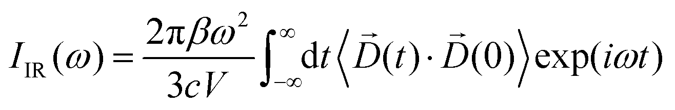
 in eqn (2). On the other hand, the positions of the electrons along the trajectory were calculated using the Wannier function center (WFC) method.69,70,74,75 This method allows us to determine the fictitious position of each electron as the highest probability of the maximum localized function of Kohn–Sham orbitals. Also, the sum of the nuclear valence charges
  from all the nuclei and all the WFC is equal to the total charge of the system. Under these conditions, the total dipole moment of throughout the MD trajectory can be calculated as:
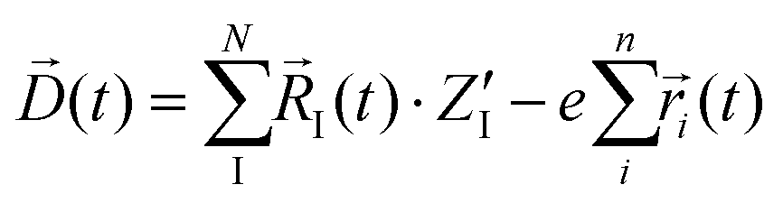


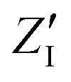
 terms from the correlation of each sub-dipole i-th with the rest of the system. When the subsystems are weakly interacting, thus the correlation term is very small, the Ii(ω) spectrum represents the effective infrared absorption of the i-region; otherwise, the correlation terms between Di and all the other partition Dj have to be included. In order to develop an easy-to-use tool capable of processing any small portion of a total dipole without neglecting correlations, we propose a formulation in which the part of the total IR spectra arising from a specific dipole fluctuation is calculated as the Fourier transformation of the dipole correlation between the i-th dipole (
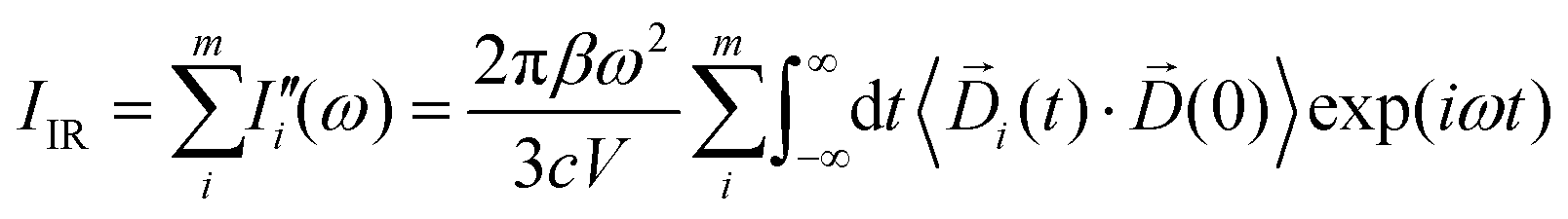
 produces exactly the total IR spectra of the entire system. Nevertheless, as it is a quantity obtained from the dipole–dipole correlation, it does not represents anymore an infrared spectrum, but only the mathematical component arising from a specific molecular portion to the total spectrum. In the correlation framework, negative peaks may appear in the DCFT of a specific moiety. This effect is particularly strong in the Mn4Ca DCFT (the green lines in Fig. 2), with several negative peaks in the 1800–1200 cm−1 range. This is due to the fact that the electron density, thus the dipole of such selection, is heavily influenced by the rest of the system, in particular by the COO ligands. Therefore, the negative peaks remove the double counting of the Mn4Ca dipole oscillation due to other part of the system. These negative peaks also indicate where the auto-correlation scheme would struggle to distinguish the contributions from different molecular moieties. In the present study, we selected all the particles belonging to each discussed moiety with a VMD77 script. All the WFC within a certain distance from each nuclei of the selection have been assigned to that moiety. The mandatory requirement is that all the WFC in a selection remain within the same dipole partition throughout the entire simulation. Such result has been obtained with a distance threshold of 1 Å for all the partitioning. For all the analyses, both total spectra calculations and DCFT, the dipoles calculated from eqn (2) have been used. In order to assess the robustness of our data we carried on a convergence test over the timescale of our simulations and found that the total theoretical spectra can be considered as converged after ∼20 ps of simulation. A detailed discussion of the convergence of the spectra is reported in the ESI† (Section 1 and Fig. S1–S5).