
 Open Access Article
 This Open Access Article is licensed under a Creative Commons Attribution-Non Commercial 3.0 Unported Licence
Tight-binding model predicts exciton energetics and structure for photovoltaic molecules†
Vishal
Jindal
 a,
Mohammed K. R.
Aldahdooh
b,
Enrique D.
Gomez
ac,
Michael J.
Janik
a and
Scott T.
Milner
*ac
a,
Mohammed K. R.
Aldahdooh
b,
Enrique D.
Gomez
ac,
Michael J.
Janik
a and
Scott T.
Milner
*ac
aDepartment of Chemical Engineering, The Pennsylvania State University, USA. E-mail: stm9@psu.edu
bDepartment of Chemistry, The Pennsylvania State University, USA
cDepartment of Materials Science and Engineering, The Pennsylvania State University, University Park, PA 16802, USA
First published on 10th May 2024
Abstract
Conjugated molecules and polymers are being designed as acceptor and donor materials for organic photovoltaic (OPV) cells. OPV performance depends on generation of free charge carriers through dissociation of excitons, which are electron–hole pairs created when a photon is absorbed. Here, we develop a tight-binding model to describe excitons on homo-oligomers, alternating co-oligomers, and a non-fullerene acceptor – IDTBR. We parameterize our model using density functional theory (DFT) energies of neutral, anion, cation, and excited states of constituent moieties. A symmetric molecule like IDTBR has two ends where an exciton can sit; but the product wavefunction approximation for the exciton breaks symmetry. So, we introduce a tight-binding model with full correlation between electron and hole, which allows the exciton to coherently explore both ends of the molecule. Our approach predicts optical singlet excitation energies for oligomers of varying length as well as IDTBR in good agreement with time-dependent DFT and spectroscopic results.
1 Introduction
Organic photovoltaics (OPVs) have emerged as promising alternatives to traditional inorganic solar cells because of their low cost and flexibility.1–3 Active layers of OPVs are blends of electron-donor and electron-acceptor materials, which typically consist of conjugated polymers and/or large conjugated molecules.4–6 Over the past decade, development of conjugated hetero-oligomers known as non-fullerene acceptors, together with polymeric donors, have led to stable and efficient organic photovoltaics with power conversion efficiency in excess of 18 percent.7–10 The tunability of molecular structure and frontier orbital energies of non-fullerene acceptors enables designing novel organic materials for application in high-performing OPV devices.11,12 Detailed structure–property relationships of non-fullerene acceptors as well as the molecular-scale mechanisms contributing to their excellent performance continue to be explored.13,14The conversion efficiency of solar energy to electricity relies on the generation of free charge carriers, which results from the formation and dissociation of excitons.15 Excitons are electrostatically bound electron–hole pairs, formed by electronic transition from the ground state to a singlet excited state upon light absorption.16 The exciton diffuses to the donor–acceptor interface, where electron and hole transfer to the acceptor and donor, respectively, driven by the difference in electron affinity between the two materials. An external electric field facilitates further charge separation into free carriers, which can then be transported to the electrodes. However, failure to dissociate within the exciton lifetime results in the loss of energy collected from photon absorption.17 Thus, understanding and controlling exciton dissociation are crucial for improving the efficiency of organic photovoltaics.18–20
Excitons in organic materials are predominantly formed by excitation of π electrons in conjugated molecules, which may be polymers, small molecules, or oligomers. Because of the low dielectric constant and strong disorder in organic materials, excitons in conjugated molecules are often strongly bound and localized within a single molecule. This leads to long lifetimes and coherent, ultrafast dynamics as a result of their strong interactions with the surrounding molecular environment. Exciton transport occurs by intermolecular hopping via Förster transfer21 and intra-molecular delocalization in extended π-conjugated systems.22 Therefore, accurate modeling of exciton energetics and structure in conjugated molecules is crucial for understanding optoelectronic properties such as charge generation, transport, and recombination, which ultimately enables the design of more efficient OPV devices.23–25
Here, we focus on excitons in large conjugated molecules, such as conjugated oligomers and non-fullerene acceptors. In a molecule, the optical gap corresponds to the energy of the lowest electronic transition to form an exciton, and is measured experimentally by optical absorption. Other “gaps” are also commonly defined. The “fundamental gap” is the difference between the ionization potential and electron affinity of the molecule, which can be determined by gas-phase ultraviolet photoelectron spectroscopy and electron attachment spectroscopy. The “HOMO–LUMO gap” is the energy difference between the highest occupied molecular orbital (HOMO) and lowest unoccupied molecular orbital (LUMO); this theoritical quantity depends on the specifics of the methodology used to calculate the HOMO and LUMO.26 Computationally, the fundamental gap and optical gap have been predicted reliably using various ab initio and semi-empirical methods, including many-body perturbation theory using the GW approximation and the Bethe–Salpeter equations. However, these methods can be computationally intensive, making them less practical for large system sizes and multiple calculations in different configurations.
First-principles calculations using density functional theory (DFT) and time-dependent density functional theory (TD-DFT) are widely used to describe the ground and excited state properties of molecules.27 Although DFT results may depend on the choice of exchange–correlation functional and the amount of Hartree–Fock exchange incorporated, conventional choices can give very good estimates of energy gaps in conjugated molecules. The fundamental gap ΔEfund requires the comparison between the total DFT energy of the N-electron neutral ground state and that of the (N + 1)-electron anion ground state (to determine electron affinity) or that of the (N − 1)-electron cation ground state (to determine ionization potential).26,28 The optical gap ΔEopt is calculated using TD-DFT as the lowest singlet excitation energy, and is generally much lower than the fundamental gap because of the Coulomb attraction between the electron and hole.
The DFT HOMO–LUMO gap ΔEHL determined using exact Kohn–Sham (KS) potential or even density functional approximations such as LDA (local), PBE (semi-local), and B3LYP (hybrid), is reasonably close to the optical gap in molecules:29 it is physically an excitation of the KS system, and not an electron addition as in Hartree–Fock (HF). As noted by Walter Kohn in his Nobel lecture,30,31 the KS potential incorporates the exchange–correlation hole, which means that the KS LUMO is physically different from the Hatree–Fock (HF) LUMO: it does not represent an added electron (as the HF LUMO does), but an excited electron (in the same KS potential as the ground state orbitals), as emphasized by Baerends.32–34 However, use of DFT and TD-DFT can be challenging to use with large system sizes, as well as when modeling the effects of disorder, thermal fluctuations, and the surrounding environment.
Semi-empirical methods, including Pariser–Parr–Pople35 and Su–Schrieffer–Heeger,36 are simple approaches to study electronic structures and excitation in conjugated molecules and polymers. Based on the tight-binding formalism, these methods greatly reduce computational time and allow access to much larger system sizes than DFT calculations. Tight-binding models provide qualitative understanding of excited state static and dynamic properties; quantitative accuracy can also be achieved with careful parametrization. Tight-binding models have also been used to computationally screen optoelectronic properties of various organic small molecules and polymers.37–41 Our group previously used tight-binding model for an infinite chain of poly(3-hexylthiophene) (P3HT) to predict the structure of excitons in bulk and at donor–acceptor interfaces;37,38 to describe polaron formation;38 and to compute polaron hopping barriers and rates.40 Recently, we used local and transferable tight-binding parameters derived from DFT calculations on oligomers and homopolymers of constituent monomers to predict the frontier molecular orbitals of alternating copolymers and non-fullerene acceptors.41,42
Here, we develop a tight-binding approach to describe singlet excitons on conjugated oligomers, using parameters derived from DFT energies of neutral, anion, cation, and excited states of constituent moieties. The aromatic rings that make up a π-conjugated linear molecule are coarse-grained into constituent moieties or “sites”, which is a sensible choice because these rings are structurally rigid and tightly coupled electronically. This coarse-graining reduces the electronic degrees of freedom to only a few local orbitals per site, which greatly reduces computational cost. Molecular disorder is incorporated through flexible dihedral angles between sites. These dihedral angles control the magnitude of hopping terms, which allow for delocalization of charge along the conjugated backbone. Our tight-binding approach represents an exciton as an electron and hole, interacting via the Coulomb potential. To determine the exciton energy and structure, we minimize the total energy with respect to the shape of the electron and hole wavefunctions. Our approach accurately predicts the optical gaps for a diverse set of organic molecules, including oligothiophenes, alternating co-oligomers, and non-fullerene acceptors.
In particular, we apply the tight-binding approach to a heterogeneous conjugated molecule (5Z,5′Z)-5,5′-((7,7′-(4,9-dihydro-s-indaceno [1,2-b:5,6-b′] dithiophene-2,7-diyl)bis (benzo[c][1,2,5] thiadiazole-7,4-diyl))bis(methanylylidene))bis(3-ethyl-2-thioxothiazolidin-4-one) (IDTBR), as a representative non-fullerene acceptor. IDTBR gives high-efficiency organic photovoltaics in combination with poly(3-hexylthiophene) (P3HT) as donor.43 For a symmetric molecule like IDTBR, with two equivalent ends where an exciton can sit, we find that a simple product-wavefunction exciton breaks symmetry. But within our model, we can introduce full correlation between electron and hole, which allows the exciton to coherently explore both ends of the molecule. The resulting optimized two-dimensional exciton wavefunction with full electron–hole correlation can provide qualitative and quantitative descriptions of exciton energetics and structure in large organic molecules.
This paper is organized as follows. We first present a tight-binding model for an electron or a hole on a conjugated molecule, and determine the necessary model parameters from DFT energies for neutral, anion, and cation ground states of the constituent monomers. We then describe contributions to the exciton total energy within our model: the one-body terms that account for onsite and kinetic energy of the electron and hole, and the two-body terms that describe their Coulomb interaction energy. Then we present our results for the optimized singlet exciton on (1) homo-oligomers, (2) alternating co-oligomers, and (3) IDTBR. To validate our approach, predictions for optical gaps are compared to UV-Vis measurements (refer to Fig. S3 in ESI†) and TD-DFT results. Finally, we introduce full correlation between electron and hole, and demonstrate that such correlation is essential for a tight-binding model to represent the singlet exciton on IDTBR.
2 Method
2.1 Tight-binding model
A tight-binding model describes a charge carrier, which could be an electron or a hole, along a conjugated molecule. Electronic degrees of freedom are reduced to only a few local orbitals per site, where an electron or hole occupies sites with an onsite energy, and delocalizes between neighboring sites with hopping matrix elements, with hopping restricted to immediate neighbors.In our work, constituent aromatic moieties are chosen as sites. These moieties are geometrically rigid and tightly coupled electronically, such that their internal electronic structure is only weakly perturbed by the overall chain conformation. For example, IDTBR is modeled as a one-dimensional array of sites, each site corresponding to a monomer unit or moiety along the conjugated backbone – phenylene, thiophene, benzothiadiazole and rhodanine (see Fig. 1).
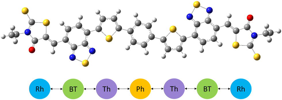 | ||
| Fig. 1 Schematic showing IDTBR molecule's constituent moieties as coarse-grained sites (Ph-phenylene, Th-thiophene, BT-benzothiadiazole, Rh-rhodanine), interconnected to adjacent sites. | ||
The model parameters consist of the onsite energies (ε) for charge carriers to occupy a site, and hopping matrix elements (t) that allow charge carriers to hop from one site to an adjacent site (see Fig. 2). The hopping matrix element t depends on the dihedral angle θ between the two sites, such that t = t0![[thin space (1/6-em)]](https://www.rsc.org/images/entities/char_2009.gif) cos(θ), where t0 is the maximum hopping term in case of a planar geometry.
cos(θ), where t0 is the maximum hopping term in case of a planar geometry.
 | ||
| Fig. 2 A tight-binding model for conjugated molecule represented as an oligomer of length, n. | ||
The Hamiltonian can then be written as follows:
 | (1) |
2.2 Parameters from DFT
We write separate one-body Hamiltonians for the electron and hole on a conjugated oligomer, in which the constituent local hole and electron states are taken as the monomer HOMOs and LUMOs. (More precisely, on each monomer the local hole state is taken as the highest occupied state of the neutral monomer, and the local excited electron state is taken as the highest occupied state of the monomer anion.)For a closed shell molecule in density functional theory, the energy required to add an electron in the LUMO is the difference between the total DFT energy of the N-electron state and the N + 1-electron state, which is the electron affinity (EA) of a molecule. The energy to create a hole, which is equivalent to removing an electron from the HOMO, is the difference between the total DFT energy of the N-electron state and the N − 1-electron state, which is the ionization potential (IP) of the molecule.
Here, we determine the tight-binding model parameters for electrons and holes using formation energies of anions (Ea) and cations (Ec) for constituent monomers and their dimers calculated using DFT. The anion formation energy Ea is the total DFT energy of the (N + 1)-electron state with respect to the N-electron ground state, and the cation formation energy Ec is the total DFT energy of the (N − 1)-electron state with respect to the N-electron ground state:
 | (2) |
The optimized monomer geometry of the N-electron ground state is used to calculate the total DFT energies of N + 1, N and N − 1 electron states of constituent monomers. DFT calculations are performed using a B3LYP hybrid functional with 6-311g(d) basis set using Gaussian 16.
E a and Ec of constituent monomers are the onsite energies εe and εh. To determine the hopping matrix elements te and th between two monomers, we compare Ea and Ec of co-dimers calculated using a 2 × 2 tight-binding Hamiltonian with results of DFT calculation on those co-dimers. For example, Ec for a dimer of monomer 1 and monomer 2 can be calculated using DFT, which we compare to the highest energy eigenvalue of a tight-binding Hamiltonian given by a 2 × 2 matrix:
 | (3) |
On physical grounds, we expect tight-binding parameters to be local; the onsite energy is local to a site, and the hopping matrix element is local to the two adjacent sites. If parameters are local, the values fitted to results for monomers and dimers are transferable to higher oligomers, which greatly simplifies electronic structure calculations for large organic molecules.
 | ||
| Fig. 3 Schematic of optical gap or singlet excitation energy (Ex) in terms of formation energy of anion (Ea) and cation (Ec), and Coulomb interaction energy (Es). | ||
2.3 Singlet exciton energy
An exciton is an electron–hole pair held together by electrostatic interactions. The formation energy Ex of an exciton can be represented as the sum of three terms: the energy Ea to add an electron to the neutral ground state, the energy Ec to add a hole to the ground state, and the stabilization energy Es from the electron–hole attraction:| Ex = Ea + Ec − Es | (4) |
The singlet excitation energy Ex can be calculated using TD-DFT, and the anion and cation energies can be computed using DFT. While DFT calculations are time-consuming and prohibitive for large and disordered systems, DFT and TD-DFT calculations are readily performed for small constituent monomers of organic semiconductors, including thiophene, phenylene, and benzothiadiazole. Using eqn (4) (Fig. 3), we determine the Coulomb interaction energy Es for each moiety. Table 1 lists the formation energy of exciton (Ex), anion (Ea), cation (Ec) and the Coulomb interaction energy parameter (Es) for thiophene, phenylene, benzothiadiazole and rhodanine monomers.
| Monomer | E x | E a | E c | E s |
|---|---|---|---|---|
| Source | TD-DFT | DFT | DFT | eqn (4) |
| Thiophene | 5.684 | 1.514 | 8.889 | 4.717 |
| Phenylene | 6.146 | 1.875 | 9.186 | 4.914 |
| BT | 3.474 | −0.974 | 8.757 | 4.309 |
| Rhodanine | 3.731 | −1.088 | 8.673 | 3.854 |
2.4 Singlet exciton on oligomers
To compute an exciton on an isolated chain of a conjugated molecule, the exciton energy Ex is minimized with respect of the shape of the electron and the hole wavefunctions. We write explicit expressions for Ea, Ec, and Es in terms of electron and hole wavefunctions. The energies Ea and Ec to add an electron or hole in isolation are one-body terms, because they represent the energy of a single charge carrier. The Coulomb energy Es represents the interaction between an electron and a hole, and is therefore a two-body term in the Hamiltonian. | (5) |
 is the wavefunction of the extra electron, and aei is the amplitude of the electronic wavefunction on site i. c†i is the creation operator for an electron acting on the empty LUMO, |0〉. The first term is the onsite energy, and the second term is the hopping energy. εei is the onsite energy of site i, and tei is hopping matrix element for an electron to hop from site i to i + 1.
For a hole, the corresponding energy is:
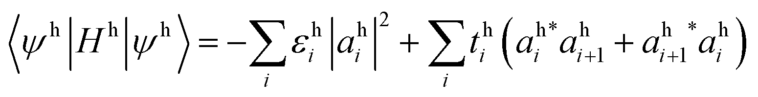 | (6) |
 is the hole wavefunction, where ahi is the amplitude of the hole wavefunction on site i and ci is electron annihilation operator acting on the filled HOMO |V〉.
The one-body term for the hole (eqn (6)) is opposite in sign to the one-body energy term for the electron (eqn (5)), i.e., a hole is the absence of an electron. The sum of electron and hole one-body terms is the energy required to add an electron to the LUMO and remove an electron from the HOMO, in the frozen orbital approximation. Then, the total one-body energy is the LUMO energy minus the HOMO energy, which is, theoretically, the fundamental gap.
| Es = VHLLH − VHLHL | (7) |
In the tight-binding model, the electron and hole wavefunction on a conjugated molecule are written as a linear combination of local LUMO orbitals and HOMO orbitals, respectively, of the constituent monomers on each site. The direct Coulomb energy VHLLH and exchange Coulomb energy VHLHL terms can be divided into onsite (i = j) and offsite (i ≠ j) contributions as follows:
 | (8) |
 | (9) |
Using expression for VHLLH and VHLHL from eqn (8), we can rewrite eqn (7) in terms of direct and exchange Coulomb integrals as:
 | (10) |
For estimating the offsite direct Coulomb integral Dij,38 the HOMO and LUMO located on sites i and j are approximated as Gaussian charge distributions ρ(r):
 | (11) |
 | (12) |
The offsite exchange Coulomb integral Exij can be approximated as the dipole–dipole interaction between transition dipole moments39 located on sites i and j:
 | (13) |
The Coulomb interaction energy (eqn (10)) for a conjugated molecule containing n constituent monomers is rewritten using eqn (12) and (13) as:
 | (14) |
 | (15) |
To calculate the exciton, we minimize the exciton energy E(n)x with respect to the electron (aei) and hole (aei) wavefunction amplitudes, subject to normalization constraints. We neglect the small offsite contributions to the exchange Coulomb energy; onsite exchange is already accounted in the onsite Coulomb interaction parameter. The minimized exciton energy is the predicted singlet excitation energy, and the corresponding onsite amplitudes of the electron and hole wavefunctions are the predicted exciton structure.
Singlet excitation energies for isolated molecules were calculated from TD-DFT using B3LYP/6-311g(d), to compare with model predictions. Exciton energies for some oligomers have also been measured experimentally using UV-Visible absorption spectra. UV-Visible measurements were carried on dilute solutions of molecular compounds to minimize intermolecular interactions; specific experimental details are provided in ESI.† We take the long-wavelength absorption peak from the UV-Vis spectra for each compound given in Fig. S1 (ESI†) to correspond to its singlet excitation energy.
3 Results
3.1 Exciton on homo-oligomers
For a homo-oligomer, the electron and hole onsite energies εe and εh, and the onsite Coulomb interaction parameter Es are the same for every monomer, as are the electron and hole hopping matrix elements te and th between the monomers (Fig. 4). The hopping matrix elements are calculated by comparing the anion/cation energies of homo-dimer (E(2)a/E(2)c) and monomer (E(1)a/E(1)c) as given by: te = E(1)a − E(2)a and th = E(1)c − E(2)c. The smearing length for a monomer was set to σ = Δ/2, where Δ is distance between adjacent monomers. The transition dipole moment μ for a constituent monomer is computed as the integral 〈ψh|r|ψe〉, in which ψh and ψe are the HOMO and LUMO wavefunctions for the monomer, taken from cube files generated by DFT calculations using B3LYP/6-311g(d).The values of monomer parameters are summarized in Table 2. We minimize the exciton energy with respect to onsite amplitudes of electron (aei) and hole (ahi), to predict the optimal exciton on homo-oligomers for varying number of monomers.
 | ||
| Fig. 4 Tight-binding model for homo-oligomer with tight-binding parameters ε and t. | ||
| Monomer | ε e | t e | ε h | t h | E (1)s | Δ | μ |
|---|---|---|---|---|---|---|---|
| Units | eV | eV | eV | eV | eV | Å | ea 0 |
| Thiophene | 1.51 | 1.32 | −8.89 | −1.23 | 4.72 | 4.05 | 1.30 |
| Phenylene | 1.88 | 1.29 | −9.19 | −1.29 | 4.91 | 4.34 | 1.44 |
| Benzothiadiazole | −0.97 | 0.82 | −8.76 | −0.89 | 4.31 | 4.42 | 1.42 |
| Rhodanine | −1.09 | 1.45 | −8.67 | −0.65 | 3.85 | 6.25 | 2.32 |
Fig. 5 compares the predicted singlet excitation energies for oligothiophenes versus chain length to TD-DFT results and experimental UV-Vis measurements. The singlet excitation energy for a thiophene monomer is taken as the HOMO → LUMO transition given by vacuum ultraviolet (VUV) photoabsorption spectrum.44 UV-Visible spectra for oligothiophene with two, three, four and six monomers are given in Fig. S1 of the ESI.† Our tight-binding model accurately predicts the excitation energy for a series of isolated oligothiophenes.
 | ||
| Fig. 5 Optimized singlet excitation energy (orange) compared to TD-DFT results (blue) and UV-Vis measurements (green) for a series of oligothiophenes. | ||
Fig. 6 displays the optimal exciton structure on hexathiophene in all-trans configuration. The electron and hole wavefunctions coincide, localizing the exciton at the molecule center, mainly within the middle four thiophene rings. This tendency for localization applies to excitons in longer oligothiophenes as well, preferring the central four to five rings. In homo-oligomers, no specific site is favored for the electron or hole. Consequently, optimal excitons display unimodal electron and hole wavefunctions, which strongly overlap to minimize the energy by maximizing the Coulomb attraction.
 | ||
| Fig. 6 Optimal exciton on sexithiophene. The hole wavefunction (orange) completely overlaps the electron wavefunction (blue). | ||
We also compute the optimal exciton for a series of phenylene and benzothiadiazole (BT) homo-oligomers. The tight-binding model reasonably predicts the optical gap for both sets of oligomers when compared to TD-DFT results, as depicted in Fig. 7.
 | ||
| Fig. 7 Optimized singlet excitation energy (orange) compared to TD-DFT results (blue) for a series of (a) phenylene and (b) benzothiadiazole homo-oligomers. | ||
3.2 Exciton on alternating co-oligomers
Alternating co-oligomers consist of two different monomers alternating along a conjugated molecule. Using a tight-binding model, a charge carrier along an alternating co-oligomer is represented as a series of sites with two different onsite energies, ε1 and ε2, which correspond to the two types of constituent monomers (Fig. 8). These sites are connected by a hopping matrix element t12, facilitating delocalization between the two co-monomers. To predict an optimal exciton on an alternating co-oligomer of length n, the exciton energy as described in eqn (15), is minimized with respect to electron and hole onsite amplitudes along the oligomer. | ||
| Fig. 8 Tight-binding model for alternating co-oligomer consisting of 6 constituent monomers with onsite parameters, ε1 and ε2, and hopping matrix element, t12. | ||
Onsite parameters are local to a site and can be used without any modifications, as shown in Table 2. This includes the onsite energies and the onsite Coulomb interaction parameter for constituent monomers such as phenylene, thiophene, benzothiadiazole, and rhodanine.
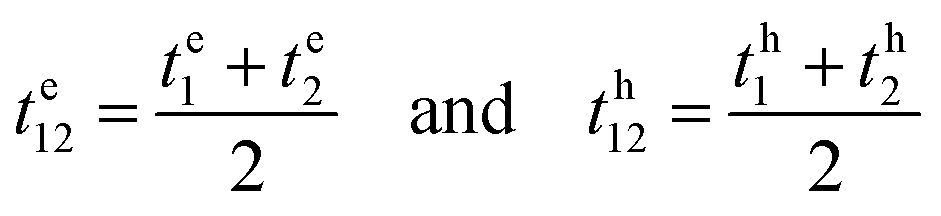
The hopping matrix elements te12 and th12 are calculated by fitting a 2-site tight-binding model for a co-dimer (consisting of monomer 1 and monomer 2) to the formation energy of anion (Ea) and cation (Ec), which are compared to DFT results for the co-dimer. The tight-binding Hamiltonian takes the form of a 2 × 2 matrix with onsite energies ε1 and ε2 as diagonal terms, and t12 as the off-diagonal terms. For both thiophene–phenylene and thiophene–benzothiadiazole dimers, the hopping matrix elements fitted using the dimer tight-binding Hamiltonian turnout to be the same as the average of homo-oligomer hopping matrix elements from Table 2, such that:
 | (16) |
| Co-monomers | t h12 | t e12 | Δ 12 | E x (TD-DFT) | E x (model) |
|---|---|---|---|---|---|
| Thiophene–phenylene | 1.26 | 1.31 | 7.93 | 4.38 | 4.38 |
| Thiophene–benzothiadiazole | 1.06 | 1.07 | 8.00 | 2.60 | 2.62 |
| Benzothiadiazole–rhodanine | 0.56 | 1.04 | 10.09 | 2.56 | 2.64 |
Fig. 9 and 10 compare the singlet excitation energy calculated by our tight-binding model with TD-DFT and experimental results, for varying lengths of alternating thiophene–phenylene and thiophene–benzothiadiazole co-oligomers. Experimental singlet excitation energies are obtained from measured UV-Visible spectra for both thiophene–phenylene and thiophene–benzothiadiazole co-oligomers containing two, three and five monomers, as given in ESI† (Fig. S3).
 | ||
| Fig. 9 Singlet excitation energy for thiophene–phenylene alternating co-oligomers for varying length starting from a single thiophene monomer (labeled as 1 on x-axis), predicted using the tight-binding model (orange) compared to TD-DFT results (blue) and UV-Vis measurements (green). | ||
 | ||
| Fig. 10 Singlet excitation energy for thiophene–benzothiadiazole (BT) alternating co-oligomers for varying length starting from a single thiophene monomer (labeled as 1 on x-axis), predicted using the tight-binding model (orange) compared to TD-DFT results (blue) and UV-Vis measurements (green). | ||
Without adjusting any parameters previously fitted to DFT calculations on individual monomers and co-dimers, the tight-binding model accurately predicts singlet excitation energies for series of thiophene–phenylene alternating co-oligomers compared to both TD-DFT and experimental UV-Vis results.
For a series of thiophene–benzothiadiazole alternating co-oligomers, the tight-binding model predicts singlet excitation energies well compared to TD-DFT, but experimental UV-Vis results are approximately 0.5 eV higher than both model-predicted and TD-DFT excitation energies, as shown in Fig. 10(a). One possible cause of this discrepancy is an inconsistent value of E(1)s parameter for BT, which depends on the singlet excitation energy Ex of BT monomer. Ex of BT monomer from TD-DFT is 3.47 eV, while from experimental results Ex for BT monomer is close to 3.97 eV, as obtained from UV-Visible spectra for BT given in Fig. S3 (ESI†), and near UV spectra for 2,1,3-benzothiadiazole.45
If we use the Ex of BT monomer from experiment instead of TD-DFT to fit the E(1)s parameter for BT, the agreement between tight-binding model and experimental UV-Vis results is improved, as shown in Fig. 10(b).
Fig. 11(a) shows the optimal exciton structure within a thiophene–phenylene (Thio–Ph) alternating co-oligomer comprising six monomers, with electron and hole wavefunctions overlapping each other completely. The exciton prefers to occupy the middle of the thiophene–phenylene hexamer, more generally concentrating at the center of a thiophene–phenylene alternating co-oligomer having a odd number of sites. Note that the exciton leans toward the thiophene end of the molecule because both electron and hole prefer to occupy thiophene compared to phenlyene. This preference results from differences in onsite energies between the thiophene and phenylene moieties: the lower electron onsite energy (εe) and higher hole onsite energy (εh) on thiophene compared to phenylene (outlined in Table 2) favor the exciton to occupy thiophene.
 | ||
| Fig. 11 The electron (orange) and hole (blue) wavefunction for an optimal exciton calculated on two different alternating co-oligomers consisting of six monomeric sites. | ||
Fig. 11(b) displays the wavefunctions for a thiophene–benzothiadiazole (Thio–BT) hexamer. The electron strongly favors the benzothiadiazole (BT) moiety, which is characterized by high electronegativity relative to thiophene, resulting in a lower electron onsite energy (εe) on BT (−1 eV for BT vs. 1.5 eV for thiophene). While the hole displays a less pronounced preference for the thiophene moiety because of subtle differences in hole onsite energies, the slightly higher onsite Coulomb interaction parameter (E(1)s) for thiophene guides the hole towards thiophene. Consequently, an exciton bias towards the BT end of the molecule arises, resulting from the Coulomb interaction of the electron and hole and the strong electronegativity of BT.
For both homo- and co-oligomers, the optimal exciton configuration reflects a balance between the influence of one-body kinetic energy, which tends to spread the carrier wavefunctions across the molecular backbone, and Coulomb interactions that promote the carrier localization.
3.3 Exciton on IDTBR
Our approach can equally well be applied to non-fullerene acceptors, such as IDTBR. This hetero-oligomer is composed of seven constituent moieties (see Fig. 1). At its core, two thiophene rings are bridged to a phenyl ring to form indacenodithiophene. This electron-rich core is flanked on both sides by two electron-withdrawing groups, benzothiadiazole and (3-ethyl)rhodanine. Fig. 12 depicts the tight-binding model for IDTBR, with four different onsite energies (εPh, εBT, εTh, and εRh) and three different hopping matrix elements (tTh–Ph, tTh–BT, and tBT–Rh). | ||
| Fig. 12 Tight-binding model for IDTBR with tight-binding parameters – εPh, εBT, εTh and εRh, and hopping matrix elements – tTh–Ph, tTh–BT and tBT–Rh. | ||
These parameters already computed from the individual monomers and co-dimers are listed in Tables 2 and 3. Table 4 summarizes the tight-binding parameters (εe, εh, te, th), the onsite Coulomb interaction parameter (Es,I), and the characteristic length (σI) for the constituent monomers of IDTBR. We use these parameters without adjustment to compute the IDTBR exciton.
| Monomer (I) | ε e I | ε h I | E s,I | σ I (Å) | Pair (I − J) | t h I−J | t e I−J |
|---|---|---|---|---|---|---|---|
| Phenylene (Ph) | 1.88 | −9.19 | 4.91 | 4.34 | Th–Ph | −1.26 | 1.31 |
| Thiophene (Th) | 1.51 | −8.89 | 4.72 | 4.05 | Th–BT | −1.06 | 1.07 |
| Benzothiadiazole (BT) | −0.97 | −8.76 | 4.31 | 4.42 | BT–Rh | −0.56 | 1.04 |
| Rhodanine (Rh) | −1.09 | −8.67 | 3.85 | 6.25 |
As before, to predict the IDTBR exciton, we minimize the energy by adjusting the shapes of the electron and the hole wavefunctions. Table 5 presents the results, which compare the singlet excitation energy obtained from our tight-binding model versus TD-DFT calculations. The tight-binding model accurately predicts the optical gap, differing by only 0.1 eV from the TD-DFT results.
| Method | Excitation energy (eV) |
|---|---|
| TB model | 1.94 |
| TD-DFT | 1.84 |
| Experiment43 | 1.91 |
The IDTBR molecule exhibits symmetry with respect to its center, and we expect that the exciton will mainly reside on the more electronegative BT and rhodanine moieties located at both ends of the molecule. Fig. 13 displays optimized exciton wavefunctions, where the exciton is predominantly localized at the right end of the molecule. Two degenerate exciton structures were identified, with electron and hole wavefunctions localized at either end. Consequently, the symmetry of the exciton is broken, at least when we assume for simplicity that the electron and hole are uncorrelated, so that a product wavefunction can be used.
 | ||
| Fig. 13 The electron (blue) and hole (orange) wavefunctions for optimal exciton on IDTBR calculated using tight-binding model. | ||
But since the IDTBR molecule is symmetric with respect to its center, we expect the exciton to occupy the more electronegative BT and rhodanine moieties at both ends of the molecule. For this to occur, the electron and hole must be correlated, so they can explore both ends of the molecule while remaining close together. In the next section, we incorporate electron–hole correlations, by introducing a two-dimensional wavefunction that depends on electron and hole positions. Within a tight-binding approach, this is relatively easy to do.
4 Correlated exciton
To introduce correlations between the electron and hole, we represent the exciton wavefunction Ψ as a two-dimensional array of values {aij}, where aij is the exciton amplitude located on site (i,j). For an oligomer of length n, the exciton wavefunction comprises n2 parameters, which is easily manageable numerically. This representation can describe the full range of possible correlations between the electron and the hole.The exciton formation energy can be written in terms of amplitudes aij as:
 | (17) |
 .
.
Table 6 presents the singlet excitation energy for an isolated IDTBR molecule, accounting for correlation effects. This energy is approximately 0.1 eV lower compared to the excitation energy calculated with a product wavefunction, and aligns reasonably well with the TD-DFT and experimental results.
| Method | E x (eV) |
|---|---|
| Experiments43 | 1.91 |
| TD-DFT | 1.84 |
| Uncorrelated | 1.94 |
| Correlated | 1.85 |
Fig. 14 displays the IDTBR exciton as a two-dimensional grid, wherein each grid point corresponds to the amplitude ai,j associated with electron index i and hole index j. With full electron–hole correlations, the exciton now localizes symmetrically at both ends of the molecule. The highest amplitudes are observed at sites (2,2) and (6,6), corresponding to the positions of benzothiadiazole moieties.
 | ||
| Fig. 14 2-D exciton wavefunction on IDTBR. The scale for wavefunction amplitude ai,j is given on the right, while the electron index i is represented on y-axis and hole index j is represented on x-axis. | ||
5 Conclusions
We have developed an electronic model based on the tight-binding approximation to describe singlet excitons in large π-conjugated molecules, including conjugated oligomers and non-fullerene acceptors, which find application in the active layers of organic photovoltaics. While free charge carriers tend to delocalize across electron-rich or electron-withdrawing regions of a conjugated molecule, an optimal exciton structure arises due to the interplay between delocalization (one-body kinetic energy) and attractive interactions (two-body energy) of the electron–hole pair.The tight-binding model greatly reduces the number of electronic degrees of freedom by coarse-graining the conjugated backbone into appropriately sized moieties. These sites are characterized by local parameters, for which we introduce a parameterization scheme that uses DFT and TD-DFT results for the energies of neutral, anion, cation, and excited states of the constituent monomers. This approach simplifies computational complexity while maintaining reasonable accuracy, resulting in transferable tight-binding parameters applicable to heterogeneous systems.
Extending the tight-binding framework to compute optical gaps for conjugated oligomers, we investigated the effect of chain length. By minimizing the exciton energy over electron and hole wavefunction shapes, we accurately predicted singlet excitation energies for various conjugated molecules, observing a diminishing trend in excitation energy with increased monomer units, plateauing around 5–6 units. These predictions aligned well with TD-DFT results and experimental UV-Vis spectroscopy measurements done on dilute solutions.
We also examined the impact of different constituent monomers on exciton structures, we accurately predicted singlet excitation energy for a non-fullerene acceptor, IDTBR. For a symmetric molecule like IDTBR, the product wavefunction exciton structure exhibited a broken symmetry. We then extended our model to a fully two-dimensional exciton wavefunctions, which can describe excitons with electron–hole correlations for conjugated organic molecules.
Our computationally efficient and flexible model can be used to study different molecular architectures, and explore the effect of conformational disorder on exciton energy and structure. We can likewise model charge-transfer excitons at a donor–acceptor interface, by allowing electron and hole to spread over two different molecules. When excitons have charge separation (i.e. electron and hole occupy constituent monomers or molecules), there is charge screening due to the surrounding polarizable medium. Therefore, we do need to include a charge screening term when we model CT excitons, which will be considered in a future publication.
Similarly, free electrons or holes resulting from exciton dissociation can be described by introducing interactions with the surrounding dielectric media to stabilize polarons, the shape of which is obtained by minimizing the sum of the interaction energy with the surrounding media and the kinetic energy of the carrier. Our future work will explore these avenues further, including charge transfer excitons, and polaron hopping barriers and rates in organic photovoltaic materials.
Conflicts of interest
There are no conflicts of interest to declare.Acknowledgements
The authors acknowledge funding provided by the Office of Naval Research (ONR) (grant number N00014-19-1-2453), and the Institute for Computational and Data Sciences (ICDS) at Penn State for providing computational resources. We would also like to acknowledge Dr Dursun Burcu for setting up and conducting initial UV-Visible measurements on oligothiophenes.References
- J. Kong, S. Song, M. Yoo, G. Y. Lee, O. Kwon and J. K. Park, et al., Long-term stable polymer solar cells with significantly reduced burn-in loss, Nat. Commun., 2014, 5(1), 1–8 CrossRef PubMed.
- K. A. Mazzio and C. K. Luscombe, The future of organic photovoltaics, Chem. Soc. Rev., 2015, 44(1), 78–90 RSC.
- L. X. Chen, Organic Solar Cells: Recent Progress and Challenges, ACS Energy Lett., 2019, 4(10), 2537–2539 CrossRef CAS.
- B. Zheng, J. Ni, S. Li, Y. Yue, J. Wang and J. Zhang, et al., Conjugated Mesopolymer Achieving 15% Efficiency Single-Junction Organic Solar Cells, Adv. Sci., 2022, 9(8), 2105430 CrossRef CAS PubMed.
- T. Xia, Y. Cai, H. Fu and Y. Sun, Optimal bulk-heterojunction morphology enabled by fibril network strategy for high-performance organic solar cells, Sci. China: Chem., 2019, 62(6), 662–668 CrossRef CAS.
- C. Xu, Z. Zhao, K. Yang, L. Niu, X. Ma and Z. Zhou, et al., Recent progress in all-small-molecule organic photovoltaics, J. Mater. Chem. A, 2022, 10(12), 6291–6329 RSC.
- C. Yan, S. Barlow, Z. Wang, H. Yan, A. K. Y. Jen and S. R. Marder, et al., Non-fullerene acceptors for organic solar cells, Nat. Rev. Mater., 2018, 3, 18003 CrossRef CAS.
- S. Bao, H. Yang, H. Fan, J. Zhang, Z. Wei and C. Cui, et al., Volatilizable Solid Additive-Assisted Treatment Enables Organic Solar Cells with Efficiency over 18.8% and Fill Factor Exceeding 80%, Adv. Mater., 2021, 33(48), 2105301 CrossRef CAS PubMed.
- Y. Wang, J. Lee, X. Hou, C. Labanti, J. Yan and E. Mazzolini, et al., Recent Progress and Challenges toward Highly Stable Nonfullerene Acceptor-Based Organic Solar Cells, Adv. Energy Mater., 2021, 11(5), 2003002 CrossRef CAS.
- L. Zhu, M. Zhang, J. Xu, C. Li, J. Yan and G. Zhou, et al., Single-junction organic solar cells with over 19% efficiency enabled by a refined double-fibril network morphology, Nat. Mater., 2022, 21(6), 656–663 CrossRef CAS PubMed.
- A. Kuzmich, D. Padula, H. Ma and A. Troisi, Trends in the electronic and geometric structure of non-fullerene based acceptors for organic solar cells, Energy Environ. Sci., 2017, 10(2), 395–401 RSC.
- J. A. Schmidt, J. A. Weatherby, I. J. Sugden, A. Santana-Bonilla, F. Salerno and M. J. Fuchter, et al., Computational Screening of Chiral Organic Semiconductors: Exploring Side-Group Functionalization and Assembly to Optimize Charge Transport, Cryst. Growth Des., 2021, 21(9), 5036–5049 CrossRef CAS.
- S. Giannini, W. T. Peng, L. Cupellini, D. Padula, A. Carof and J. Blumberger, Exciton transport in molecular organic semiconductors boosted by transient quantum delocalization, Nat. Commun., 2022, 13(1), 1–13 Search PubMed.
- F. Eisner and J. Nelson, Barrierless charge generation at non-fullerene organic heterojunctions comes at a cost, Joule, 2021, 5(6), 1319–1322 CrossRef.
- R. Ghosh and F. C. Spano, Excitons and Polarons in Organic Materials, Acc. Chem. Res., 2020, 53(10), 2201–2211 CrossRef CAS PubMed.
- G. Tirimbò and B. Baumeier, Ab initio modeling of excitons: from perfect crystals to biomaterials, Adv. Phys.: X, 2021, 6(1), 1912638 Search PubMed.
- A. J. Barker, K. Chen and J. M. Hodgkiss, Distance distributions of photogenerated charge pairs in organic photovoltaic cells, J. Am. Chem. Soc., 2014, 136(34), 12018–12026 CrossRef CAS PubMed.
- W. T. Peng, D. Brey, S. Giannini, D. Dell'Angelo, I. Burghardt and J. Blumberger, Exciton Dissociation in a Model Organic Interface: Excitonic State-Based Surface Hopping versus Multiconfigurational Time-Dependent Hartree, J. Phys. Chem. Lett., 2022, 13(31), 7105–7112 CrossRef CAS PubMed.
- H. Ma and A. Troisi, Modulating the exciton dissociation rate by up to more than two orders of magnitude by controlling the alignment of LUMO+1 in organic photovoltaics, J. Phys. Chem. C, 2014, 118(47), 27272–27280 CrossRef CAS.
- L. Kronik and J. B. Neaton, Excited-State Properties of Molecular Solids from First Principles, Annu. Rev. Phys. Chem., 2016, 67(1), 587–616 CrossRef CAS PubMed.
- K. Feron, W. J. Belcher, C. J. Fell and P. C. Dastoor, Organic solar cells: Understanding the role of forster resonance energy transfer, Int. J. Mol. Sci., 2012, 13(12), 17019–17047 CrossRef CAS PubMed.
- G. Zhang, X. K. Chen, J. Xiao, P. C. Y. Chow, M. Ren and G. Kupgan, et al., Delocalization of exciton and electron wavefunction in non-fullerene acceptor molecules enables efficient organic solar cells, Nat. Commun., 2020, 11(1), 1–10 CrossRef PubMed.
- U. Lemmer, Exciton dynamics in conjugated polymer devices, Conference on Quantum Electronics and Laser Science (QELS) - Technical Digest Series, 1997, 12, 16.
- A. M. Kay, O. J. Sandberg, N. Zarrabi, W. Li, S. Zeiske and C. Kaiser, et al., Quantifying the Excitonic Static Disorder in Organic Semiconductors, Adv. Funct. Mater., 2022, 32(32), 2113181 CrossRef CAS.
- Y. Yao, Establishing a microscopic model for nonfullerene organic solar cells: Self-accumulation effect of charges, J. Chem. Phys., 2018, 149(19), 194902 CrossRef PubMed.
- J. L. Bredas, Mind the gap!, Mater. Horiz., 2014, 1(1), 17–19 RSC.
- S. Huang, Q. Zhang, Y. Shiota, T. Nakagawa, K. Kuwabara and K. Yoshizawa, et al., Computational prediction for singlet- and triplet-transition energies of charge-transfer compounds, J. Chem. Theory Comput., 2013, 9(9), 3872–3877 CrossRef CAS PubMed.
- E. San-Fabián, E. Louis, M. A. Díaz-García, G. Chiappe and J. A. Vergés, Transport and optical gaps in amorphous organic molecular materials, Molecules, 2019, 24(3), 1–16 CrossRef PubMed.
- Y. Shu and D. G. Truhlar, Relationships between Orbital Energies, Optical and Fundamental Gaps, and Exciton Shifts in Approximate Density Functional Theory and Quasiparticle Theory, J. Chem. Theory Comput., 2020, 16(7), 4337–4350 CrossRef CAS PubMed.
- W. Kohn, Nobel Lecture - Electronic Structure of Matter – Wave Functions and Density Functionals, 1999. Available from: https://www.nobelprize.org/prizes/chemistry/1998/kohn/lecture/ Search PubMed.
- W. Kohn, Density functional and density matrix method scaling linearly with the number of atoms, Phys. Rev. Lett., 1996, 76(17), 3168–3171 CrossRef CAS PubMed.
- M. Amati, S. Stoia and E. J. Baerends, The Electron Affinity as the Highest Occupied Anion Orbital Energy with a Sufficiently Accurate Approximation of the Exact Kohn-Sham Potential, J. Chem. Theory Comput., 2020, 16(1), 443–452 CrossRef CAS PubMed.
- E. J. Baerends, Density functional approximations for orbital energies and total energies of molecules and solids, J. Chem. Phys., 2018, 149(5), 054105 CrossRef PubMed.
- E. J. Baerends, O. V. Gritsenko and R. Van Meer, The Kohn-Sham gap, the fundamental gap and the optical gap: The physical meaning of occupied and virtual Kohn-Sham orbital energies, Phys. Chem. Chem. Phys., 2013, 15(39), 16408–16425 RSC.
- K. Jug, Theoretical basis and design of the PPP model Hamiltonian, Int. J. Quantum Chem., 1990, 37(4), 403–414 CrossRef CAS.
- The Su–Schrieffer–Heeger (SSH) model, Lecture Notes in Physics, 2016, 919, 1–22.
- J. H. Bombile, M. J. Janik and S. T. Milner, Tight binding model of conformational disorder effects on the optical absorption spectrum of polythiophenes, Phys. Chem. Chem. Phys., 2016, 18(18), 12521–12533 RSC.
- J. H. Bombile, M. J. Janik and S. T. Milner, Polaron formation mechanisms in conjugated polymers, Phys. Chem. Chem. Phys., 2017, 20(1), 317–331 RSC.
- J. H. Bombile, M. J. Janik and S. T. Milner, Energetics of exciton binding and dissociation in polythiophenes: A tight binding approach, Phys. Chem. Chem. Phys., 2019, 21(22), 11999–12011 RSC.
- J. H. Bombile, S. Shetty, M. J. Janik and S. T. Milner, Polaron hopping barriers and rates in semiconducting polymers, Phys. Chem. Chem. Phys., 2020, 22(7), 4032–4042 RSC.
- P. Tipirneni, V. Jindal, M. J. Janik and S. T. Milner, Tight binding models accurately predict band structures for copolymer semiconductors, Phys. Chem. Chem. Phys., 2020, 22(35), 19659–19671 RSC.
- V. Jindal, M. J. Janik and S. T. Milner, Tight-binding model describes frontier orbitals of non-fullerene acceptors, Mol. Syst. Des. Eng., 2024, 9, 382–398 RSC.
- S. Holliday, R. S. Ashraf, A. Wadsworth, D. Baran, S. A. Yousaf and C. B. Nielsen, et al., High-efficiency and air-stable P3HT-based polymer solar cells with a new non-fullerene acceptor, Nat. Commun., 2016, 7, 11585 CrossRef CAS PubMed.
- D. B. Jones, M. Mendes, P. Limão-Vieira, F. Ferreira Da Silva, N. C. Jones and S. V. Hoffmann, et al., Electronic structure and VUV photoabsorption measurements of thiophene, J. Chem. Phys., 2019, 150(6), 064303 CrossRef CAS PubMed.
- R. D. Gordon and R. F. Yang, The near ultraviolet spectra of 2,1,3-benzothiadiazole and its deuterated and substituted derivatives, J. Mol. Spectrosc., 1971, 39(2), 295–320 CrossRef CAS.
Footnote |
| † Electronic supplementary information (ESI) available. See DOI: https://doi.org/10.1039/d4cp00554f |
| This journal is © the Owner Societies 2024 |