
 Open Access Article
 This Open Access Article is licensed under a
 Creative Commons Attribution 3.0 Unported Licence
Extraction of local structure differences in silica based on unsupervised learning†
Anh Khoa Augustin
Lu
 *ab,
Jianbo
Lin
c,
Yasunori
Futamura
def,
Tetsuya
Sakurai
def,
Ryo
Tamura
*cg and
Tsuyoshi
Miyazaki
*afh
*ab,
Jianbo
Lin
c,
Yasunori
Futamura
def,
Tetsuya
Sakurai
def,
Ryo
Tamura
*cg and
Tsuyoshi
Miyazaki
*afh
aResearch Center for Materials Nanoarchitectonics, National Institute for Materials Science, Tsukuba 305-8568, Japan. E-mail: LU.Augustin@nims.go.jp; augustinlu@gmail.com; TAMURA.Ryo@nims.go.jp; MIYAZAKI.Tsuyoshi@nims.go.jp
bMathematics for Advances Materials Open Innovation Laboratory, National Institute of Advanced Industrial Science and Technology, Sendai 980–8577, Japan
cCenter for Basic Research on Materials, National Institute for Materials Science, Tsukuba 305-0047, Japan
dDepartment of Computer Science, University of Tsukuba, Tsukuba 305-8573, Japan
eCenter for Artificial Intelligence, University of Tsukuba, Tsukuba 305-8573, Japan
fMaster's/Doctoral Program in Life Science Innovation, University of Tsukuba, Tsukuba 305-8577, Japan
gGraduate School of Frontier Sciences, The University of Tokyo, Chiba 277-8568, Japan
hGraduate School of Engineering, Nagoya university, Nagoya 464-8603, Japan
First published on 28th March 2024
Abstract
Silica exhibits a rich phase diagram with numerous stable structures existing at different temperature and pressure conditions, including its glassy form. In large-scale atomistic simulations, due to the small energy difference, several phases may coexist. While, in terms of long-range order, there are clear differences between these phases, their short- or medium-range structural properties are similar for many phases, thus making it difficult to detect the structural differences. In this study, a methodology based on unsupervised learning is proposed to detect the differences in local structures between eight phases of silica, using atomic models prepared by molecular dynamics (MD) simulations. A combination of two-step locality preserving projections (TS-LPP) and locally averaged atomic fingerprints (LAAF) descriptor was employed to find a low-dimensional space in which the differences among all the phases can be detected. From the distance between each structure in the found low-dimensional space, the similarity between the structures can be discussed and subtle local changes in the structures can be detected. Using the obtained low-dimensional space, the β-α transition in quartz at a low temperature was analyzed, as well as the structural evolution during the melt-quench process starting from α-quartz. The proper differentiation and ease of visualization make the present methodology promising for improving the analysis of the structure and properties of glasses, where subtle differences in structure appear due to differences in the temperature and pressure conditions at which they were synthesized.
1 Introduction
Silica (SiO2) is one of the most abundant materials on earth as the major constituent of sand and is an important ingredient for a wide range of applications, such as concrete (with silica fume1), photonics2 or as a gate dielectric in metal–oxide–semiconductors field effect transistors.3 It is the simplest of the silicates and yet it is one of the most technologically relevant.4 Several crystalline forms exist at different pressure and temperature conditions (quartz, coesite, stishovite, cristobalite, tridymite, etc.) as well as in glass form.5–11 For most phases, Si atoms are four-coordinated and form tetrahedra with the surrounding O atoms. However, high-pressure phases such as stishovite and seifertite have six-coordinated Si atoms. Therefore, the external conditions under which the process to synthesize a silica sample is conducted, has an enormous impact on its atomic structure and therefore are strongly related to their properties. Understanding the structural changes is thus a necessity in order to engineer new materials with enhanced properties. Moreover, for disordered materials such as silica glass, the structural differences are subtle and may be localized in a relatively small region, yet exceeding the first-neighbor shell.In recent times, the progress in atomistic simulations has enabled studies of the dynamics of a system with first-principles accuracy.12,13 In order to properly analyze the structural properties, defining quantities of interest is of utmost importance.14–17 Over the last decades, several descriptors have been developed in order to describe local structures, such as the smooth overlap of atomic positions (SOAP).18 Ring statistics based on graph theory was also proposed to study the connectivity of amorphous materials.19–21 The topological features and patterns in materials were also studied by persistent homology.22,23 However, a method that can properly capture the structural differences between phases of silica is still lacking. Most methods rely on averaged quantities and statistics, such as the structure factor or radial distribution functions.24–26 Extracting local information therefore remains a challenging task, exacerbated by the fact that subtle changes may occur locally in a given region. Other methods based on local structures, such as common-neighbor analysis (CNA)27,28 and various functions29,30 have been developed. However, only relatively simple phases such as face-centered cubic (FCC), body-centered cubic (BCC) or hexagonal closed-packed (HCP) could be recognized. For silica and its numerous complex phases, these methods would be unable to distinguish relevant complex phases.
As an alternative method of structural analysis focusing on local structures, an unsupervised learning method combining the two-step locality preserving projections (TS-LPP) method and locally-averaged atomic fingerprints (LAAF) has been recently developed.31 Using this technique, it has been shown that liquid, crystalline, and amorphous structures could be clearly distinguished in Si and SiGe systems. To obtain these results, higher dimensional descriptors focusing on local structures were projected to a two-dimensional space via dimensionality reduction using TS-LPP to facilitate understanding of the local structures. In particular, it is generally difficult to distinguish liquid and amorphous structures only from their local structures, and conventional dimensionality reduction techniques are inadequate for addressing this problem.31 However, when conducting structural analysis of the numerous complex phases of silica, it would be impossible to find a two-dimensional space in which all phases can be distinguished even with TS-LPP.
In this study, we perform a structural analysis for eight structures in silica using the potential of the unsupervised learning method with TS-LPP and LAAF descriptor based on atom-centered symmetry functions (ACSF). The targeted structures are α-quartz, β-quartz, coesite, β-tridymite, β-cristobalite, stishovite, liquid, and glass. It was found that finding a model that distinguishes all phases in a two-dimensional space was unattainable. On the other hand, a four-dimensional space in which all of these phases are separated could be created. From the locations of each phase in the low-dimensional space, the similarity or differences between different phases can be understood. Using this low-dimensional space, the structural evolution from β-quartz to α-quartz at low temperature was followed, and the melt-quench process was analyzed, showing that local changes can be detected by our methodology.
The methodology developed for this study is has the potential to unlock new prospects for elucidating the nature of amorphous materials in future investigations of disordered materials where impurities and interfaces are present, such as in Si/SiO2 interfaces. For such systems, our methodology should be able to detect the subtle variations in local structures that may lead to previously unknown types of structures.
2 Methods
2.1 Structural analysis based on unsupervised learning
An overview of the methodology used for this study to perform structural analysis is depicted in Fig. 1. Atomic configurations of the different phases were generated by molecular dynamics (MD) simulations. From these models, locally averaged atomic fingerprints (LAAF) based on the G2 atom-centered symmetry functions (ACSF) were calculated.32 As discussed by Tamura et al.,31 LAAF are expected to express two different types of locality in the coordination environment around each atom by two cutoffs, Rd and Ra. The first cutoff is used for the definition of ACSF showing the chemical or coordination environments, while the second one is related to the similarity of the chemical environment with the surrounding atoms. The definition of the LAAF descriptor can be found in Appendix A. These descriptors, after feature selection by variance threshold and standardization, were transformed onto a low-dimensional space using the two-step locality preserving projections method (TS-LPP).31 The TS-LPP method consists in using LPP twice, with a reduction from the LAAF dimensionality M (after feature selection) to the intermediate dimension dm and from dm to the target low-dimension dτ. The details of LPP method are explained in Appendix B. In TS-LPP, two hyperparameters (dm and σ) need to be defined. To determine appropriate values for these hyperparameters, the Calinsky–Harabasz score (pseudo-F33) was used for the k-means clustering results in the found low-dimensional space by TS-LPP. A grid exploration was performed to determine the most appropriate values for dm and σ. The same value for σ was used for both LPP steps in the present implementation of the TS-LPP method. Finally, clustering methods (such as k-means clustering or DBSCAN) were used to identify different groups of local structures in the reduced space. | ||
| Fig. 1 Overview of the methodology used for the analysis of silica phases. | ||
2.2 First-principles molecular dynamics
To generate the target atomic configurations, first-principle molecular dynamics (FPMD) simulations were performed using the CONQUEST code.34–36 The Perdew–Burke–Ernzerhof (PBE)37 exchange–correlation functional was used with pseudopotentials.38,39Γ -only calculations were performed with the double-zeta polarized (DZP) basis sets.40 The energy cutoff for the charge density was set to 200 Ha. The temperature was controlled using Nosé–Hoover chains41 and the pressure was controlled by a Parrinello–Rahman barostat.42 The atomic configurations typically contain around 200 to 400 atoms. The time step is 1 fs and simulations of 5000 time steps (5 ps) were performed for each configuration. For the crystalline phases, it was observed that the average positions during constant-volume (NVT) simulations were very close to their initial positions (within 0.2 Å). This suggests that the original crystalline phases are preserved during NVT simulations even at 300 K and 600 K, despite the fact that some of them are stable only at higher temperatures in experiments. Note that we observed some phase transitions in constant-pressure (NPT) simulations, for example the transition from β-quartz to α-quartz structures. While this is of physical relevance, such changes are undesired in this work where the aim is to generate trajectories representative of each phase. Therefore, only NVT trajectories for crystal phases are included in the training set, as reported in Table 1. The change of local structures in the β-to-α quartz transition is analyzed in Subsection 3.4. On the other hand, the trajectories for the liquid and glass phases were generated using the NPT ensemble.| Phase | Si atoms/cell | Conditions | Number of data points |
|---|---|---|---|
| α-quartz | 108 | 300 K (NVT) and 600 K (NVT) | 1080 |
| β-quartz | 108 | 300 K (NVT) and 600 K (NVT) | 1080 |
| β-cristobalite | 64 | 300 K (NVT) and 600 K (NVT) | 640 |
| β-tridymite | 128 | 300 K (NVT) and 600 K (NVT) | 1280 |
| Coesite | 64 | 300 K (NVT) and 600 K (NVT) | 640 |
| Stishovite | 90 | 300 K (NVT) and 600 K (NVT) | 900 |
| Liquid | 108 | 3000 K (NPT) and 4000 K (NPT) | 1080 |
| Glass | 108 | 300 K (NPT) (cooling rate of 1010–13 K s−1) | 2160 |
2.3 Classical molecular dynamics
To generate the initial atomic configurations of liquid and glass phases for FPMD, classical molecular dynamics simulations were performed using the Large-scale Atomic Molecular Massively Parallel Simulator (LAMMPS) software package with GPU acceleration43,44 to generate liquid and glassy structures of SiO2. Munetoh potentials (Tersoff-type) were used to describe the inter-atomic interactions.45 The temperature and pressure were controlled using Nosé–Hoover style non-Hamiltonian equations of motions.46,47 These structures were used as initial configurations for FPMD simulations. The time step was set to 1 fs. From an initial α-quartz crystal, the system was first melted at 5000 K, then cooled down to 300 K with a cooling rate ranging from 1010 K s−1 to 1013 K s−1, resulting in simulation times ranging from to 0.5 ns to 370 ns. Liquid structures were relaxed for 50 ps. These structures were used as initial states for FPMD simulations.3 Structural analysis of silica systems
3.1 Target structures in silica
The detailed composition of the training set is provided in Table 1. The target data set for the structural analysis for silica systems includes eight different phases: α-quartz (stable at room temperature) and β-quartz (high temperature), β-cristobalite (high temperature), β-tridymite (high temperature), coesite (high pressure), stishovite (high pressure), liquid and glass. A phase diagram of silica based on ref. 10 is shown in Fig. 2 (left). For each phase, at least two independent trajectories were included in the training set (see Table 1). | ||
| Fig. 2 (Left) Schematic phase diagram of SiO2. (Right) Radial distribution functions at 3000 K for liquid silica and 300 K for the seven other phases. | ||
The two-body radial distribution functions, g(r), calculated from the MD simulations for the eight phases are shown in Fig. 2 (right). Here the first and second peak correspond to the nearest Si–O and O–O distances, respectively. The position of the first and second peaks in g(r) is almost the same in these phases, except the one for stishovite. This is reasonable because most Si atoms in the MD simulations of these phases are tetrahedrally coordinated with O atoms and the local environments within this range should therefore be similar. The variety of the silica structures comes from the different network (arrangement) of these SiO4 tetrahedra, resulting in differences in g(r) for r beyond 2.8 Å. However, it is still difficult to find the differences among some different phases, for example between β-cristobalite and β-tridymite structures. In addition, it should be noted that the analysis from g(r) is based on the statistics of the all atoms in the simulation cell. Even though g(r) is very different between the glass and liquid phases, it is not obvious that they can be distinguished according to the local environment around atoms selected arbitrarily from the snapshot structures in the MD simulations of the two phases. Therefore, it is unclear whether it is possible or not to differentiate the atoms in the snapshot structures of the MD simulations on various phases, only from their local information such as atomic fingerprints. Nevertheless, in this work we will show that this is possible, at least for the eight phases of silica under consideration.
In this work, the LAAF descriptors around Si atoms were calculated for each configuration and included in the training set. Here, Rd = Ra = 6 Å unless stated otherwise. The results obtained by using other sets of parameters are discussed in the ESI,† Section II and Section IIIA.
In addition, feature selection based on variance threshold (set to 10−4 in this work) was performed on the resulting LAAF vector, resulting in a reduction of the number of features from 100 to 63. Standardization was then performed to obtain unit variance in all features. While variance threshold was found to improve the stability of machine-learning based molecular dynamics simulations,48 we found that it is also effective to properly differentiate all phases (see ESI†, Section IIIB).
3.2 Low dimensional space obtained by TS-LPP
As mentioned in Subsection 3.1, it may be very difficult, if not impossible, to differentiate the atoms in the different phases solely from their local information. But, as shown below, we have found that the all of the atoms in the MD simulations of the eight phases are perfectly distinguished in the seven-dimensional space made by the TS-LPP method using the LAAF descriptors. In forming the low dimensional space using the TS-LPP method, k-means clustering for k = 8 has been performed for each target dimension dτ.Fig. 3 shows the distribution of data points in the two-dimensional subspace made from the first seven components, which are obtained by the TS-LPP method using the target dimension of seven (dτ = 7). In the one-dimensional space made from the first component, the data points from the stishovite phase are clearly isolated from the other phases, being located at the bottom-left (negative values). This corroborates with the fact that stishovite is the only phase where Si atoms are surrounded by six O atoms, as mentioned earlier. When the second component is considered, three groups are additionally distinguished; the disordered phases (liquid and glass) as the first group, high-temperature β-cristobalite and β-tridymite as the second group and then the final group (quartz, coesite) corresponds to the phases stable at low temperatures. Stishovite, which is also stable at low temperatures under pressure, also belongs to the third group if one considers solely the second component. Component 3 differentiates α-quartz from β-quartz, as well as coesite. Components 4 and 5 apparently bring no relevant contributions. On the other hand, component 6 differentiates liquid from glass. Interestingly, despite being seen as being of lower importance, component 7 distinguishes the data points from β-cristobalite completely from those from β-tridymite. It can be seen that in order to distinguish such many phases, it is necessary to increase the dimensionality of the embedding space. In particular, the structures of β-cristobalite and β-tridymite can hardly be differentiated by studying the radial distribution function (RDF), although partial RDFs show differences at distances beyond 5 Å. It should be emphasized that the present method is not supervised and does not rely on any information how the data points are created. The present analysis clearly shows that local environment of the atoms, expressed by LAAF, in the MD simulations of the two similar phases have some clear differences.
 | ||
| Fig. 3 Distributions in the 2D subspaces of the 7D space generated by TS-LPP. Here, dm = 20 and σ = 1. The two distributions highlighted by dotted lines are the four-dimensional space to have a proper differentiation of the eight phases. | ||
Fig. 4 shows the cluster indices obtained by the clustering method for each target dimension dτ. The present method is unsupervised and the cluster index here does not represent a given phase, while the data points in Fig. 3 are ordered depending on the original phase. It should be noted that the space of the reduced dimensions may be different for different dτ even when the number of dimensions is same, because the optimization of hyperparameters is performed independently for each value of dτ. The optimized hyperparameters, dm and σ, for different target dimension dτ are listed in Table S2 in the ESI.† Even though there are some differences in the optimized hyperparameters, the results of the differentiation of atoms in the reduced dimensions are consistent with those in Fig. 3 when the dimension is higher than 2. In the space whose dimension is lower than 7D, it is difficult to distinguish the atoms in the liquid and amorphous phases, or the atoms in the β-tridymite and β-cristobalite structures. On the other hand, all data points in the all eight phases are assigned to the correct phases in the 7D space made with dτ = 7. It was also confirmed that the same differentiation can be obtained by other clustering methods such as the Density-Based Spatial Clustering of Applications with Noise (DBSCAN49), when a proper low-dimensional space is generated. The results obtained by the DBSCAN method can be found in the ESI† (Fig. S12).
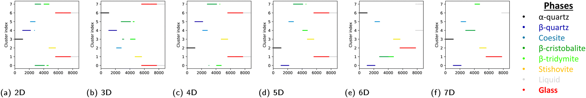 | ||
| Fig. 4 Cluster indices by k-means clustering on the projected data in low-dimensional spaces with different numbers of dimensions. The color reflects the phase of the data point. | ||
It is noteworthy that the component 6 and component 7 are essential for achieving the differentiation of the eight phases, while the component 4 and component 5 make less important contributions, if any. This suggests that the seven-dimensional space obtained by TS-LPP could be further reduced while keeping the needed information for differentiation. While such a procedure is system-dependent, it simplifies the visualization in the reduced space. In this study, the four-dimensional space obtained by keeping components 2, 3, 6, and 7 is enough to have a proper differentiation of the eight phases, and these low-dimensional spaces are indicated by the red dotted lines in Fig. 3.
3.3 Analysis of the transformation (mapping) matrices for TS-LPP
As discussed in the last section, the components 6 and 7 are important for the differentiation of the eight phases. The relationship between these components and the original LAAF dimension can be expressed by the mapping or transformation matrix explained in the ESI,† Section IIB.As the TS-LPP transformation consists of two linear transformations, the transformation matrices corresponding to each LPP step can be analyzed. Fig. 5 shows the mapping matrices for the first, second and finally the whole transformation. The components of the first LPP show that there is some degree of redundancy, as can be seen from the occurrence of several near identical columns. The second LPP mixes the components from the first LPP. Except for the final 7th component, contributions of the lower dimensional components (1st – 6th) in the intermediate dimension are large. Thus, the two-step strategy is not so relevant up to the 6th dimension. On the other hand, for final 7th component, 12th and 13th components in the intermediate dimension are important, and TS-LPP was essential for the differentiation between β-cristobalite and β-tridymite. In fact, this differentiation could not be achieved with other methods such as PCA or LPP.
 | ||
| Fig. 5 Transformation matrices for (left) the first LPP, (center) the second LPP, (right) the whole transformation. Each column is normalized. | ||
It should be noted that performing LPP to a much large number of dimension works as the relevant functions needed to capture the structural differences between β-cristobalite from β-tridymite are taken into account (ESI,† Fig. S10). However, the interpretation and visualization of such model is difficult and makes this approach less promising for future analysis of systems where the actual phase is unknown.
3.4 β-quartz to α-quartz transition
Once the linear transformation matrix is obtained by TS-LPP, new local structures which are not included in the training set can be projected onto the low-dimensional space. The model developed for differentiating all eight phases was subsequently used to analyze a trajectory starting from β-quartz and evolved at 600 K under NPT conditions. It is well known that α-quartz is the most stable phase at this temperature under atmospheric pressure (see Fig. 2). During the 5 ps run, a transition from β-quartz to α-quartz was observed. The progressive phase transition could be tracked, as shown in Fig. 6, where only components 2 and 3 of the seven-dimensional space are shown. In the initial stage (first 100 fs), the projections of the test data appear in the same region of the subspace as β-quartz (blue region in Fig. 3). In the final stage (4.9 ps to 5 ps), these points lie in the same region as α-quartz (black region in Fig. 3). Considering the whole trajectory for a selection of five atoms, a smooth transition from the β-quartz region to the α-quartz one is observed, which is captured by component 3. From Fig. 5(right), it can be seen that component 3 (third column) is mainly made of contributions from features related to Si–O distances (upper rows). | ||
| Fig. 6 Transition from β-quartz to α-quartz at 600 K followed by components 2 and 3 of the TS-LPP space. All atoms at (a) first 100 fs and (b) last 100 fs are plotted. For (c), the whole process is shown for five selected atoms. Data from the training set appear in light gray. Colors reflect the time range shown, from blue for early snapshots to red for late snapshots. | ||
So far, we have analyzed an MD simulation where the β-to-α quartz transition occurs using the low dimensional space presented in Subsection 3.2, which is based on the training data of eight phases. However, it is also possible to perform another analysis using a different low dimensional space, obtained solely from the data of a single trajectory for the β-to-α quartz transition. Here, a two-dimensional space is obtained, and the results are shown in Fig. 7. In the early stage of the simulation, the structure evolves away from its initial configuration. If the time range is large enough, the whole transition is captured as shown in Fig. 7c and d. More details can be found in the ESI.†
 | ||
| Fig. 7 Transition from β-quartz to α-quartz at 600 K followed by a TS-LPP space trained on a single trajectory, using the first (a) 100 fs, (b) 2000 fs, (c) 4000 fs and (d) 5000 fs. | ||
This demonstrates that the change of local structures can be correctly extracted in the low-dimensional space from one single MD trajectory, where the structures evolve over time.
3.5 Melt-quench process
In this case, a trajectory of a classical molecular dynamics simulation of melt and quench of silica (2592 atoms per cell) with a cooling rate of 109 K s−1 is analyzed. First, focusing on the melting part of the simulation, the structure evolves following from the α-quartz region to β-quartz, and finally liquid, as shown in Fig. 8a. By visualizing components 2, 3, 6 and 7, the evolution from one region to another can be visualized, from the blue points (initial configuration) to the red ones (final configuration). It should be noted that the transitions are quite abrupt and the melting process results in several distinct regions corresponding to different phases, quickly changing from α-quartz to β-quartz, then transitioning towards the region corresponding to the liquid phase. For the quenching process (Fig. 8b), it can be seen that the system evolves from the liquid-like region to the glass-like one in a continuous transition. No crystalline region was detected during the quench process, suggesting that the atomic structure remains disordered. | ||
| Fig. 8 Structural evolution during a melt-quench process, followed by components 2, 3, 6 and 7 of the TS-LPP space for (a) the melt part (b) the quench part. Data from the training set appear in light gray. Colors reflect the time range shown, from blue for early snapshots to red for late snapshots. | ||
4 Conclusions
We have proposed a new methodology to extract the differences in the local structures of silica system using a recently developed dimensionality reduction technique. Our approach consists of locally averaged atomic fingerprints (LAAF) based on atom-centered symmetry functions (ACSF) and using two-step locality preserving projections (TS-LPP) to generate a relatively low-dimensional space that properly catches relevant structural properties of the different phases. The targeted data set for silica system was constructed by the data points obtained from eight phases. Importantly, unlike previous works,29,31 feature selection and at least seven dimensions were needed in order to capture lower importance features that enables the proper differentiation of all phases.Our results show that proper differentiation of many phases of a given compound is possible via the combination of LAAF and an adequate dimensionality reduction. This method can be applied to any kind of material or alloy and should be independent of the simulation method (classical force fields, first-principles molecular dynamics, etc.). In the future, this knowledge should be useful for analyzing the structure of silica glass and its evolution with respect to external conditions, such as cooling rate or pressure during a quenching process. In addition, for systems such as metallic alloys, this approach could provide useful indications on the transitions that occur for instance during the glass transition, and how different factors (cooling rate, pressure, deformations, shear, etc.) can change the structural properties. In general, the present methodology should extract valuable information from inhomogeneous systems, for instance to detect the onset of nucleation in a supercooled liquid or the coexistence of several phases in different regions. By the detection of local changes, the relation between the structure and properties of atomic configurations that are typically difficult to analyze (ex: in the presence of impurities, vacancies or interfaces) could be better understood. Our methodology should therefore be applicable to inhomogeneous systems where phases may coexist or during nucleation in a supercooled liquid.
Our method is unsupervised, thus does not rely on any biased information, and is promising for detecting particular phases or local structures, which may appear in any kind of material, as well as detecting new unknown phases dynamically or density fluctuations.4 Used as a supervised learning method, for classification, it may be a stepping stone towards better machine learning potentials or force fields50,51 by allowing classification of the atoms beforehand and choosing an appropriate force field for each atom over the course of a simulation.
Author contributions
A. Lu: conceptualization, data curation, methodology, formal analysis, writing – original draft. J. Lin: formal analysis. Y. Futamura: formal analysis. T. Sakurai; formal analysis, writing – review and editing. R. Tamura: methodology, formal analysis, writing – review and editing. T. Miyazaki: conceptualization, funding acquisition, supervision, formal analysis, writing – review and editing.Data availability
The data of this study are available from the corresponding authors upon reasonable request.Conflicts of interest
There are no conflicts to declare.Appendices
A Descriptors
In order to capture the structural differences in silica, descriptors based on atom-centered symmetry functions were defined. | (1) |
 | (2) |
| Vi(rd) = (Vi(η1;rd),Vi(η2;rd),…,Vi(ηM;rd)). | (3) |
 | (4) |
 | (5) |
And the fingerprint vector becomes 2M-dimensional:
| Vi∈a(rd) = (Vai∈a(η1;rd), …, Vai∈a(ηM;rd), Vbi∈a(η1;rd), …, Vbi∈a(ηM;rd)). | (6) |
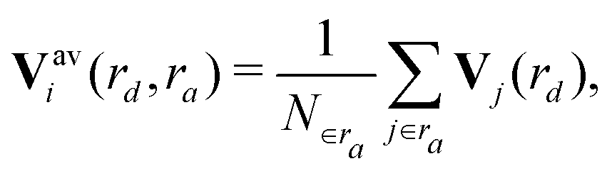 | (7) |
 | (8) |
There are two important distance cutoff values:
1. rd: the distance cutoff for the descriptor.
2. ra: the distance cutoff for locally averaging the descriptor.
These values were carefully chosen so that the characteristics of each phase are properly captured. In this work rd = ra = 6 Å.
Finally, feature selection based on variance threshold (10−4) and standardization were performed on the resulting LAAF vector to obtain unit variance. This lead to a reduction of the number of features from 100 to 63.
B Dimensionality reduction
First, a weighted adjacency matrix W is defined as:
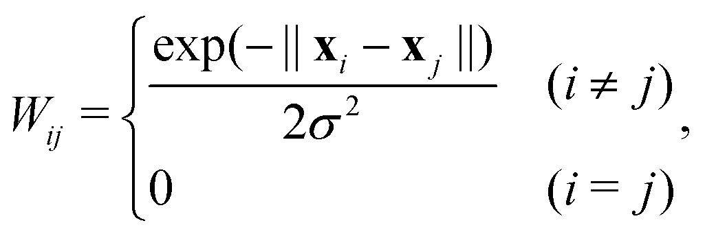 | (9) |
Next, the knn-nearest neighbor graph is created. A typical value is knn = 7. This similarity graph is based on W, where the off-diagonal elements are forced to zero, except for those related to the knn nearest neighbor data points. The weighted adjacency matrix is made symmetric by the operation56
| Wij = max(Wij,Wji). | (10) |
The square diagonal matrix D, called the degree matrix, is defined as:
 | (11) |
 | (12) |
The graph Laplacian is defined as:
| L = D−W. | (13) |
| XTLXy = λXTDXy, | (14) |
For a target dimension dr, the mapping matrix Y by LPP from M to dr dimensions is obtained by
| Y = (y1, y2,…, ydr). | (15) |
| x′ = xY | (16) |
Acknowledgements
The computations in the present work were performed on the Numerical Materials Simulator at the National Institute for Materials Science. This study was supported by the JSPS Grant-in-Aid for Transformative Research Areas (A) ‘Hyper-Ordered Structures Science’ (Grant No. 20H05883) and the JSPS Grant-in-Aid for Scientific Research (Grant No. 18H01143, 21H01008).References
- M. Mazloom, A. Ramezanianpour and J. Brooks, Cem. Concr. Compos., 2004, 26, 347–357 CrossRef CAS.
- A. J. Ikushima, T. Fujiwara and K. Saito, J. Appl. Phys., 2000, 88, 1201–1213 CrossRef CAS.
- J. E. Lilienfeld, Method and apparatus for controlling electric currents, 1930, https://patents.google.com/patent/US1745175A/en.
- G. N. Greaves and S. Sen, Adv. Phys., 2007, 56, 1–166 CrossRef CAS.
- G. Hart, J. Mineral. Soc. Am., 1927, 12, 383–395 Search PubMed.
- G. A. Lager, J. D. Jorgensen and F. J. Rotella, J. Appl. Phys., 1982, 53, 6751–6756 CrossRef CAS.
- A. Wright and M. Lehmann, J. Solid State Chem., 1981, 36, 371–380 CrossRef CAS.
- L. Levien and C. T. Prewitt, Am. Mineral., 1981, 66, 324–333 CAS.
- E. C. T. Chao, J. J. Fahey, J. Littler and D. J. Milton, J. Geophys. Res., 1962, 67, 419–421 CrossRef CAS.
- E. Ringdalen, JOM, 2014, 67, 484–492 CrossRef.
- M. Kayama, H. Nagaoka and T. Niihara, Minerals, 2018, 8, 267 CrossRef.
- R. Car and M. Parrinello, Phys. Rev. Lett., 1985, 55, 2471–2474 CrossRef CAS PubMed.
- R. Car and M. Parrinello, Phys. Rev. Lett., 1988, 60, 204–207 CrossRef CAS PubMed.
- F. H. Stillinger and T. A. Weber, Phys. Rev. A: At., Mol., Opt. Phys., 1982, 25, 978–989 CrossRef CAS.
- S.-H. Lee, J. Kim, S.-J. Kim, S. Kim and G.-S. Park, Phys. Rev. Lett., 2013, 110, 235502 CrossRef PubMed.
- K. Nishio, T. Miyazaki and H. Nakamura, Phys. Rev. Lett., 2013, 111, 155502 CrossRef PubMed.
- H. Tong and H. Tanaka, Phys. Rev. X, 2018, 8, 011041 CAS.
- A. P. Bartók, R. Kondor and G. Csányi, Phys. Rev. B: Condens. Matter Mater. Phys., 2013, 87, 184115 CrossRef.
- S. V. King, Nature, 1967, 213, 1112–1113 CrossRef CAS.
- S. Le Roux and P. Jund, Comput. Mater. Sci., 2010, 49, 70–83 CrossRef CAS.
- S. L. Roux and P. Jund, Comput. Mater. Sci., 2011, 50, 1217 CrossRef.
- Y. Hiraoka, T. Nakamura, A. Hirata, E. G. Escolar, K. Matsue and Y. Nishiura, Proc. Natl. Acad. Sci. U. S. A., 2016, 113, 7035–7040 CrossRef CAS PubMed.
- Y. Onodera, S. Kohara, P. S. Salmon, A. Hirata, N. Nishiyama, S. Kitani, A. Zeidler, M. Shiga, A. Masuno, H. Inoue, S. Tahara, A. Polidori, H. E. Fischer, T. Mori, S. Kojima, H. Kawaji, A. I. Kolesnikov, M. B. Stone, M. G. Tucker, M. T. McDonnell, A. C. Hannon, Y. Hiraoka, I. Obayashi, T. Nakamura, J. Akola, Y. Fujii, K. Ohara, T. Taniguchi and O. Sakata, NPG Asia Mater., 2020, 12, 1–16 CrossRef.
- J. Konnert, P. D'Antonio and J. Karle, J. Non-Cryst. Solids, 1982, 53, 135–141 CrossRef CAS.
- F. Li and J. S. Lannin, Phys. Rev. Lett., 1990, 65, 1905–1908 CrossRef CAS PubMed.
- N. Lačević, F. W. Starr, T. B. Schrøder, V. N. Novikov and S. C. Glotzer, Phys. Rev. E: Stat., Nonlinear, Soft Matter Phys., 2002, 66, 030101 CrossRef PubMed.
- J. D. Honeycutt and H. C. Andersen, J. Phys. Chem., 1987, 91, 4950–4963 CrossRef CAS.
- A. K. A. Lu and D. V. Louzguine-Luzgin, J. Chem. Phys., 2022, 157, 014506 CrossRef CAS PubMed.
- W. Lechner and C. Dellago, J. Chem. Phys., 2008, 129, 114707 CrossRef PubMed.
- P. M. Piaggi and M. Parrinello, J. Chem. Phys., 2017, 147, 114112 CrossRef PubMed.
- R. Tamura, M. Matsuda, J. Lin, Y. Futamura, T. Sakurai and T. Miyazaki, Phys. Rev. B, 2022, 105, 075107 CrossRef CAS.
- J. Behler, J. Chem. Phys., 2011, 134, 074106 CrossRef PubMed.
- T. Caliński and J. Harabasz, Commun. Stn., 1974, 3, 1–27 Search PubMed.
- CONQUEST: Linear Scaling DFT, https://ordern.github.io/, (accessed March 2024).
- D. R. Bowler, R. Choudhury, M. J. Gillan and T. Miyazaki, Phys. Status Solidi B, 2006, 243, 989–1000 CrossRef CAS.
- A. Nakata, J. S. Baker, S. Y. Mujahed, J. T. L. Poulton, S. Arapan, J. Lin, Z. Raza, S. Yadav, L. Truflandier, T. Miyazaki and D. R. Bowler, J. Chem. Phys., 2020, 152, 164112 CrossRef CAS PubMed.
- J. P. Perdew, K. Burke and M. Ernzerhof, Phys. Rev. Lett., 1996, 77, 3865–3868 CrossRef CAS PubMed.
- D. R. Hamann, Phys. Rev. B: Condens. Matter Mater. Phys., 2013, 88, 085117 CrossRef.
- M. van Setten, M. Giantomassi, E. Bousquet, M. Verstraete, D. Hamann, X. Gonze and G.-M. Rignanese, Comput. Phys. Commun., 2018, 226, 39–54 CrossRef CAS.
- D. R. Bowler, J. S. Baker, J. T. L. Poulton, S. Y. Mujahed, J. Lin, S. Yadav, Z. Raza and T. Miyazaki, Jpn. J. Appl. Phys., 2019, 58, 100503 CrossRef CAS.
- G. J. Martyna, M. L. Klein and M. Tuckerman, J. Chem. Phys., 1992, 97, 2635–2643 CrossRef.
- M. Parrinello and A. Rahman, J. Appl. Phys., 1981, 52, 7182–7190 CrossRef CAS.
- S. Plimpton, J. Comput. Phys., 1995, 117, 1–19 CrossRef CAS.
- W. M. Brown, P. Wang, S. J. Plimpton and A. N. Tharrington, Comput. Phys. Commun., 2011, 182, 898–911 CrossRef CAS.
- S. Munetoh, T. Motooka, K. Moriguchi and A. Shintani, Comput. Mater. Sci., 2007, 39, 334–339 CrossRef CAS.
- G. J. Martyna, D. J. Tobias and M. L. Klein, J. Chem. Phys., 1994, 101, 4177–4189 CrossRef CAS.
- W. Shinoda, M. Shiga and M. Mikami, Phys. Rev. B: Condens. Matter Mater. Phys., 2004, 69, 134103 CrossRef.
- J. Lin, R. Tamura, Y. Futamura, T. Sakurai and T. Miyazaki, Phys. Chem. Chem. Phys., 2023, 25, 17978–17986 RSC.
- M. Ester, H.-P. Kriegel, J. Sander and X. Xu, Proceedings of the Second International Conference on Knowledge Discovery and Data Mining, 1996, p. 226–231.
- J. Behler, J. Chem. Phys., 2016, 145, 170901 CrossRef PubMed.
- R. Tamura, J. Lin and T. Miyazaki, J. Phys. Soc. Jpn., 2019, 88, 044601 CrossRef.
- J. Behler and M. Parrinello, Phys. Rev. Lett., 2007, 98, 146401 CrossRef PubMed.
- K. Pearson, London, Edinburgh Dublin Philos. Mag. J. Sci., 1901, 2, 559–572 CrossRef.
- H. Hotelling, Biometrika, 1936, 28, 321–377 CrossRef.
- X. He and P. Niyogi, Proceedings of the 16th International Conference on Neural Information Processing Systems, Cambridge, MA, USA, 2003, p. 153–160.
- U. von Luxburg, Stat. Comput., 2007, 17, 395–416 CrossRef.
- F. Pedregosa, G. Varoquaux, A. Gramfort, V. Michel, B. Thirion, O. Grisel, M. Blondel, P. Prettenhofer, R. Weiss, V. Dubourg, J. Vanderplas, A. Passos, D. Cournapeau, M. Brucher, M. Perrot and E. Duchesnay, J. Mach. Learn. Res., 2011, 12, 2825–2830 Search PubMed.
Footnote |
| † Electronic supplementary information (ESI) available. See DOI: https://doi.org/10.1039/d3cp06298h |
| This journal is © the Owner Societies 2024 |