Electron doping as a handle to increase the Curie temperature in ferrimagnetic Mn3Si2X6 (X = Se, Te)†
Received
14th November 2023
, Accepted 23rd January 2024
First published on 31st January 2024
Abstract
By analysing the results of ab initio simulations performed for Mn3Si2X6 (X = Se, Te), we first discuss the analogies and the differences in electronic and magnetic properties arising from the anion substitution, in terms of size, electronegativity, band widths of p electrons and spin–orbit coupling strengths. For example, through mean-field theory and simulations based on density functional theory, we demonstrate that magnetic frustration, known to be present in Mn3Si2Te6, also exists in Mn3Si2Se6 and leading to a ferrimagnetic ground state. Building on these results, we propose a strategy, electronic doping, to reduce the frustration and thus to increase the Curie temperature (TC). To this end, we first study the effect of electronic doping on the electronic structure and magnetic properties and discuss the differences in the two compounds, along with their causes. Secondly, we perform Monte-Carlo simulations, considering from the first to the fifth nearest–neighbor magnetic interactions and single-ion anisotropy, and show that electron doping efficiently raises the TC.
1 Introduction
Mn3Si2Se6 (MSS) and Mn3Si2Te6 (MST)1,2 represent two sister compounds, halfway between two-dimensional (2D) and three-dimensional (3D) materials; in fact, they are formed by (i) a 2D Mn2Si2X6 (X = Se, Te) layer, in all respects equivalent to one of the prototypical 2D magnets, i.e. Cr2Ge2Te6;3 (ii) a Mn intercalating layer, forming a triangular lattice, placed in the so called “van der Waals gap” of bulk 2D-magnets and granting a 3D behaviour to this class of materials. MSS and MST have been studied by numerous researchers in recent years.1,4–7 MST features polaronic transport and very low values of thermal conductivity, which is further suppressed in magnetic field.6 The resistivity decreases by 7 orders of magnitude when the MST is placed in a magnetic field greater than 9 T, leading to an insulator–metal transition at 130 K.8 Zhang et al. also proposed to regulate the metal–insulator transition by spin orientation and Se instead of Te.7 Sala et al. systematic studied the magnetic frustration state in the MST by combining experiments and calculations.9 Wang et al. demonstrated that at a pressure of 10 GPa, the TC of MST can be increased to 210 K while maintaining the ferrimagnetic ground state.10 MSS and MST are isomorphic compounds, hence they are expected to feature similar properties. Among them, we recall the ground state of both MSS and MST being ferrimagnetic with 5μB magnetic moments and opposite direction of Mn1 and Mn2 sublattices, resulting in a net magnetic moment of 1.6μB per Mn.1,2 The antiferromagnetic (AFM) coupling between Mn atoms and the competition between different nearest neighbors leading to the interesting ferrimagnetic configuration in MST2,11 is also expected to play a role in MSS. There are also some differences between MSS and MST, mostly induced by the different ionicity and size of the anion, but also to the magnitude of spin orbit coupling (SOC) in the telluride and in the selenide. The current doubt lies in the magnetization direction of MSS and MST. Multiple experiments and calculations believe that the two materials have in-plane magnetization.1,6–8,11–13 However, some researchers have proposed that the magnetization directions of MSS and MST have angles of around 35° and 10° with the ab plane respectively.2,14 Our calculation results more support the former statement.
A magnet ideal for applications should possess several properties, such as strong magnetocrystalline anisotropy, quantum anomalous Hall effect, perfect crystalline order, high TCetc.15 In particular, great efforts were directed towards increasing the ordering temperature of magnetic materials whenever their TC is far below room-temperature. Different routes were followed, among which the most common are represented by external fields,16,17 intercalation,18 strain engineering,19 molecule absorption20–23 and formation of heterostructures with other materials.24–27 In this respect, we note that the TC of MSS is 67 K, which is slightly lower than 78 K of MST2,10,11 It is therefore obvious that such low TCs limit the range of applications of these materials and increasing the TC appears vital for their use in spintronic devices.
In our previous work,28 we focused on magnetic properties in MST, by means of a joint theoretical and experimental study. In addition to pointing to a strong covalency between Mn and Te states, we highlighted the mechanism by which the magnetic frustration in MST eventually leads to a ferrimagnetic ground state, and demonstrate a crucial role of both exchange interactions extending beyond nearest–neighbours and of anti-symmetric exchange in dictating its TC.
In this work, we systematically investigate the electronic structure and the magnetic properties of MSS and MST, by discussing the differences between the two materials, mostly in terms of (i) different ionicity and size of the anion; (ii) SOC strengths. Importantly, we put forward electronic doping as an efficient tool to largely increase the TC of MSS and MST; by decreasing the exchange frustration, our results show that electron doping stabilizes ferromagnetism in the Mn1 plane. The mean-field (MF) theory and the Monte-Carlo (MC) simulations – based on a spin-Hamiltonian which also takes into account the single-ion anisotropy, with all parameters evaluated from first-principles – show that electron doping can effectively increase the TC. Based on MC simulations, up to 250 K and 140 K are reached for MST and MSS, respectively, for a doping of 0.8 electrons per unit-cell.
2 Methods
2.1 Density functional theory
Density functional theory (DFT) calculations were performed within the generalized gradient approximation (GGA)29 in the form proposed by Perdew–Burke–Ernzerhof (PBE), as implemented in the Vienna ab Initio Simulation Package (VASP).30 An additional on-site interaction was considered within a DFT+U approach in the form introduced by Dudarev et al.31 From our previous study28 focused on an accurate comparison between DFT and spectroscopy experiments, U = 2 eV appeared to be the best choice in the description of electronic and magnetic properties, that is, we only use different U values for Section 3. The projector augmented wave (PAW) pseudopotentials32,33 were used, considering as valence states 3p63d54s2 for Mn, 3s23p2 for Si, 4s24p4 for Se and 5s25p4 for Te. The plane-wave energy cutoff was fixed to 600 eV. The convergence criterion for total energy differences during the self-consistent cycle was set to less than 10−6 eV and the threshold on the maximum force on each ion was less than 0.005 eV Å−1. It should be noted that the lattice constants from experiments are used for MST, while the DFT-optimized lattice parameters of MSS (for which, to the best of our knowledge, no experimental data are available) are adopted: a = 6.544 Å, c = 13.724 Å for MSS and a = 7.028 Å, c = 14.255 Å for MST. We note that for MST the difference between DFT-predicted (a = 7.079 Å, c = 14.332 Å) and experimental values is smaller than 1% (i.e. a standard accuracy for DFT predictions) and we therefore expect a careful description of structural properties also for MSS. The magnetic anisotropic energy (MAE) was calculated by taking into consideration SOC. We chose the 6 × 6 × 4 Γ-centered k-grid sampling34 for the unit-cell. The four-state method35 was used for the evaluation of the exchange-coupling constants and single-ion anisotropy. In that case, for the 2 × 2 × 1 supercell used in the calculation of single ion anisotropy (SIA) and for the 3 × 3 × 1 supercell used in the calculation of exchange constants, we chose a 2 × 2 × 2 k-grid sampling. The electronic doping is modeled by artificially changing the number of electrons in the unit-cells and considering an homogeneous background-charge.
2.2 Monte-Carlo
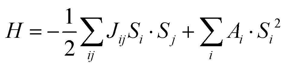
The magnetic properties can be modeled via a spin model for classical spins, including a pair-wise spin–spin scalar Heisenberg coupling and a SIA term:| |  | (1) |
where Jij is the magnetic exchange parameter between Si and Sj. We used the VAMPIRE36 code to perform MC simulations, assuming isotropic exchange constants up to the fifth nearest neighbor; anisotropic effects are modeled via an effective SIA term with coupling constant Ai extracted from MAE. The standard Metropolis algorithm37 has been used for MC simulations with 5 × 10⁴ MC steps for equilibrium and 1 × 10⁵ MC steps for averaging. Since the VAMPIRE software can only simulate cuboid cells, we used 1 × √3 × 1 cells, which contains eight Mn1 and four Mn2 sites. We performed calculations for a 16 × 8 × 6 supercell with Ns = 10![[thin space (1/6-em)]](https://www.rsc.org/images/entities/char_2009.gif) 368 spins. The transition temperature can be estimated from the peaks that appear in the temperature evolution of specific heat, evaluated as:
368 spins. The transition temperature can be estimated from the peaks that appear in the temperature evolution of specific heat, evaluated as:
where E is the energy calculated using model eqn (1), kB is the Boltzmann constant and β = 1/kBT, while 〈…〉 indicates statistical averages.
3 Results and discussion for pristine MSS and MST compounds
3.1 Band structures
Before starting the discussion of the electronic properties, let us recall that the unit cell of MSS and MST, as shown in Fig. 1(a), in the P![[3 with combining macron]](https://www.rsc.org/images/entities/char_0033_0304.gif) 1c phase (space group no. 163) comprises 6 Mn atoms, each carrying a local magnetic moment: there are two symmetry-inequivalent manganese atoms belonging to 4f and 2c Wyckoff positions. The Se (Te) atoms occupy 12i Wyckoff positions in MSS (MST). Each Mn atom is at the center of a tilted octahedron composed of Se/Te, with Mn1-centered octahedra sharing edges with octahedra around Mn1 and sharing faces with the octahedra around Mn2.
1c phase (space group no. 163) comprises 6 Mn atoms, each carrying a local magnetic moment: there are two symmetry-inequivalent manganese atoms belonging to 4f and 2c Wyckoff positions. The Se (Te) atoms occupy 12i Wyckoff positions in MSS (MST). Each Mn atom is at the center of a tilted octahedron composed of Se/Te, with Mn1-centered octahedra sharing edges with octahedra around Mn1 and sharing faces with the octahedra around Mn2.
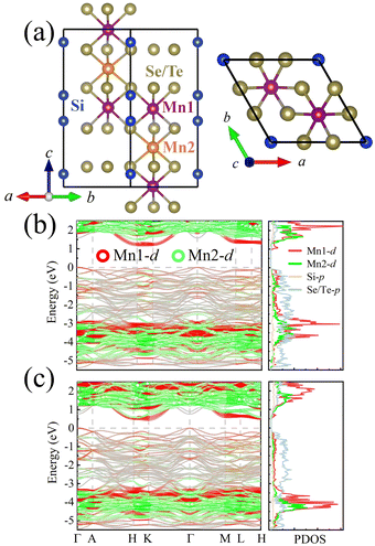 |
| | Fig. 1 (a) MSS and MST structures. Side (top) view on the left (right) panel. Legend for atomic colors: Mn1-purple, Mn2-orange, Si-blue, Se or Te-yellow. Band structure and corresponding projected density of states of (b) MSS and (c) MST, respectively (calculated with effective U = 2 eV). | |
Fig. 1(b) and (c) show the band structures and density of states (DOS) of MSS and MST, which are characterized as indirect bandgap semiconductors with bandgap of 1.19 and 0.45 eV, respectively. These values are obtained within DFT, so they are likely underestimated with respect to experimental values, due to the well known failure of DFT in treating excited states.38 As expected from the larger electronegativity of Se with respect to Te, MSS shows a stronger insulating behaviour with respect to MST. To further understand the electronic structure, we show the band structures in Fig. 1(b) and (c) taking into account their orbital character; in particular, Mn1- and Mn2-derived states are represented by red and green, respectively. Se/Te gives rise to most of the states near the valence band maximum, while the d electrons of Mn mostly occupy somewhat deeper energy levels, i.e., the energy range of −5 to −3 eV. Interestingly, we find that the conduction band minimum (CBM) is mostly contributed by Mn1, with Si and Se/Te also contributing partly, and only Mn2 not contributing at all. The difference in electronic structure between Mn1 and Mn2 suggests that, when doping with electrons, these latter are more likely to move in the plane containing Mn1 octahedra, rather than in the plane of Mn2 octahedra. This behaviour will be particularly important when discussing below the dependence of the exchange parameters upon doping (see Section 4).
As noted previously for MST,11 the band gap can be largely modulated by the magnetic moments orientation, as shown in Fig. S1 (ESI†). Due to the nodal-line degeneracy protected by the underlying symmetry, the valence band at the Γ point splits into two bands when MSX have out-of-plane magnetization. This effect is present in both MSS and MST, with a splitting size of 0.16 and 0.38 eV for MSS and MST, respectively. The smaller magnitude in MSS suggests the SOC strength to be the key parameter in the band gap modulation, consistently with previous reports.11
3.2 Exchange coupling constants
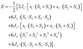
Here, we start discussing the magnetic properties of MSS and MST. We denote as Si and sj in eqn (1) for Mn1 and Mn2, respectively (with i = 1,…,4 and j = 1, 2), the classical spins that describe the magnetic moments of the two sets of Mn. Assuming up to third nearest neighbor interactions and an isotropic Heisenberg model for classical spins [i.e., neglecting the anisotropic term in eqn (1)], the energy per cell reads:| |  | (2) |
As displayed in Fig. 2(c), J1, J3 describe interlayer coupling between S1 and sj spins, whereas J2 is the intralayer coupling between Si spins. It should be noted that we consider S = s = 5/2 in this work. By considering five different spin configurations, as shown in Fig. 2(a), we obtain the following equations:
| EFI1 = +4J1 − 6J2 + 12J3 + E0 |
| EAF1 = −4J1 + 6J2 + 12J3 + E0 |
| EAF2 = +4J1 + 6J2 − 12J3 + E0 |
| | | EFM = −4J1 − 6J2 − 12J3 + E0 | (3) |
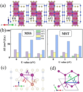 |
| | Fig. 2 (a) Schematic representation of the different magnetic configurations used in energy-mapping method (FM not shown here). (b) Energy difference between different magnetic configurations of MSS (left panel) and MST (right panel), respectively. As the effective U value increases, the energy difference decreases. (c) and (d) Schematic diagrams of first nearest neighbor to fifth nearest neighbor. Panel (c) shows a side-view, whereas (d) shows a top-view of the Mn1 plane. | |
The best-fit solutions of exchange parameters from eqn (3) are shown in Table 1. For both MSS and MST, all the interactions between Mn spins are negative, i.e. corresponding to an AFM interaction. As shown in Table 1, the magnetic interaction decreases as the U value increases. This is consistent with superexchange theory, according to which the exchange interaction goes as t2/U, where t represents a hopping parameter. Within this simple picture, the larger the U value, the more localized the electrons, the smaller the exchange interaction. The exchange parameters of MST are basically the same as previously reported.1,7,9,11 The in-plane AFM exchange interactions indicate that the exchange paths between different nearest neighbors are frustrated in the ferrimagnetic ground state. In fact, the J1 and J3 drive antiferromagnetic interactions between Mn1 and Mn2 atoms, while J2 would lead to antiferromagnetic interactions between Mn1 atoms and competing with the desired action of J1 and J3. The final ferrimagnetic ground state however shows that the “competition is won” by interplanar AFM exchange interactions, since both J1 and J3 are larger than J2.
Table 1 Exchange parameters (in meV) of MSS and MST, calculated with different effective U values and different methods (energy-mapping vs. four-state). Note that a and b represent the energy-mapping method and four-state method for solving the exchange interaction. Negative values denote an antiferromagnetic interaction
|
|
Method |
U (eV) |
J
1
|
J
2
|
J
3
|
|
a = energy-mapping method, b = four-state method. |
| MSS |
a
|
0 |
−3.71 |
−2.3 |
−2.36 |
|
a
|
1 |
−2.70 |
−1.60 |
−1.69 |
|
a
|
2 |
−2.04 |
−1.15
|
−1.20 |
|
b
|
2 |
−1.92 |
−0.69 |
−1.11 |
|
|
| MST |
a
|
0 |
−5.72 |
−1.84 |
−2.27 |
|
a
|
1 |
−4.59 |
−1.36 |
−1.72 |
|
a
|
2 |
−3.53 |
−0.88
|
−1.20 |
|
b
|
2 |
−3.19 |
−0.38 |
−1.01 |
|
|
J
4
|
J
5
|
J
2 + J5 |
| MSS |
b
|
2 |
−0.08 |
−0.28 |
−0.97
|
| MST |
−0.08 |
−0.26 |
−0.64
|
Heisenberg spin exchange parameters can also be evaluated by using the four-state method.35 As shown in Table 1, we calculate even longer distance exchange parameters, that is from J1 to J5, as shown in Fig. 2(c) and (d). It is clear that for J1 and J3 the two methods give similar results. However, for J2, the results of the two methods are quite different, with the results of MSS and MST differing by 67% and 130%. Actually, this difference comes from the used methodology itself. In fact, the hexagon plane formed by the Mn1 atoms contains three J2, six J4 and three J5 interactions for each Mn1, which in turn is shared among three hexagons, and the energy per cell reads:
| |  | (4) |
On the other hand, when describing the hexagon plane formed by the Mn1 atoms by a single J2, the latter effectively contains also longer-ranged exchange interactions (not explicitly taken into account). Clearly, the J4 exchange constant cannot be evaluated from the energy-mapping method, as it gives a constant contribution for any magnetic configuration that can be described within the unit cell. By comparing eqn (2) and (4), it is also evident that the J2 estimated within the energy-mapping method effectively includes contribution from fifth nearest neighbor and should be compared with J2 + J5 as obtained from the four-state method.
Based on the above relations and Table 1, we find that the difference between the “effective” J2 (from the mapping-method) and J2 + J5 (from the four-state method) is indeed quite close. From the perspective of the exchange constant, for both MSS and MST we also get the same conclusion as our previous work, that is, the importance of explicitly including J4 and J5, when calculating magnetic properties.28
3.3 Magnetic anisotropy energy and band-gap: dependence on Hubbard-U parameter
In addition to the magnetic exchange interactions, other relevant properties of MSS and MST, such as MAE and band gap, are also sensitive to U. As shown in Fig. 3(c), the MAE of MSS and MST decreases significantly as the value of U increases. The MAE of MSS is smaller than that of MST, as expected from the weaker SOC effect of Se compared to Te. This is similar to what obtained in the comparison of MAE in CrBr3 and CrI3.39 According to our DFT predictions, both MSS and MST prefer in-plane magnetization. Zhang et al. claim that the system maintains the in-plane magnetization during the substitution of Se for Te up to 30% concentration, which somewhat implies that MSS will also be in-plane magnetization.7 From this point, our calculations are consistent. However, May et al. claim the magnetization direction of MSS is rotated by 35° with respect to the xy plane.2 The reason for the discrepancy is unclear.
 |
| | Fig. 3 (a) Dependence of the DFT band gap on the effective U values. (b) Schematic diagram of magnetic moments direction. An angle θ equal to 0° and 90° represent the direction of magnetization lying in the xy plane and along the z axis, respectively. (c) Angular dependence of the magnetocrystalline anisotropy energy of MSS (left panel) and MST (right panel). Different color lines are calculated with different effective U values. It should be noted that during the process of magnetization rotation from in-plane to out-of-plane, the antiparallel configuration between Mn1 and Mn2 magnetic moments is preserved. | |
For the band gap, the larger the U value, the larger the band gap. In closer detail, in the range of U from 0 to 5 eV, the DFT band gap of MSS changes in the range from 0.61 to 1.74 eV; MST goes from a metal to semiconductor with a band gap of 0.82 eV. The behaviour of the band gap as a function of the Hubbard U parameter is expected from the situation of a half-filled d shell, as the one we have here for Mn d5. Indeed, as the (empty) CBM is predominantly contributed by Mn1 d states, it shifts up in energy as U increases, thereby leading to a band-gap opening. The experimental band gap of MST is 1.39 eV,40 while the band gap of MSS has not yet been experimentally published. Based on the difference in electronegativity between Se and Te element, it can be predicted that the experimental band gap of MSS is larger than that of MST.
3.4 Mean-field analysis
Next, we derive the effective Weiss field generated on each magnetic moment in the cell (representative of a given sublattice) by all surrounding atoms to obtain the critical temperature. The Weiss fields are,
| B1 = J1m1 + 3J2M2 + 3J3m2 |
| B2 = J1m2 + 3J2M1 + 3J3m1 |
| B3 = J1m1 + 3J2M4 + 3J3m2 |
| B4 = J1m2 + 3J2M3 + 3J3m1 |
| b1 = J1(M1 + M3) + 3J3(M2 + M4) |
| | | b2 = J1(M2 + M4) + 3J3(M1 + M3) | (5) |
where each expectation value Mi = 〈Si〉 and mi = 〈si〉 satisfies the self-consistent equation for a classical spin:| |  | (6) |
with β = 1/(kBT). The right-hand side approximation holds in the limit of βBi → 0 when T is close to TC. Combining eqn (5) and (6), the following equations for the sublattice magnetizations  and
and  can be obtained:
| |  | (7) |
The following quadratic equation is readily derived:
| |  | (8) |
using which the critical temperature is obtained as:
| |  | (9) |
where sgn
J2 =
J2/|
J2| denotes the sign of the
J2 exchange parameter. The physically meaningful solution of a Curie temperature larger than 0 implies that only the positive result from
eqn (9) is retained. Taking into account interactions for longer distances, one can still use MF theory to estimate the critical temperature. By repeating the above derivation process, one obtains:
| | 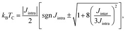 | (10) |
where we defined intra- and inter-sublattice effective exchange parameters
Jintra =
J2 + 2
J4 +
J5 and
Jinter =
J1 + 3
J3, respectively.
4 Results and discussion on the effects of electronic doping
Our recipe for the increase in TC starts from the following consideration. As previously discussed, in both MSS and MST J2, J4 and J5 predict an AFM interaction between Mn1, i.e. they have an opposite effect with respect to J1 and J3; in other words, the competing effects driven by J2, J4 and J5 reduce the stability of the ferrimagnetic configuration and thus the TC. We mentioned that CBM is contributed by Mn1 in band structure part, in the case of light doping, electrons will first move in the Mn1 plane, which is likely to change the exchange parameters of Mn1 plane, that are J2, J4 and J5, thus change the magnetic frustration state. Here we propose a route to increase the TC by weakening the competition between the magnetic interactions and let them cooperate one with the other to improve the stability of the ferrimagnetic state: tuning the intensity of exchange parameters by electron doping. The latter obviously induces a change from semiconducting to metallic behaviour, along with other less-trivial property changes, which we are going to discuss in detail in this section.
4.1 Trends of exchange constants vs. doping
Fig. 4(a) and (b) shows the response of the magnetic exchange parameters of MSS and MST to electron doping. Remarkably, J2 is predicted to be extremely sensitive to the doping concentration and changes from AFM to FM as the doping concentration increases, while J1 and J3 remain basically unchanged; this situation exactly corresponds to the weakening of the competing antiferromagnetic interactions and to the emergence of ferromagnetic interactions between Mn1 atoms. In other words, J2 no longer competes with J1 and J3, but rather helps J1 and J3 to establish the ferromagnetic order in the Mn1 plane, which is expected to increase the TC. It should be noted that J4 and J5 – which are also interactions occurring within the Mn1 plane – have a weaker effect on the TC with respect to J2 in the undoped case, and their sensitivity to the doping concentration is far lower than that of J2.
 |
| | Fig. 4 Electronic doping effect on exchange parameters of (a) MSS and (b) MST. Black, blue, green and purple triangles show J1, J3, J4 and J5, respectively. J2 is shown in red filled circles, to highlight its importance related to the sign change from AFM to FM upon doping. | |
Additionally, it is noteworthy that the responses of J4 and J5 of MSS and MST diverge when the doping concentration exceeds 0.8 e per unitcell. Given the similarities between MSS and MST, we think that this discrepancy may stem from the limitations of our approximations (i.e., homogeneous electron doping, validity of Heisenberg-like short-ranged interactions, etc.), which may only be valid for low levels of electron doping. Consequently, all subsequent calculations are considered up to a doping concentration of 0.8 e per unitcell.
4.2 Trends of total magnetization per unit cell vs. doping
As known from the previous discussion of the band structures (cfr Fig. 1), the doped electrons will fill minority Mn1 levels, thereby reducing the moments on Mn1. This will globally result in a linear decrease of the total magnetic moment per unit-cell from the value in the undoped case, i.e. 1.667μB per Mn or to say 10μB per unitcell, as shown in Fig. 5(a). Notably, the magnetic moments of MSS and MST change linearly with the same trend for small doping levels. However, there is a difference between MSS and MST when the electron concentration becomes larger than 0.3 e per unitcell, leading to a non-linear behaviour in MST.
 |
| | Fig. 5 The electronic doping effect in MSS and MST on (a) MAE (left y-axis) and magnetic moment (right y-axis), (b) single ion anisotropic energy in Mn1 and Mn2. | |
One can understand the non-linear behavior from the band structure projected on Mn1 and Mn2 at different doping concentrations in Fig. S2 (ESI†). Electron doping is essentially raising the energy corresponding to the Fermi level. In MSS, the Fermi energy level with different doping concentrations only crosses the bands due to Mn1, i.e. the doped electrons reduce the magnetic moments of Mn1 atoms, keeping the Mn2 magnetic moments constant; as a result, there is a linear reduction of the total magnetization per unit cell due to the ferrimagnetic ordering, to be ascribed to the reduction of Mn1 moments. On the other hand, in MST, the Fermi energy level crosses the bands of both Mn1 and Mn2 even for small doping concentrations. The doped electrons are therefore reducing the magnetic moment of both Mn1 and Mn2; due to the ferrimagnetic arrangement and to the complex band structure effects with different filling of Mn1 and Mn2 minority-spin bands, the change in the magnetic moment per unit cell is no longer linear when increasing the doping concentration.
4.3 Trends of magnetic anisotropy
As shown in Fig. 5(a), electron doping also strongly weakens the magnetic anisotropy, i.e. it greatly reduces the energy difference between in-plane magnetization and out-of-plane magnetization. In principle, given the observed trend, electron doping could even lead to a switch from in-plane to out-of-plane anisotropy for large doping levels, as in Mn2Ge2Te6 with similar phenomena.41
We note from Fig. 5(a) that the rate of reduction of the MAE energy difference is higher for MST than for MSS. We recall that MAE is composed by two different contributions, one related to the SIA and the other to symmetric anisotropic exchange, the latter being about 15% of the total MAE in undoped MST.28 However, the discussion here will be limited to the behaviour of SIA upon doping, as the evaluation of anisotropic exchange (i.e. of off-diagonal components of the exchange tensor evaluated estimated from large supercells) would be too CPU-time-consuming to perform for all the doping levels. Based on the different site-symmetry of Mn1 and Mn2, we focus on the SIA of both separately, with the results shown in Fig. 5(b). There are two interesting points to notice. Firstly, the SIA of Mn1 in MSS is bigger than that of Mn1 in MST, while the opposite is true for Mn2 in MSS and MST. The second and interesting point is that the SIA of Mn1 is much more sensitive to the doping concentration than that of Mn2. Remarkably, the SIA of Mn1 gradually tends toward out-of-plane magnetization upon increasing electron doping, which contributes to explaining the decrease of the magnetic anisotropy energy. Again, the stronger dependence of SIA of Mn1 with respect to Mn2 is likely due to the fact that Mn1 electronic levels are first filled by doping.
4.4 Trends of TC
As well known, the MF theory usually overestimates the TC. However, one can at least expect the MF theory to predict the right trend linking TC to the electron doping concentration. In other words, MF is quantitatively expected to fail, but it is expected to work from the qualitative point of view.
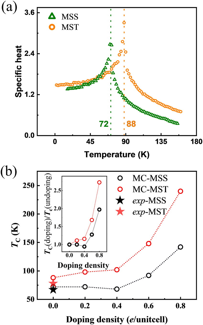
Based on this premise, by using eqn (10) and the magnetic exchange parameters for different concentrations of electron doping, we obtained the trend of TC, as shown in Fig. S3 (ESI†). The TC of both MSS and MST first decreases slightly as the doping concentration increases. This is likely because, although the antiferromagnetic interaction given by J2 becomes smaller in magnitude, J1 and J3 likewise become smaller. As the doping concentration exceeds 0.4 e per unitcell, the TC rises significantly. This can be well explained by the change in sign of J2: indeed, the parallel configuration within the Mn1-hexagonal sublattice, already favoured by the strong AFM interaction Jinter between the Mn1 and Mn2 sublattices, is further stabilized by a ferromagnetic J2 interaction. As both J4 and J5 are found to weakly depend on doping, the TC enhancement can be understood essentially in the same way when considering the effective Jintra = J2 + 2J4 + J5. The results of the MF theory show that electron doping can raise the TC from 143 K to 200 K for MSS and from 185 K to 312 K for MST. Since MF is known to be not quantitatively reliable, MC simulations were performed for the J1–J5 model to confirm the above trends and conclusions. Before discussing the trends vs. electron doping, we show in Fig. 6(a) the specific heat of undoped MSS and MST as a function of temperature, the peak in the response function signalling the ordering temperature. It can therefore be easily deduced that the TC of undoped MSS and MST are 72 and 88 K, which are very close to the experimental values of 67 and 78 K, respectively.19,21 As shown in Fig. S4 (ESI†), where we determined TC from the peak of susceptibility, MC simulations vs. electron doping predict the same trend as that predicted by MF theory (cfr Fig. S3, ESI† and its inset figure): the TC increases from 72 to 142 K and 88 to 240 K for MSS and MST, respectively.
 |
| | Fig. 6 (a) Specific heat of MST (yellow circles) and MSS (green triangles) from MC simulations. (b) TC of MSS (black symbols) and MST (red symbols) as a function of doping concentration. The solid starts show the experimentally measured TC of MSS and MST without doping. The inset is the comparison of relative critical temperatures TC (doping)/TC (undoping) as a function of doping density. | |
5 Conclusions
In this work, we investigated the properties of the magnetically-frustrated ferrimagnetic materials MSS and MST using first principles calculations. In particular, we proposed electron doping as a working recipe to increase the Curie temperature. We quantitatively show that the magnetic frustration can be reduced by electronic doping, which for certain levels even changes the sign of J2 and can therefore strengthen the ferrimagnetic configuration. The higher TC brought about by electronic doping was confirmed by both MF theory and MC simulations. In addition, the electronic and magnetic properties of MSS and MST are discussed, finding that they are qualitatively similar, but not quantitatively the same. In particular, the two compounds do not respond in the same way to electronic doping. We have therefore discussed the mechanisms underlying the MSS and MST different responses in detail and interpreted the differences in terms of larger electronegativity and smaller SOC-strength of the anion and of different energy position of Mn states in MSS compared to MST.
Conflicts of interest
There are no conflicts to declare.
Acknowledgements
This work was supported by National Natural Science Foundation of China (grants no. 12074241, 11929401, 52130204, 12311530675), Science and Technology Commission of Shanghai Municipality (grants no. 22XD1400900, 22YF1413300, 20501130600, 21JC1402600, and 21JC1402700), High Performance Computing Center, Shanghai University, High Performance Computing Center, Shanghai Technical Service Center of Science and Engineering Computing. L. Q. acknowledges the support of China Scholarship Council. P. B. and S. P. acknowledge financial support from the Italian Ministry for Research and Education through PRIN-2017 projects Tuning and understanding Quantum phases in 2D materials—Quantum 2D (IT-MIUR grant no. 2017Z8TS5B) and ‘ToWards fErroElectricity in Two dimensions-TWEET’ (IT-MIUR grant no. 2017YCTB59), respectively. P. K. and S. P. acknowledge support from the Royal Society through the International Exchange grant IEC\R2\222041. PK acknowledges support from The Leverhulme Trust via grant no. RL-2016-006, and the UK Engineering and Physical Sciences Research Council via grant no. EP/X015556/1.
Notes and references
- A. F. May, Y. Liu, S. Calder, D. S. Parker, T. Pandey, E. Cakmak, H. Cao, J. Yan and M. A. McGuire, Phys. Rev. B, 2017, 95, 174440 CrossRef.
- A. F. May, H. Cao and S. Calder, J. Magn. Magn. Mater., 2020, 511, 166936 CrossRef CAS.
- J. Kanamori, J. Phys. Chem. Solids, 1959, 10, 87–98 CrossRef CAS.
- L. Martinez, C. Saiz, A. Cosio, R. Olmos, H. Iturriaga, L. Shao and S. Singamaneni, MRS Adv., 2019, 4, 2177–2184 CrossRef CAS.
- L. Martinez, H. Iturriaga, R. Olmos, L. Shao, Y. Liu, T. T. Mai, C. Petrovic, A. R. Hight Walker and S. Singamaneni, Appl. Phys. Lett., 2020, 116, 172404 CrossRef CAS.
- Y. Liu, Z. Hu, M. Abeykoon, E. Stavitski, K. Attenkofer, E. D. Bauer and C. Petrovic,
et al.
, Phys. Rev. B, 2021, 103, 245122 CrossRef CAS.
- Y. Zhang, L.-F. Lin, A. Moreo and E. Dagotto, Phys. Rev. B, 2023, 107, 054430 CrossRef CAS.
- Y. Ni, H. Zhao, Y. Zhang, B. Hu, I. Kimchi and G. Cao, Phys. Rev. B, 2021, 103, L161105 CrossRef CAS.
- G. Sala, J. Lin, A. Samarakoon, D. Parker, A. May and M. Stone, Phys. Rev. B, 2022, 105, 214405 CrossRef CAS.
- J. Wang, S. Wang, X. He, Y. Zhou, C. An, M. Zhang, Y. Zhou, Y. Han, X. Chen and J. Zhou,
et al.
, Phys. Rev. B, 2022, 106, 045106 CrossRef CAS.
- J. Seo, C. De, H. Ha, J. E. Lee, S. Park, J. Park, Y. Skourski, E. S. Choi, B. Kim and G. Y. Cho,
et al.
, Nature, 2021, 599, 576–581 CrossRef CAS PubMed.
- Y. Liu and C. Petrovic,
et al.
, Phys. Rev. B, 2018, 98, 064423 CrossRef CAS.
- R. Olmos, J. A. Delgado, H. Iturriaga, L. M. Martinez, C. L. Saiz, L. Shao, Y. Liu, C. Petrovic and S. R. Singamaneni, J. Appl. Phys., 2021, 130, 013902 CrossRef CAS.
- F. Ye, M. Matsuda, Z. Morgan, T. Sherline, Y. Ni, H. Zhao and G. Cao, Phys. Rev. B, 2022, 106, L180402 CrossRef CAS.
- S. Xu, F. Jia, X. Yu, S. Hu, H. Gao and W. Ren, Mater. Today Phys., 2022, 27, 100775 CrossRef CAS.
- E. S. Morell, A. León, R. H. Miwa and P. Vargas, 2D Mater., 2019, 6, 025020 CrossRef CAS.
- C. Gong, L. Li, Z. Li, H. Ji, A. Stern, Y. Xia, T. Cao, W. Bao, C. Wang and Y. Wang,
et al.
, Nature, 2017, 546, 265–269 CrossRef CAS PubMed.
- M. Yang, Q. Li, R. V. Chopdekar, C. Stan, S. Cabrini, J. W. Choi, S. Wang, T. Wang, N. Gao and A. Scholl,
et al.
, Adv. Quantum Technol., 2020, 3, 2070041 CrossRef.
- X.-J. Dong, J.-Y. You, B. Gu and G. Su, Phys. Rev. Appl., 2019, 12, 014020 CrossRef CAS.
- M. Lu, Q. Yao, Q. Li, C. Xiao, C. Huang and E. Kan, J. Phys. Chem. C, 2020, 124, 22143–22149 CrossRef CAS.
- J. He, G. Ding, C. Zhong, S. Li, D. Li and G. Zhang, J. Mater. Chem. C, 2019, 7, 5084–5093 RSC.
- K. Wang, K. Ren, Y. Cheng, M. Zhang, H. Wang and G. Zhang, Phys. Chem. Chem. Phys., 2020, 22, 22047–22054 RSC.
- C. Song, W. Xiao, L. Li, Y. Lu, P. Jiang, C. Li, A. Chen and Z. Zhong, Phys. Rev. B, 2019, 99, 214435 CrossRef CAS.
- N. Liu, S. Zhou and J. Zhao, Phys. Rev. Mater., 2020, 4, 094003 CrossRef CAS.
- L. Zhang, X. Huang, H. Dai, M. Wang, H. Cheng, L. Tong, Z. Li, X. Han, X. Wang and L. Ye,
et al.
, Adv. Mater., 2020, 32, 2002032 CrossRef CAS PubMed.
- M. Mogi, A. Tsukazaki, Y. Kaneko, R. Yoshimi, K. Takahashi, M. Kawasaki and Y. Tokura, APL Mater., 2018, 6, 091104 CrossRef.
- L. Zhang, L. Song, H. Dai, J.-H. Yuan, M. Wang, X. Huang, L. Qiao, H. Cheng, X. Wang and W. Ren,
et al.
, Appl. Phys. Lett., 2020, 116, 042402 CrossRef CAS.
- C. Bigi, L. Qiao, C. Liu, P. Barone, M. C. Hatnean, G.-R. Siemann, B. Achinuq, D. A. Mayoh, G. Vinai and V. Polewczyk,
et al.
, Phys. Rev. B, 2023, 108, 054419, DOI:10.1103/PhysRevB.108.054419.
- J. P. Perdew, K. Burke and M. Ernzerhof, Phys. Rev. Lett., 1996, 77, 3865 CrossRef CAS PubMed.
- G. Kresse and J. Hafner, Phys. Rev. B: Condens. Matter Mater. Phys., 1993, 47, 558 CrossRef CAS PubMed.
- V. I. Anisimov, J. Zaanen and O. K. Andersen, Phys. Rev. B: Condens. Matter Mater. Phys., 1991, 44, 943 CrossRef CAS PubMed.
- P. E. Blöchl, O. Jepsen and O. K. Andersen, Phys. Rev. B: Condens. Matter Mater. Phys., 1994, 49, 16223 CrossRef PubMed.
- G. Kresse and D. Joubert, Phys. Rev. B: Condens. Matter Mater. Phys., 1999, 59, 1758 CrossRef CAS.
- H. J. Monkhorst and J. D. Pack, Phys. Rev. B: Solid State, 1976, 13, 5188 CrossRef.
- H. Xiang, C. Lee, H.-J. Koo, X. Gong and M.-H. Whangbo, Dalton Trans., 2013, 42, 823–853 RSC.
- R. F. Evans, W. J. Fan, P. Chureemart, T. A. Ostler, M. O. Ellis and R. W. Chantrell, J. Phys.: Condens. Matter, 2014, 26, 103202 CrossRef CAS PubMed.
- P. Asselin, R. F. L. Evans, J. Barker, R. W. Chantrell, R. Yanes, O. Chubykalo-Fesenko, D. Hinzke and U. Nowak, Phys. Rev. B: Condens. Matter Mater. Phys., 2010, 82, 054415 CrossRef.
- J. M. Crowley, J. Tahir-Kheli and W. A. Goddard III, J. Phys. Chem. Lett., 2016, 7, 1198–1203 CrossRef CAS PubMed.
- W.-B. Zhang, Q. Qu, P. Zhu and C.-H. Lam, J. Mater. Chem. C, 2015, 3, 12457–12468 RSC.
- Q. Song, C. A. Occhialini, E. Ergeçen, B. Ilyas, D. Amoroso, P. Barone, J. Kapeghian, K. Watanabe, T. Taniguchi and A. S. Botana,
et al.
, Nature, 2022, 602, 601–605 CrossRef CAS PubMed.
- Z. An, Y. Su, S. Ni and Z. Guan, J. Phys. Chem. C, 2022, 126, 11330–11340 CrossRef CAS.
|
| This journal is © the Owner Societies 2024 |
Click here to see how this site uses Cookies. View our privacy policy here. 
 ab,
Paolo
Barone
c,
Baishun
Yang
b,
Phil D.C.
King
d,
Wei
Ren
ab,
Paolo
Barone
c,
Baishun
Yang
b,
Phil D.C.
King
d,
Wei
Ren


 and
and  can be obtained: