Green–Kubo expressions for transport coefficients from dissipative particle dynamics simulations revisited
Received
8th August 2023
, Accepted 19th November 2023
First published on 1st December 2023
Abstract
This article addresses the debate about the correct application of Green–Kubo expressions for transport coefficients from dissipative particle dynamics simulations. We demonstrate that the Green–Kubo expressions are valid provided that (i) the dynamic model conserves the physical property, whose transport is studied, and (ii) the fluctuations satisfy detailed balance. As a result, the traditional expressions used in molecular dynamics can also be applied to dissipative particle dynamics simulations. However, taking the calculation of the shear viscosity as a paradigmatic example, a random contribution, whose strength scales as 1/δt1/2, with δt the time-step, can cause difficulties if the stress tensor is not separated into the different contributions. We compare our expression to that of Ernst and Brito (M. H. Ernst and R. Brito, Europhys. Lett., 2006, 73, 183–189), which arises from a diametrically different perspective. We demonstrate that the two expressions are completely equivalent and find exactly the same result both analytically and numerically. We show that the differences are not due to the lack of time-reversibility but instead from a pre-averaging of the random contributions. Despite the overall validity of Green–Kubo expressions, we find that the Einstein–Helfand relations (D. C. Malaspina et al. Phys. Chem. Chem. Phys., 2023, 25, 12025–12040) do not suffer from the need to decompose the stress tensor and can readily be used with a high degree of accuracy. Consequently, Einstein–Helfand relations should be seen as the preferred method to calculate transport coefficients from dissipative particle dynamics simulations.
1 Introduction
Green–Kubo (GK) and Einstein–Helfand (EH) formulas1,2 have been widely used to calculate the macroscopic transport coefficients of molecular systems from molecular dynamics simulations. Their use allows transport properties such as diffusion coefficients, shear viscosities, or thermal conductivities, to be obtained from the dynamics of the microscopic constituents simulated by a computer. Transport coefficients are defined from phenomenological relations between property fluxes and the so-called thermodynamic forces, related to gradients of state properties. An example is the thermal conductivity, λ, defined from Fourier's law as,where Jq is the heat flux density and T is the system temperature. Non-equilibrium simulations reproduce the experimental setup in which external gradients (e.g., temperature) are established giving rise to conjugate fluxes (e.g., heat) or conversely, fluxes are imposed that result in a conjugate gradient.3–5 Assuming a linear response, the associated transport coefficient is then obtained from the ratio λ ≃ Jxq/(dT/dx), if the gradient is in the x-direction. In contrast, equilibrium methods, such as GK and EH, rely on the measurement of the decay of the spontaneous thermal fluctuations of the corresponding physical property, and they do not require any special simulation setup to create the externally imposed gradients. As a consequence, a single equilibrium simulation with periodic boundary conditions can provide a plethora of transport coefficients for different properties as commonly found in molecular dynamics codes (e.g. LAMMPS6). Another advantage of equilibrium methods is found in simulations of microstructured systems, such as micellar suspensions, in which non-equilibrium methods can substantially deform these microstructures, even at very small gradients.
Despite the fact that GK and EH expressions are commonly used for Hamiltonian systems, doubts have been cast on their straightforward application to systems with dissipative and random forces. Dissipative Particle Dynamics (DPD) methods7–9 lie in this category, together with its extensions. These include many-body potentials (MB-DPD),10–12 energy-conserving DPD (DPDE)13,14 and variations that include different ensembles,.15–18 In ref. 19 a dependence of the DPD parameters on the overall system temperature has been introduced. More recently, a thermodynamically consistent method with density- and temperature-dependent potentials (GenDPDE), which are defined on particle state variables only, has been presented.20,21 Within GenDPDE, temperature-dependent strong non-equilibrium processes can be simulated.22 A more complete list of DPD methods can be found in several reviews.23–25 Due to the aforementioned theoretical concerns, different attempts to obtain what was thought to be the appropriate expressions for GK formulas appeared in the literature.26,27 These expressions differ from the standard GK formulas used for conservative systems and required further testing against non-equilibrium simulations to assess their validity. In ref. 28, such a comparative analysis is conducted for shear and bulk viscosities. According to those numerical calculations, the expression due to Ernst and Brito (EB)27 is the only formula that accurately reproduces the non-equilibrium results. However, the EB expression may look exotic for common practitioners of molecular dynamic simulations of conservative systems. On the one hand, the random contribution is not explicitly present, although one would intuitively expect that all forces should contribute to the total value of the viscosity. On the other hand, the signs of the various contributions involving the dissipative terms differ from the usual ones. Such an unusual structure of the EB formula hinders its generalisation to properties other than the shear and bulk viscosity, and may lead to inaccurate EH expressions29 when taken as the starting point.
In a previous article,30 nevertheless, we demonstrated the validity of the standard EH relations for all the DPD methods mentioned above, including the EH formula for the shear viscosity, which we have chosen as a benchmark for the discussion in this article. We proved that if the appropriate expression of the stress tensor for the model under study is derived, the EH formula can be straightforwardly applied. After an extensive simulation analysis, we verified that the standard EH relations provided shear viscosities as well as thermal conductivities in excellent agreement with the non-equilibrium simulations. Our theoretical approach is based on only two conditions that need to be satisfied by the dynamic algorithm. Namely, (i) the models preserve the conservation of the physical property whose transport is studied (e.g., particle number, momentum or energy, among others), and (ii) the transition probabilities generated by the dynamic algorithm satisfy Detailed Balance (DB). It is well known that DB stems precisely from the time-reversibility of the microscopic equations of motion (EoM), but no time-reversibility of the actual DPD trajectories is needed to derive the suitable EH expressions.
In this article, we extend our analysis to the GK formulas as they can be directly compared to the EB expressions. We demonstrate that the standard expressions for the GK formulas are in fact valid for DPD algorithms if the appropriate forms of the mesoscopic property fluxes (the stress tensor for the case considered) are used. These forms are exactly the same as those derived for the EH formulas in ref. 30. Moreover, we also demonstrate that remarkably our more physically intuitive formulation of the GK formulas can be cast under the EB form, proving the exact equivalence between both formulas, which is the main result of this article. While the standard expressions that include dissipative and random terms have already been successfully applied for DPD methods,31,32 we believe that the main reason this straightforward procedure has not been more frequently used is the difficulty in obtaining statistically significant data with a reasonable simulation time, as demonstrated below.
In the following section, a general derivation of the GK expressions for transport coefficients is given. This is followed by a summary of the standard DPD algorithm and the derivation of the corresponding GK expression for the shear viscosity. In the Simulation methods section, we give the details of both, the equilibrium and non-equilibrium simulations, including all of the parameters employed. We then present the results of our simulations and provide a detailed analysis of the different contributions to the stress tensor. We show that the EB expression is equivalent to ours, despite their formal differences. Finally, we highlight the advantages of EH over GK expressions and argue why the former should be preferred when calculating transport properties. We end the article with the main conclusions from our work.
2 Theoretical analysis
DPD algorithms are categorised as mesoscopic methods since they describe the dynamics of a collection of resolved degrees of freedom (DoF), singled out from the total number of DoF of a given underlying physical system. Hence, dissipative as well as random interactions arise due to the coupling of the resolved DoFs with the unresolved (coarse-grained) DoFs. However, the physical properties of these mesoscopic models are inherited from the Hamiltonian microscopic system, whose dynamics is time-reversible. Consequences of this fact are first, that an equilibrium probability distribution for the resolved DoF can be defined, and second, that the transition probabilities induced by the dynamic algorithm need to satisfy DB when in thermal equilibrium.
2.1 General derivation of Green–Kubo expressions
To derive the GK relation for a given transport coefficient, let us first consider that the DPD algorithm conserves a given property a transported by the mesoparticles. Examples of property conservation include the number of particles in Langevin equations to study Brownian motion, particle number and momentum in standard DPD, together with the extension to include the energy in DPDE, among others. Due to this dynamic conservation of a, a macroscopic conserved field A exists, and is given as| |  | (2) |
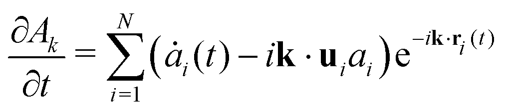
where r is a field point and ri(t) is the position of the mesoparticle i at time t. We also introduce Fourier's representation of A as| |  | (3) |
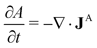
where k is the wavevector. Hence, A satisfies the balance equation| |  | (4) |
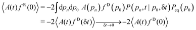
where JA is the flux density of A. Since a is conserved, 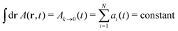 . Eqn (4) is not a closed equation as long as JA remains undefined. Phenomenological equations, analogous to eqn (1) for the energy transport, are required to provide a closure that will produce a well posed equation for the evolution of A. In the framework of Onsager's theory of linear irreversible thermodynamics,33,34 the closure is given in the form of a linear relation between the flux and the thermodynamic forces. For the simple case analysed here as a proof of concept, we consider that the thermodynamic force can be written as a gradient of A, in analogy with Fourier's law for the heat transport or Newton's law for the shear viscosity.† Hence, the flux density becomes,Advective contributions expressed as vA (v is the velocity field) are neglected in eqn (5) as they are outside the linear response theory. The first term on the right-hand side of eqn (5) introduces the transport coefficient α that needs to be determined. This term contains the dissipative effects leading to the decay of the perturbations in A. The second term contains the effect of the thermal fluctuations, which arise from the interaction between the macroscopic and mesoscopic behaviour alongside with the dissipation. Here, for simplicity, we have only considered a single field with no coupling with other fields, in contrast to, e.g., the Ludwig–Soret effect34 (see ref. 35 for more details).
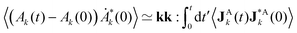
Therefore, the relaxation of the fluctuations of Ak in thermal equilibrium satisfies
| |  | (6) |
where from
eqn (5), we get
| | | −ik·JAk = −αk2Ak − ik·JA,Rk | (7) |
Alternatively, from
eqn (3), we can also write the balance equation in terms of the mesoscopic variables as
| |  | (8) |
where
ui =
ṙi. Since the stochastic algorithm is formulated in discrete form, we have to interpret
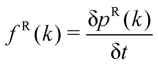
ui = (
ri(
t + δ
t) −
ri(
t))/δ
t with no loss of generality. As a consequence, a dependence on the timestep δ
t is possible as the trajectories generated depend on it. In addition, if
a is exchanged between mesoparticles, which occurs when
a is the energy content of the particle in DPDE, then an additional dynamics for the evolution of
a is necessary. Thus, it is crucial to realise that
eqn (6) with
eqn (7), is actually the same as
eqn (8).
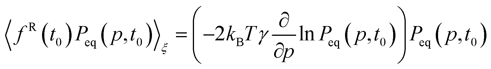
Following the derivation in ref. 30, the properties of JA,Rk are determined by DB. On the one hand, we obtain
while, on the other hand, the corresponding Fluctuation–Dissipation Theorem (FDT) is
| |  | (10) |
In
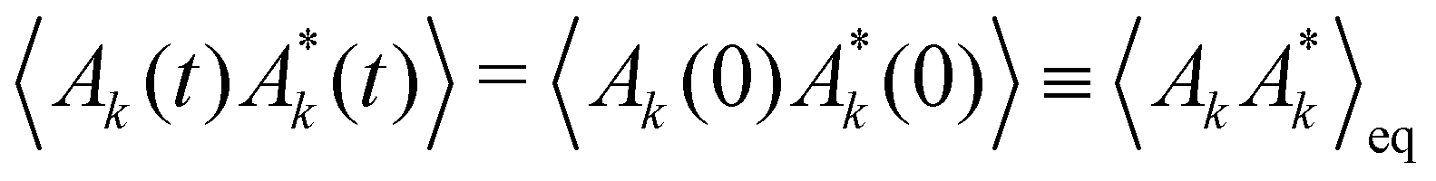
eqn (10), the superscript * denotes the complex-conjugate, which is needed to enforce spatial translational invariance of the correlation function. Moreover, the equilibrium equal-time correlation function is time-translational invariant and hence,
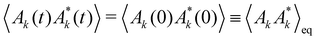
.
We start by deriving the formal solution of eqn (6) with eqn (7):
| |  | (11) |
Next, we consider the correlation function

in terms of the dynamics of the fields,
i.e.,
| |  | (12) |
First, from
eqn (12) one needs to realise that odd terms in
JA,Rk vanish by symmetry. Moreover in the hydrodynamic limit,
k2t → 0 and thus,

. As a consequence, the product of the initial conditions is

and can be neglected. Therefore, the leading contribution in the hydrodynamic limit becomes,
| | 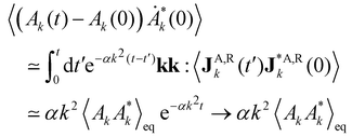 | (13) |
which is

. In deriving the last equality, we used
eqn (10). In addition, we considered that the integration of the correlation

over time with
t′ ≥ 0 introduces a factor of 1/2 due to causality applied on the even Dirac's δ-function.
36 Using
eqn (6) for
Ȧk(0) and the formal solution,
eqn (11), with
k2t → 0, we get
| |  | (14) |
and therefore
| | 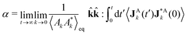 | (15) |
which is the standard form of the GK expressions.
2.2 Standard DPD algorithm
In this section, we summarise the standard DPD algorithm7,8 as we use only this method in the subsequent discussion of our theoretical approach. Pairwise, many-body or any other type of potential forces are included because our results are independent of their explicit form. Furthermore, the analysis of the stress tensor used for demonstration in this work also applies to DPDE methods,13,14,37,38 as well as to GenDPDE methods,20,21 and their variants, including the inter-particle mass transfer (GenDPDE-M),39,40 since the dynamics of the momentum is represented by the same equation and is independent of other properties exchanged by the mesoparticles.
DPD is a particulate Lagrangian method developed to simulate hydrodynamic behaviour at the mesoscopic level. The particle–particle interaction satisfies particle-number conservation, as in Brownian dynamics, but additionally momentum is also conserved. The latter guarantees hydrodynamic behaviour of the resulting velocity field at long wavelengths and long times, and therefore, the existence of a Navier–Stokes equation with the corresponding viscosity coefficients. Fig. 1 outlines the relevant variables present in DPD.
 |
| | Fig. 1 Schematic of the DPD simulation method governed by EoM (16) and (17). | |
The dynamics of the mechanical DoF, i.e., particle positions, ri, and momenta, pi, is given by the following EoM:
| |  | (16) |
| |  | (17) |
where prime and non-prime variables refer to times
t + δ
t and
t, respectively,
mi is the mass of mesoparticle
i,
fCi and
fDi are the conservative and dissipative forces, respectively, and δ
pRij is the random contribution to the momentum, proportional to a Wiener process, exchanged between particles
i and
j. Therefore, the
random force is given by
| |  | (18) |
For the dissipative force, we consider the traditional pairwise additive form
| | 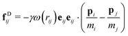 | (19) |
where
γ is the friction coefficient and
ω(
rij) is the weighting function, which is a smooth positive-definite function of the interparticle distance with a cut-off range
rc. The random contribution to the momentum, δ
pRij, satisfies the FDT
8| |  | (20) |
where δ
pRij = −δ
pRji,
kB is the Boltzmann constant,
eij = (
ri −
rj)/|
ri −
rj|, and
T is the system temperature, considered to be fixed by an external reservoir. The normalised Gaussian random numbers
ξij satisfy
| |  | (22) |
where the average is taken over the probability distribution of
ξij and
δij is the Kronecker delta symbol, which is 1 if
i =
j and 0 otherwise. Note that here
δtt′ is 1 if
t and
t′ are inside the same time interval of width δ
t, and zero otherwise.
2.3 Green–Kubo formula for the shear viscosity in DPD methods
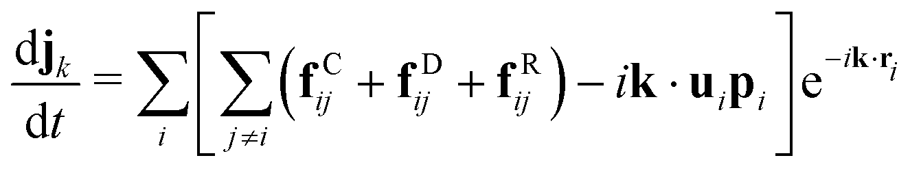
The derivation of the mesoscopic form of the stress tensor requires the analysis of the dynamics of the momentum density, represented here by the observable,| |  | (23) |
From eqn (8) in discrete form, we evaluate the time-derivative of the observable as| |  | (24) |
Note that, in view of eqn (6), the term −ik·uipi in eqn (24) already has the form of a divergence of a flux in the Fourier space. However, the term involving the forces needs further development. Effectively, introducing fij ≡ fCij + fDij + fRij, to simplify the notation, we can write,| |  | (25) |
The order of summation in the last term on the right-hand side of eqn (25) can be inverted to get,| |  | (26) |
Then, we exchange i ↔ j in the last term on the right-hand side of eqn (26) and use fji = −fij to obtain| |  | (27) |
Since the interaction range for all the forces is limited to rc, k·rji ≪ 1 in the long-wavelength limit, and the second exponential in eqn (27) can be expanded to the lowest non-zero order to get,| |  | (28) |
After gathering all the contributions, we obtain,| |  | (29) |
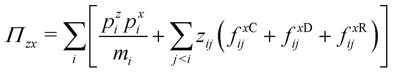
To study shear waves, the velocity field needs to be orthogonal to the wavevector ![[k with combining circumflex]](https://www.rsc.org/images/entities/b_char_006b_0302.gif) . We thus arbitrarily choose the x-component of the momentum, the z-component of k in eqn (29), and obtain
. We thus arbitrarily choose the x-component of the momentum, the z-component of k in eqn (29), and obtain| | 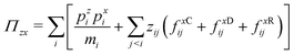 | (30) |
In eqn (30), we observe that both, the dissipative and random forces, should be incorporated in the calculation of the correlation since they contribute to the global momentum balance, along with the conservative forces. However, it is very important to realise that while fCi and fDi depend only on the state variables of the system ri and pi, fRij also depends on timestep δt since  (see eqn (18) and (20)). Hence, unlike in conservative systems, DPD trajectories strongly depend on the size of δt.
Following the same approach as in ref. 30, we recall that the linearised Navier–Stokes equation for the x-component at the macroscopic level is
| |  | (31) |
Comparing
eqn (31) with
eqn (6), using
eqn (7), and taking into account that here
Ak(
t) ≡
jk(
t),
cf.eqn (23), then it follows that
α ≡
ν =
η/
ρ. Moreover, since
, from
eqn (15) we finally obtain,
| |  | (32) |
which is the traditional GK expression for the shear viscosity found in the literature.
35 Hence, we can conclude that (i) the traditional GK formula is valid for the DPD algorithm, and (ii) the stress tensor must contain all of the DPD forces, including the dissipative and random ones.
3 Simulation methods
3.1 Equilibrium simulation details
We used our in-house DPD code with a velocity-Verlet integration scheme, which is implemented in Fortran with OpenMP parallelisation (see e.g. ref. 41 for further discussion on DPD integration algorithms). All simulations were performed in reduced units, where rc is the unit of length, m is the unit of mass, and kBT is the unit of energy. Therefore, the unit of time becomes  . The DPD systems contained N = 20
![[thin space (1/6-em)]](https://www.rsc.org/images/entities/char_2009.gif) 000 mesoparticles in a volume V and the simulation box was cubic with periodic boundary conditions in all three directions. Values of V were changed in each simulation to obtain the required system particle densities,
000 mesoparticles in a volume V and the simulation box was cubic with periodic boundary conditions in all three directions. Values of V were changed in each simulation to obtain the required system particle densities, ![[n with combining macron]](https://www.rsc.org/images/entities/i_char_006e_0304.gif) = N/V. In Table 1, we summarise the parameters employed in the simulations.
= N/V. In Table 1, we summarise the parameters employed in the simulations.
Table 1 Equilibrium simulation parameters for the calculation of the viscosity by the GK formula, eqn (32); is the system particle number density, γ is the dissipative coefficient, and δt is the timestep
| System |
|
γ
|
δt |
Samples (×103) |
| 1 |
3 |
5 |
0.01 |
500 |
| 1b |
3 |
5 |
0.001 |
500 |
| 2 |
4 |
5 |
0.01 |
500 |
| 3 |
5 |
5 |
0.01 |
500 |
| 4 |
6 |
5 |
0.01 |
500 |
| 5 |
7 |
5 |
0.01 |
500 |
| 6 |
8 |
5 |
0.005 |
500 |
| 7 |
16 |
5 |
0.002 |
5 |
| 8 |
32 |
5 |
0.001 |
5 |
In all of the simulations, the weighting function is given by
| |  | (33) |
where
ω(
r) = 0 for
r >
rc. To directly compare our simulations with shear viscosity data existing in the literature, we did not consider conservative forces between mesoparticles,
i.e., only dissipative and random forces were considered. However, no conceptual limitation exists regarding the addition of conservative forces when the GK expression
eqn (32) is employed.
The conditions of systems 1, 2, 3, 4, and 5 in Table 1 correspond to the ones in ref. 28. The length τs of the time-series Πzx(t), used as samples in the relevant averages of the correlation functions, was τs = 20, 15, 10, 8, and 5 for = 3, 4, 5, 6, and 7, respectively. A new sample was created from the system's trajectory every 20 timesteps with a total simulation length of 107 timesteps. For completion, we have also performed simulations for higher densities = 8, 16, and 32, which correspond to systems 6, 7, and 8 in Table 1.
3.2 Viscosity obtained from non-equilibrium simulations
To test the validity of the GK expression eqn (32), with the stress tensor given in eqn (30), we calculated the viscosity independently from a series of non-equilibrium DPD simulations. For the latter, the box length in the x-direction, Lx, was twice as large as in the other two directions, i.e., Ly = Lz = Lx/2, and periodic boundary conditions were applied in all directions. The shear rate was induced using a modified PeX method,4,5 in which we defined two narrow slabs of width Δx = Lx/10, in specific locations along the x-axis. Then, at a given rate, we exchanged the largest momentum in the positive z-direction of a mesoparticle within the slab located at x = Lx/4, with the momentum of the particle with the largest momentum in the negative z-direction of the slab located at x = 3Lx/4. The timestep for the simulations is the same as in the corresponding equilibrium simulations as given in Table 1. The viscosity η by the PeX method follows from the constitutive equation,| |  | (34) |
where dvz/dx is the induced velocity gradient between the slabs, and Πxz is the shear stress imposed due to the momentum exchange between slabs. On the one hand, we measured the actual shear rate from a linear regression of the velocity profile in the central region of the system (see Fig. 2). On the other hand, Πxz is obtained as,| |  | (35) |
where Δpz is the accumulated momentum exchanged between the slabs in a sufficiently long time-interval Δt, starting after the system reaches steady state, nexc is the frequency of the momenta exchange, which is the effective control parameter of Πxz, and LzLy is the cross-sectional area of the x-side of the box.
 |
| | Fig. 2 Average velocity profile for a DPD system at the system number density 3 (red line). The profile is obtained from velocities in z-direction vs. positions in the x-direction in the non-equilibrium simulation set-up. From this data, a linear regression is applied in the central part of the simulation box (dashed black line) to obtain the corresponding value of dvz/dx in eqn (34). | |
4 Results and discussion
4.1 Application of the standard Green–Kubo formula
The direct application of the standard GK approach, eqn (32), to the stochastic trajectories is possible and it gives the correct values of the transport coefficients. In Fig. 3a, we show the stress-correlation function C(t) = 〈Πzx(t)Πzx(0)〉 for System 1, cf.Table 1. To obtain a reliable (independent of arbitrary choices) estimate of C(t)'s time-integral, due to the presence of a spike at t = 0, we proceeded by numerically integrating the first few s timesteps using the trapezoidal rule. The remaining correlation for C(t > sδt) was fitted to a stretched exponential of the form,| | Cfit(t) = B![[thin space (1/6-em)]](https://www.rsc.org/images/entities/i_char_2009.gif) exp(−ctd) exp(−ctd) | (36) |
able to capture the hydrodynamic behaviour and tending to zero at long time. The parameters B, c and d are positive constants, and the error was calculated from the error in the integral due to the calculated uncertainties in fitting these parameters. Since the stretched exponential tends to zero at t → ∞, the numerical integration of the fit Cfit(t) produces an accurate prediction of the time-integral. Our results are independent of the choice of s and the total length of the correlation, provided that the final time was sufficiently large such that the fitted function decayed to zero. After choosing s = 2, the obtained estimate of the viscosity using the standard GK formula eqn (32), η = 1.28 ± 0.01, is in very good agreement with the non-equilibrium value, ηne = 1.2773. We observed that the main difficulty in obtaining the value of η from the stress tensor correlation data is the dispersion of the values as shown in Fig. 3a. This is due to the effect of the random components of the stress tensor ΠRzx for a given number of sample trajectories, which give rise to the spike at the first timestep, but is also responsible for the dispersion of the data at longer times. The EB formula, with no explicit contribution of ΠRzx, provides a narrower confidence range. To illustrate the inherent difficulty in obtaining reliable numerical estimates of the viscosity from the direct application of the GK formula eqn (32), we show in Fig. 3b the same correlation function as for System 1, but with a ten times smaller δt = 0.001, referred to as System 1b. In this case, the dispersion of the data significantly increased for the same number of sample trajectories yielding a less reliable numerical analysis. For a comparison with System 1 for the same time-range, we set the numerical integration of the initial steps to s = 20, since the timestep was reduced by a factor of 10. Despite the dispersion in the data, the numerical fit still provides a reasonable value of η, although with a much lower precision, i.e., η = 1.36 ± 0.09. Despite the intrinsic difficulties associated with the straighforward application of the GK formula (32), there are studies for low-density DPD systems reporting accurate results for η.31,32 However, when the dissipative interactions increase and the timestep is reduced, to correctly integrate the EoM of DPD, the GK approach may become unreliable.
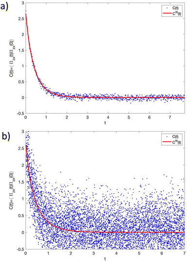 |
| | Fig. 3 Stress tensor correlation as a function of time along with the regression curve eqn (36). (a) System 1: decay of the correlation C(t > sδt) for s = 2. The value of the viscosity obtained from the GK expression eqn (32) is η = 1.28 ± 0.01 which can be compared to η = 1.2773 obtained from non-equilibrium simulations. (b) System 1b: decay of the correlation C(t > sδt) for s = 20, so that the regression curve covers the same time span as for the System 1, but with a timestep ten times smaller. Despite the large dispersion, a reasonable value of η = 1.36 ± 0.09 was still obtained. | |
Therefore, considerable computational effort may be required to obtain reliable results under certain conditions. While this is not a conceptual flaw in the application of the standard GK expression to DPD algorithms, the equivalent EH formula does not suffer from such drawbacks, and should be the preferred method in this case.
4.2 Analysis of the different contributions to the stress tensor and comparison with the EB formula.
According to eqn (30), the stress tensor can be separated into three terms, based on the conservative, dissipative and random interactions as,| |  | (37) |
each defined by the corresponding term between brackets on the right-hand side of this equation. Note that we gathered the kinetic and conservative-force terms into the conservative contribution to the stress tensor, ΠCzx.
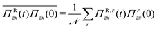
When these stress-tensor contributions are inserted into the correlation function, 〈Πzx(t)Πzx(0)〉, the decomposition leads to nine different contributions. Rather than separately analysing each contribution, we focus only on the aspects that are relevant for the objectives of this work. First, one should realise that 〈ΠRzx(t)ΠRzx(0)〉 is by construction only non-zero at the first time step, which allows one to calculate the correlation analytically as
| |  | (38) |
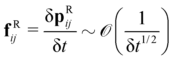
Note that the magnitude of this contribution is proportional to 1/δ
t as a result of the fact that the strength of the random force depends on 1/δ
t1/2,
cf.eqn (18). This fact may be surprising since it is not present in simulations of purely conservative systems, where the use of GK formulas is extensive. Moreover, such a dependence on the timestep may be concealed if a continuum time is considered.
The time integration of eqn (38) using the trapezoidal rule gives a constant value and naturally introduces a factor of 1/2 compatible with the integration of half the Dirac's δ(t) due to causality,36 as discussed after eqn (13). This constant contribution to η was already identified by Ernst and Brito27 and denoted as η∞. For our model, it is expressed as,
| |  | (39) |
It is important to realise that, although the correlation in
eqn (38) depends on the time-step, its contribution to the viscosity coefficient
eqn (39) is independent, as it corresponds to a material property of a dynamic system that conserves momentum. Therefore, although the choice of the size of the time-step affects the trajectories of the system, its statistical properties are not affected, due to the FD, and the overall hydrodynamic behaviour is insensitive to δ
t, provided that it is kept sufficiently small. From a numerical point of view, the dispersion in the data observed in
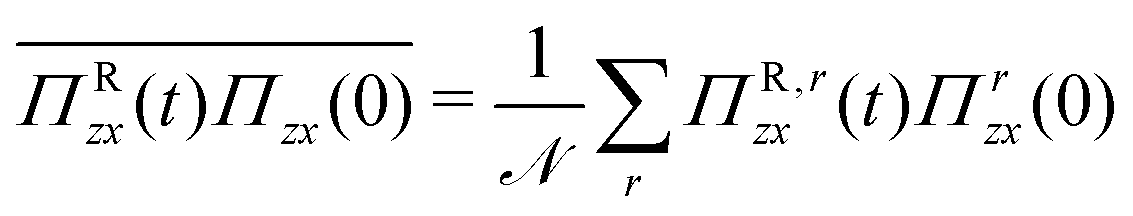
Fig. 3 is caused by the contribution 〈
ΠRzx(
t)
Πzx(0)〉, which averages to zero after the first timestep. However, in the straightforward application of the GK formula, such a correlation is numerically estimated as a mean over a finite number of samples
r = 1,…,
![[scr N, script letter N]](https://www.rsc.org/images/entities/char_e52d.gif)
,
i.e., as
, where
ΠR,rzx(
t)
Πrzx is the value of the product along one particular system trajectory
r. Then according to elementary statistical inference theory
| |  | (40) |
where
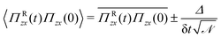
Δ is given in terms of constant parameters of the system and can be estimated as
Δ ∼
kBTγrc2N2/
V, from
eqn (38). Therefore, the direct use of
eqn (15) to obtain
η is affected by an uncertainty that
depends on the timestep as 1/δ
t for a correlation that could actually be set to zero except at the first timestep. For further illustration, consider a DPD simulation with δ
t involving

samples, and then another DPD simulation with a smaller timestep δ
t′ < δ
t. To have the same precision as in the former, the latter requires a larger number of samples,
i.e.
. This fact impairs a practical use of the standard formula
eqn (15) to obtain the viscosity, as the size of the sampling required may become computationally unaffordable. Therefore, although the viscosity coefficient for the DPD model exists and is well defined as an overall dynamic coefficient, independent of the time-step, its determination from the statistical methods underlying the Green–Kubo expression can be strongly impaired by data dispersion, which crucially depends upon the size of the time-step. Such inherent difficulty can be strongly reduced by singling out the contribution
eqn (39) from the rest of the correlation, which does not suffer from such statistical impairment.
So far we have shown that the direct application of the standard GK expression for DPD systems, although physically correct, may present statistical difficulties. Nevertheless, we continue with the objective of finding an expression that can be more tractable than eqn (32), with the stress tensor given in eqn (30). This can be done by first separating the contribution due to the first timestep, as given by eqn (39) and, second, by setting 〈ΠRzx(t)ΠC,Dzx(0)〉 = 0, since the random term is not correlated with the state of the system in the past, by construction. Then, eqn (32) becomes,
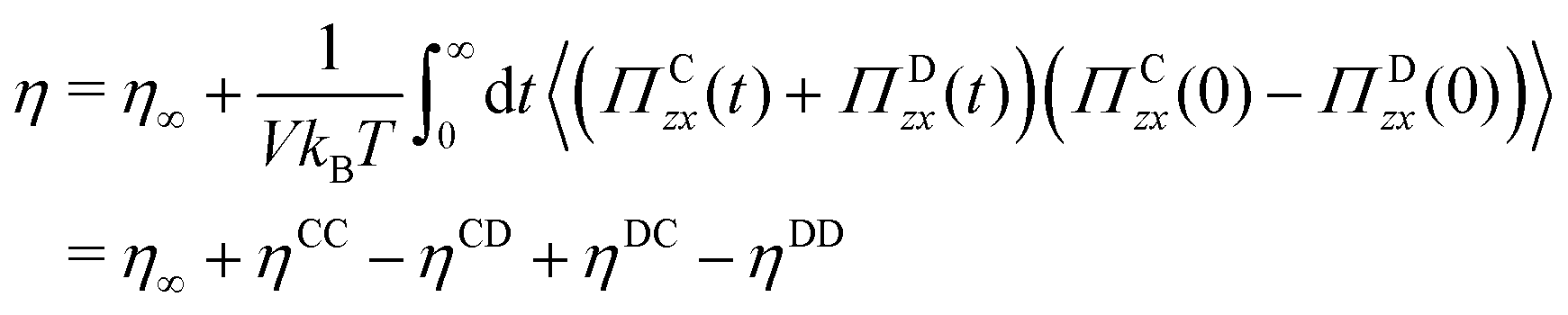
| | 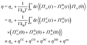 | (41) |
where

and
| |  | (42) |
This expression is in stark contrast with that given by Ernst and Brito in eqn (13) of ref. 27, which reads instead,
| |  | (43) |
However, although
eqn (41) and (43) may appear irreconcilable, they are actually the same due to the fact that, when averaging over the random terms,
ηres = −2(
ηCD +
ηDD), because
| | 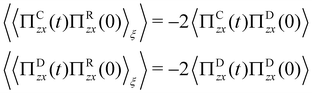 | (44) |
In
eqn (44), the inner averages 〈·〉
ξ on the left-hand side are included to emphasise that the equality occurs after averaging with respect to the random terms. In
Fig. 4, we numerically show that the correlation functions
C(
t) = 〈(
Πzx(
t) −
ΠRzx(
t))
Πzx(0)〉 and
CEB(
t) = 〈(
ΠCzx(
t) +
ΠDzx(
t))(
ΠCzx(0) −
ΠCzx(0))〉, whose time-integral yields
η −
η∞, are equal within simulation uncertainties. Additionally, in Appendix A we outline the derivation of the equalities
eqn (44). Moreover, we compared our results for
η with those obtained by non-equilibrium simulations
28 and the EB formula
eqn (43), and found excellent agreement, as can be seen in
Fig. 5.
 |
| | Fig. 4 Comparison between the correlation functions C(t) = 〈(Πzx(t) − ΠRzx(t))Πzx(0)〉 and CEB(t) = 〈(ΠCzx(t) + ΠDzx(t))(ΠCzx(0) − ΠDzx(0))〉 for System 5. | |
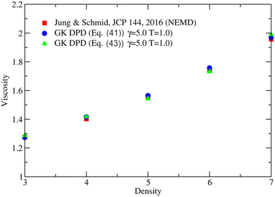 |
| | Fig. 5 Shear viscosity as a function of the system density comparing non-equilibrium simulations28 (red squares) with different GK expressions (blue dots are for the GK formula (41) while green triangles are for the GK formula (43)). Both GK shear viscosity values were calculated with our simulation data. The error bars are smaller than the size of the symbols. | |
Therefore, the equality
| |  | (45) |
is another important result of this work as it resolves the controversy regarding the use of the traditional GK formulas in DPD simulations due to the lack of time reversibility of stochastic trajectories. Hence, we conclude that, when the conditions of momentum conservation and DB are satisfied, mesoscopic systems with dissipative and random forces follow the same dynamic principles as conservative systems for determining transport coefficients. Therefore, difficulties associated with the use of the GK formulas are of a technical nature, and not due to any fundamental flaw in
eqn (32).
4.3 Preference for Einstein–Helfand over Green–Kubo formulas in DPD systems
In the previous subsection, we demonstrated that it is possible to use the standard GK formula eqn (32) in DPD simulations, although its use may be impractical. By extracting the zero-time correlation and eliminating the zero-average contributions involving the random stress tensor, we obtain a more practical GK formula eqn (41). We further demonstrated that the latter is equivalent to the EB formula eqn (43). However in both approaches, the tail contribution of the correlation functions needs to be fitted to a function that decays to zero. Otherwise, the value of the time-integral is sensitive to the final time chosen, due to the statistical fluctuations. The form of the fitting function has to be carefully chosen as the decay of the correlation functions may not be monotonous. The chosen form given in eqn (36) is monotonous and can only be used in sections of the correlation function with no change of sign in the derivative. For instance, for large densities such as in System 8, negative values of the correlation eqn (41) occur. In this case, we have used the same fitting function, but starting after the minimum of the correlation from which the decay is monotonous, and obtained again accurate results.
In contrast, in our previous article,30 we demonstrated that the EH expressions can be straightforwardly used to determine transport coefficients from DPD simulations. We found the traditional expression,
| |  | (46) |
where
Πzx is also given by
eqn (37) and includes both random and dissipative contributions. The application of the EH formula
eqn (46) is neither hampered by the statistical problems of the GK counterpart nor does it require any fitting function for the tail of the correlation. The standard procedure is to obtain the coefficient from a simple linear regression in the
diffusive regime. The reason for its superior statistical precision is due to the additional time-integral present in the EH formula. Effectively, interpreting the integration as a Riemann sum over the timesteps,
e.g. we get for the random contribution
ΠRzx| |  | (47) |
where
t =
kδ
t. According to
eqn (18) and (20), every element in the Riemann sum scales with the timestep as
and therefore, every element of the sum tends to zero as δ
t → 0. In contrast, in the standard GK formula the elements intervening in the correlation function are

. Therefore, their dispersion increased as δ
t decreased, causing the evaluation of the correlation to become more difficult (see
Fig. 3). The use of the EH formula requires no decomposition to reduce the statistical noise,
30 and there is no need for a specific combination of stress–tensor contributions to be introduced, which differs from the approach in ref.
27.
Since the EH formula eqn (46) follows from first principles, it can be used for any system provided that the flux of the conserved property (the stress tensor here) is properly derived from the dynamic algorithm. This derivation follows an analogous procedure as in Section 2.3, and it includes the random term explicitly as an input together with the conservative and dissipative terms. Table 2 presents the predictions of η using the GK and EH equilibrium methods, and their comparison with the non-equilibrium simulations, used as a reference. Errors in the non-equilibrium simulations are entirely due to the linear regression used to determine the linear velocity gradient in the box. Errors in the EH approach are evaluated from the slope of the linear regression, while in the GK analyses errors are obtained from the confidence range of the parameters A, b and c used for the fitting of the hydrodynamic part of the correlation to the function y = Ae−btc. In Table 2 excellent agreement between the equilibrium and non-equilibrium simulations is exhibited in all cases.
Table 2 Comparison of the shear viscosity, η, obtained from equilibrium and non-equilibrium approaches. Non-equilibrium values for system densities = 3, 4, 5, 6, and 7 are from ref. 28, while = 8, 16, and 32 are from our non-equilibrium simulations
| System |
Density |
η
|
|
|
Non-equ. |
EH (eqn (46)) |
GK(a) (eqn (41)) |
GK(b) (eqn (43)) |
| 1 |
3 |
1.28 ± 0.01 |
1.2790 ± 0.0002 |
1.272 ± 0.006 |
1.286 ± 0.002 |
| 2 |
4 |
1.40 ± 0.01 |
1.4110 ± 0.0003 |
1.416 ± 0.007 |
1.418 ± 0.002 |
| 3 |
5 |
1.56 ± 0.01 |
1.5733 ± 0.0003 |
1.565 ± 0.009 |
1.543 ± 0.002 |
| 4 |
6 |
1.74 ± 0.01 |
1.7337 ± 0.0002 |
1.757 ± 0.009 |
1.731 ± 0.003 |
| 5 |
7 |
1.96 ± 0.01 |
1.9613 ± 0.0003 |
1.97 ± 0.01 |
1.989 ± 0.003 |
| 6 |
8 |
2.17 ± 0.01 |
2.1860 ± 0.0002 |
2.17 ± 0.01 |
2.169 ± 0.004 |
| 7 |
16 |
5.45 ± 0.02 |
5.4749 ± 0.0005 |
5.43 ± 0.15 |
5.434 ± 0.008 |
| 8 |
32 |
20.0 ± 0.2 |
19.479 ± 0.003 |
19.88 ± 0.15 |
19.74 ± 0.03 |
From our study, we find that the splitting of the stress tensor into the different contributions, as in eqn (41) or eqn (43), is not required in the EH approach. Thus, simulation codes can incorporate the standard method, as applied in molecular dynamics, with the appropriate form of the stress tensor, as given in eqn (30). Unlike the GK approach, the EH analysis requires only a standard linear regression to obtain the viscosity from the slope, rather than the use of a sophisticated procedure to evaluate the time-integral in eqn (41) from a non-linear curve fit, yielding a significantly lower error in the estimate.
5 Conclusions
The Green–Kubo (GK) relation for a given physical property in dissipative particle dynamics (DPD) systems requires only two fundamental physical principles to hold, namely, (i) the dynamic model conserves the physical property whose transport is studied, and (ii) the fluctuations satisfy Detailed Balance. The theoretical discussion presented here completes our analysis of the transport properties in DPD systems initiated in our previous work30 on the study of the Einstein–Helfand (EH) relations.
Specific GK expressions already exist for DPD systems,27 but its distinctive form, when compared to the standard GK formulas used in conservative systems, caused uncertainty within the scientific community. The key question addressed in this work is whether the lack of time-reversibility in the stochastic DPD trajectories impairs the use of the standard GK expressions employed in the conservative systems, and specific equations should be derived instead.
First, as illustrated through the calculation of the viscosity in this work, we can conclude from the derivation of the GK formula that the traditional GK expression, used for conservative systems (see, e.g., ref. 35), can be applied to DPD systems as well. This is true provided that the contribution to the stress tensor due to the random forces is included, as in eqn (30). Interestingly, this latter equation was obtained following the standard procedure.35
Second, we showed that despite the correctness of the GK formula eqn (32) in the DPD systems, its application presents important limitations due to statistical uncertainties caused by the random contribution, whose strength scales as 1/δt1/2, where δt is the timestep. To remedy these limitations, a separation of the stress tensor in the different contributions is introduced, leading to a more suitable formula, eqn (41). A similar decomposition was introduced by Ernst and Brito (EB),27 although their derivation leads to a different GK formula, eqn (43). One of the most important results of our work is the demonstration that eqn (41) and (43) are equivalent, and that the differences between these formulas do not stem from the lack of time-reversal invariance in the DPD trajectories, but rather from the pre-averaging of the correlations with respect to the random contributions, which was implicitly assumed in the derivation of eqn (43). We further showed analytically, as well as numerically, that our and the EB GK formulas are equivalent. Therefore, our findings settles the controversy within the community, i.e., that the standard GK formulas need no revision when used in DPD systems, and only care is needed to consider all the contributions to the stress tensor, including the random terms, together with the statistical relevance of the simulated data. In this sense, a convenient separation of the a priori known contributions, as we have done in passing from eqn (32)–(41), is shown to be crucial.
Finally, we highlight that EH relations can be straightforwardly and safely used with a high degree of accuracy, instead of GK formulas. No decomposition of the stress tensor to reduce the uncertainty due to the noise is required, nor any modified form for the correlation function needs to be invoked. This makes the EH formulas preferable to any form of the GK expressions for DPD systems.
The analysis presented in this work can be straightforwardly generalised to other transport coefficients without caveats except for the implicit difficulty that the derivation of the flux expressions (e.g., the stress tensor for the viscosity or the heat flux density for the thermal conductivity30) from the dynamic model may entrain. The perspective of this work, as well as in ref. 30, is general and can be used in other cases where stochastic dynamic equations are present, which include generalised DPD methods, e.g., a recent extension of generalised energy-conserving DPD with inter-particle mass transfer.39,40 These cases will be addressed elsewhere.
Author contributions
DM, ADM and JBA have contributed to the investigation, methodology, formal analysis, validation, visualisation and writing the original draft. In addition, JBA has also contributed to the conceptualisation and project management. ML has contributed to finalising the manuscript. JPL and JKB have contributed to the investigation, formal analysis, and finalising the manuscript.
Conflicts of interest
There are no conflicts to declare.
Appendices
Rather than proceed with the complete derivation, we outline the analysis for a simpler system. Consider a simple Langevin equation for the momentum of an individual particle given by| |  | (A1) |
where the time at the time-interval k is t = kδt. Detailed Balance (DB) is the signature of the underlying microscopic reversibility of the Hamiltonian dynamics of the microscopic constituents of the underlying physical system.42 For the random term, we usewhere ξk is a normalised Gaussian random number for the time interval k. A consequence of DB is the Fluctuation Dissipation Theorem (FDT) for the random contributions| |  | (A3) |
which is crucial for our demonstration as it relates the strength of the random terms with the dissipative contribution in the dynamic equation, eqn (1).
The stochastic process given in eqn (A1) generates a Markov chain which allows us to write the form of the conditional probability distribution
| |  | (A4) |
where
pk=n =
p′ and
pk=0 =
p, and the subindex
ξk indicates that the average is taken with respect to the random number at each interval, which is independent. Note that we used
p(
k) for a particle variable and
pk for a field variable. The particle variables are time-dependent functions given by the dynamic algorithm,
eqn (A1).
It is convenient to introduce the random force as
| |  | (A5) |
since the random stress tensor is defined from the random force applied on the particle,
cf.eqn (30). The terms of interest are thus correlation functions of the form,
where
A(
t) is an arbitrary phase space function
A(
p(
t)).
eqn (A6) can be expressed in more detail as,
| |  | (A7) |
In
eqn (7), we isolated the first timestep to indicate that the random force is correlated to itself through
p(1) in view of
eqn (A1). Integrating over the intermediate momenta except
p1 in view of
eqn (A4), we get
| |  | (A8) |
Next, we expand the
δ-function around
p0 and average over
ξ0 to get
| | 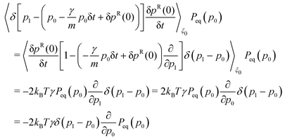 | (A9) |
where we used
eqn (A3). Linear terms in δ
pR(0) vanish as 〈δ
pR(0)〉
ξ0 = 0. Since the equilibrium distribution is Maxwellian,
i.e.,
Peq ∝ exp[−
p2/(2
mkBT)], therefore we have,
| |  | (A10) |
The integration over
p1 can then be readily performed to get
| |  | (A11) |
q.e.d. Note the small shift in δ
t between the correlations, which cannot be seen if a continuous time is taken. However, for a discrete algorithm, the shift can be appreciated in the initial stages of the decay shown in
Fig. 4.
Although the example considered here is specific, its generality can be seen if we recall that, by virtue of the FDT, the random contribution is related to the dissipative contribution. Thus, in our example it holds that
| |  | (A12) |
but it is equally true for any type of Langevin equation where the dissipative interaction is given by Onsager's linear theory. In fact, within the previous expressions conceived
as distributions, we can formally equate
| |  | (A13) |
where the stochastic term within its average can be replaced by the gradient of an appropriate
thermodynamic potential, which eventually gives rise to the diffusive term in the associated Fokker–Plank equation. Thus taking the Fokker–Plank equation for the standard DPD algorithm to easily identify the equivalent potential and for the stress tensor correlation function, we can establish
| |  | (A14) |
which, used in the expression 〈
ΠC,Dzx(
t)
ΠRzx〉 produces
eqn (44); here
Γ denotes the phase space state point of the system.
Acknowledgements
The authors would like to thank Prof. F. Schmid and Dr G. Jung for making their data available. Research performed by JBA and ADM was sponsored by the Army Research Office under Cooperative Agreement Number W911NF-20-2-0227 and Grant PID2021-122187NB-C33 funded by MCIN/AEI/10.13039/501100011033 and ERDF A Way of Making Europe. Research performed by ML was sponsored by the Army Research Office under Cooperative Agreement Number W911NF-20-2-0203. JKB and JPL acknowledge support in part for a grant of computer time from the DoD High Performance Computing Modernization Program at the Army, Navy, and Air Force Supercomputing Resource Centers.
Notes and references
- A. Einstein, Ann. Phys., 1905, 322, 549–560 CrossRef.
- E. Helfand, Phys. Rev., 1960, 119, 1 CrossRef.
-
M. P. Allen and D. J. Tildesley, Computer Simulation of Liquids, Clarendon Press, Cambridge, UK, 2017 Search PubMed.
- F. Müller-Plathe, J. Chem. Phys., 1997, 106, 6082–6085 CrossRef.
- C. Nieto-Draghi and J. B. Avalos, Mol. Phys., 2003, 101, 2303–2307 CrossRef CAS.
- A. P. Thompson, H. M. Aktulga, R. Berger, D. S. Bolintineanu, W. M. Brown, P. S. Crozier, P. J. in 't Veld, A. Kohlmeyer, S. G. Moore, T. D. Nguyen, R. Shan, M. J. Stevens, J. Tranchida, C. Trott and S. J. Plimpton, Comput. Phys. Commun., 2022, 271, 108171 CrossRef CAS.
- P. J. Hoogerbrugge and J. M. V. A. Koelman, Europhys. Lett., 1992, 19, 155–160 CrossRef.
- P. Español and P. Warren, Europhys. Lett., 1995, 30, 191–196 CrossRef.
- R. D. Groot and P. B. Warren, J. Chem. Phys., 1997, 107, 4423–4435 CrossRef CAS.
- I. Pagonabarraga and D. Frenkel, J. Chem. Phys., 2001, 115, 5015 CrossRef CAS.
- P. B. Warren, Phys. Rev. E: Stat., Nonlinear, Soft Matter Phys., 2003, 68, 066702 CrossRef CAS PubMed.
- S. Merabia, J. B. Avalos and I. Pagonabarraga, J. Non-Newton. Fluid Mech., 2008, 154, 13–21 CrossRef CAS.
- J. B. Avalos and A. D. Mackie, Europhys. Lett., 1997, 40, 141–146 CrossRef CAS.
- P. Español, Europhys. Lett., 1997, 40, 631–636 CrossRef.
- S. Y. Trofimov, E. L. Nies and M. A. Michels, J. Chem. Phys., 2005, 123, 144102 CrossRef CAS PubMed.
- M. Lísal, J. K. Brennan and J. B. Avalos, J. Chem. Phys., 2011, 135, 204105 CrossRef.
- A. F. Jakobsen, J. Chem. Phys., 2005, 122, 124901 CrossRef.
- S. Chen and X. Yong, J. Chem. Phys., 2018, 149, 94904 CrossRef.
- Z. Li, Y.-H. Tang, H. Lei, B. Caswell and G. E. Karniadakis, J. Comput. Phys., 2014, 265, 113–127 CrossRef CAS.
- J. B. Avalos, M. Lísal, J. P. Larentzos, A. D. Mackie and J. K. Brennan, Phys. Chem. Chem. Phys., 2019, 21, 24891–24911 RSC.
- J. B. Avalos, M. Lísal, J. P. Larentzos, A. D. Mackie and J. K. Brennan, Phys. Rev. E, 2021, 103, 062128 CrossRef.
- M. Lísal, J. P. Larentzos, J. B. Avalos, A. D. Mackie and J. K. Brennan, J. Chem. Theory Comput., 2022, 18, 2503–2512 CrossRef.
- E. Moeendarbary, T. Y. Ng and M. Zangeneh, Int. J. Appl. Mech., 2009, 01, 737–763 CrossRef.
- P. Español and P. B. Warren, J. Chem. Phys., 2017, 146, 150901 CrossRef.
- K. P. Santo and A. V. Neimark, Adv. Colloid Interface Sci., 2021, 298, 102545 CrossRef CAS.
- P. Español, Phys. Rev. E: Stat. Phys., Plasmas, Fluids, Relat. Interdiscip. Top., 1995, 52, 1734–1742 CrossRef.
- M. H. Ernst and R. Brito, Europhys. Lett., 2006, 73, 183–189 CrossRef CAS.
- G. Jung and F. Schmid, J. Chem. Phys., 2016, 144, 204104 CrossRef PubMed.
- M. Panoukidou, C. R. Wand and P. Carbone, Soft Matter, 2021, 17, 8343–8353 RSC.
- D. C. Malaspina, M. Lísal, J. P. Larentzos, J. K. Brennan, A. D. Mackie and J. B. Avalos, Phys. Chem. Chem. Phys., 2023, 25, 12025–12040 RSC.
- N. Lauriello, J. Kondracki, A. Buffo, G. Boccardo, M. Bouaifi, M. Lsal and D. Marchisio, Phys. Fluids, 2021, 33, 073106 CrossRef CAS.
- N. Lauriello, G. Boccardo, D. Marchisio, M. Lsal and A. Buffo, Comput. Phys. Commun., 2023, 291, 108843 CrossRef CAS.
- L. Onsager and S. Machlup, Phys. Rev., 1953, 91, 1505–1512 CrossRef CAS.
-
S. R. de Groot and P. Mazur, Non-equilibrium Thermodynamics, Dover Publications, INC, 1984 Search PubMed.
-
J. P. Hansen and I. R. McDonald, Theory of Simple Liquids, Elsevier, 2006 Search PubMed.
-
R. Zwanzig, Molecular fluids, Proceedings from the Cours d'Eté de l'Ecole de Physique Théorique, Les Houches, London, 1973, pp. 5–36 Search PubMed.
- J. B. Avalos and A. D. Mackie, J. Chem. Phys., 1999, 111, 5267–5276 CrossRef CAS.
- A. D. Mackie, J. B. Avalos and V. Navas, Phys. Chem. Chem. Phys., 1999, 1, 2039–2049 RSC.
- J. B. Avalos, M. Lísal, J. P. Larentzos, A. D. Mackie and J. K. Brennan, J. Chem. Theory Comput., 2022, 18, 7639–7652 CrossRef CAS PubMed.
- M. Lísal, J. B. Avalos, J. P. Larentzos, A. D. Mackie and J. K. Brennan, J. Chem. Theory Comput., 2022, 18, 7653–7670 CrossRef PubMed.
-
D. Frenkel and B. Smit, Understanding Molecular Simulation: From Algorithms to Applications, Academic Press, 1st edn, 2002 Search PubMed.
-
N. G. van Kampen, Stochastic Processes in Physics and Chemistry, North Holland, 1992 Search PubMed.
Footnote |
| † More general cases exist, where fluxes and thermodynamic forces are coupled; see ref. 34 and35 for details. |
|
| This journal is © the Owner Societies 2024 |
Click here to see how this site uses Cookies. View our privacy policy here. 
 Open Access Article
 This Open Access Article is licensed under a Creative Commons Attribution-Non Commercial 3.0 Unported Licence
 bc,
J. P.
Larentzos
d,
J. K.
Brennan
d,
A. D.
Mackie
bc,
J. P.
Larentzos
d,
J. K.
Brennan
d,
A. D.
Mackie


 . Eqn (4) is not a closed equation as long as JA remains undefined. Phenomenological equations, analogous to eqn (1) for the energy transport, are required to provide a closure that will produce a well posed equation for the evolution of A. In the framework of Onsager's theory of linear irreversible thermodynamics,33,34 the closure is given in the form of a linear relation between the flux and the thermodynamic forces. For the simple case analysed here as a proof of concept, we consider that the thermodynamic force can be written as a gradient of A, in analogy with Fourier's law for the heat transport or Newton's law for the shear viscosity.† Hence, the flux density becomes,

 .
.

 in terms of the dynamics of the fields, i.e.,
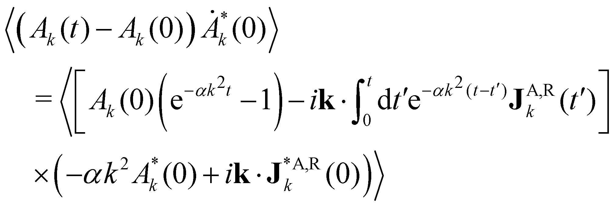
 . As a consequence, the product of the initial conditions is
  and can be neglected. Therefore, the leading contribution in the hydrodynamic limit becomes,
 . In deriving the last equality, we used eqn (10). In addition, we considered that the integration of the correlation
  over time with t′ ≥ 0 introduces a factor of 1/2 due to causality applied on the even Dirac's δ-function.36 Using eqn (6) for Ȧk(0) and the formal solution, eqn (11), with k2t → 0, we get


 (see eqn (18) and (20)). Hence, unlike in conservative systems, DPD trajectories strongly depend on the size of δt.

 , from eqn (15) we finally obtain,
 . The DPD systems contained N = 20


 , where ΠR,rzx(t)Πrzx is the value of the product along one particular system trajectory r. Then according to elementary statistical inference theory
 samples, and then another DPD simulation with a smaller timestep δt′ < δt. To have the same precision as in the former, the latter requires a larger number of samples, i.e.
 . This fact impairs a practical use of the standard formula eqn (15) to obtain the viscosity, as the size of the sampling required may become computationally unaffordable. Therefore, although the viscosity coefficient for the DPD model exists and is well defined as an overall dynamic coefficient, independent of the time-step, its determination from the statistical methods underlying the Green–Kubo expression can be strongly impaired by data dispersion, which crucially depends upon the size of the time-step. Such inherent difficulty can be strongly reduced by singling out the contribution eqn (39) from the rest of the correlation, which does not suffer from such statistical impairment.

 and
and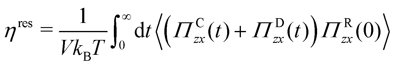


 and therefore, every element of the sum tends to zero as δt → 0. In contrast, in the standard GK formula the elements intervening in the correlation function are
  . Therefore, their dispersion increased as δt decreased, causing the evaluation of the correlation to become more difficult (see Fig. 3). The use of the EH formula requires no decomposition to reduce the statistical noise,30 and there is no need for a specific combination of stress–tensor contributions to be introduced, which differs from the approach in ref. 27.