
 Open Access Article
 This Open Access Article is licensed under a Creative Commons Attribution-Non Commercial 3.0 Unported Licence
Assessing reservoir performance for geologic carbon sequestration in offshore saline reservoirs†
Lars
Koehn
 *a,
Brian W.
Romans
a and
Ryan M.
Pollyea
ab
*a,
Brian W.
Romans
a and
Ryan M.
Pollyea
ab
aDepartment of Geosciences, Virginia Polytechnic Institute and State University, Blacksburg, VA 24061, USA. E-mail: larsk@vt.edu
bVirginia Center for Coal & Energy Research, Virginia Polytechnic Institute and State University, Blacksburg, VA 24061, USA
First published on 2nd November 2023
Abstract
Carbon capture and storage (CCS) is a technological strategy to reduce CO2 emissions from hydrocarbon-based energy production and non-energy industrial emitters, like fertilizer and cement production. To expand the geographic opportunities for CCS, offshore geologic settings are increasingly considered for saline CO2 storage, particularly where legacy oil and gas infrastructure may be repurposed for CO2 transport and injection. In this context, the Gulf of Mexico (GoM), United States (U.S.), may offer tremendous opportunity for CCS because the surrounding states are among the largest CO2 producers in the U.S. and there has been extensive oil and gas development over the last half century. Nevertheless, there remains significant uncertainty in how GoM reservoir/seal systems will respond to industrial-scale CO2 injections, particularly in the context of meso-scale (1–10s of meters) permeability variations that are difficult to identify prior to injection. Such permeability variations can have significant impacts on CO2 migration and fluid pressure propagation, both of which govern the overall effectiveness of the CCS project. This research uses ensemble simulation methods to quantify the influence of spatially variable and a priori unknown permeability fields on CO2 plume development and fluid pressure propagation when CO2 is injected at 1 MMt per year for ten years. Results show a number of characteristic patterns that reveal the substantial influence of both near- and far-field permeability on reservoir performance. By focusing on basin characteristics that are common among offshore basins worldwide, results from this study suggest that offshore CCS may be a feasible carbon management strategy in regions where offshore basins are proximal to industrial CO2 sources.
Introduction
Carbon capture and storage (CCS) is the process of capturing point- or nonpoint-source CO2 and injecting it into deep geologic reservoirs to prevent the CO2 from entering the atmosphere. Potential reservoirs include porous and permeable sedimentary rocks and fractured mafic rocks.1,2 Like hydrocarbon resources, a potential CO2 reservoir must have sufficient porosity and permeability to store large amounts of CO2, as well as a trap and seal system that prevents the buoyant CO2 from leaking to the surface.3 Additionally, reservoirs should have pressure–temperature conditions above the critical point for CO2, 31.0 °C and 7.3 MPa, allowing CO2 to be transported and injected at high density.3 During geologic storage, the CO2 is initially contained by the structural and/or stratigraphic traps in the geologic system and over longer time scales (100s to 1000s of years) a portion of the CO2 will dissolve into the pore fluid and form carbonate minerals. Widespread adoption of CCS technology in heavy-emitting industries has been proposed to be an important component of decarbonization strategies worldwide.4In the United States (U.S.), the Gulf of Mexico (GoM) is one of the most promising locations for offshore carbon sequestration as it holds a large potential storage volume and is located near carbon emission sources, as well as existing energy infrastructure. The Gulf of Mexico is a large sedimentary basin with a long history of oil and gas production in the U.S.5 Many of the same conditions that make the area suitable for hydrocarbon extraction also make the area suitable for CO2 storage, including several porous sedimentary units that are overlain by extensive low permeability shale formations that may be considered sealing units. Estimates for storage potential in U.S. Gulf of Mexico Federal waters range from 490 to 6454 billion metric tonnes of CO2.6 The low-end estimate is enough storage to potentially hold 100 years of annual CO2 emissions from the entire United States.7 In addition to the large storage volume, there are numerous large-scale CO2 producers near the Gulf of Mexico, which could facilitate the creation of commercial CCS projects. Moreover, Texas, Louisiana, and Florida rank first, second, and third, respectively, in CO2 emissions by state and the proximity of numerous large CO2 emitters to the GoM would reduce the cost of transport of CO2 for storage projects, potentially increasing the economic viability of an offshore CO2 storage hub.7 This source-sink compatibility is enhanced because numerous energy companies already operate in the region. These operators have extensive subsurface knowledge of the region and operate platforms and wells that could potentially be repurposed for CO2 injection, further reducing the cost of implementation. Conversely, existing wells could also act as conduits for CO2 leakage, thus increasing the importance of risk assessment strategies that include data-rich modeling and simulation analyses.8 Source-sink CCS compatibility tools, such as SimCCS, have been developed to assist commercial operators in identifying potential locations for CCS projects and infrastructure.9 Past studies of the GoM have rated the region as highly favourable for CCS in terms of source-sink compatibility.10 Overall, the significant advantages of the Gulf of Mexico for CO2 storage make the region a likely location for future carbon storage projects in the United States.
Among the principal challenges for any CCS feasibility assessment is to model reservoir performance on the basis of incomplete knowledge, particularly in the context of reservoir hydraulic properties. This challenge arises because CCS reservoirs occur at depths exceeding 800 m, where high pressure and temperature allow for CO2 to be injected in a supercritical state. In this context, reservoir permeability is perhaps the most difficult property to constrain because it is scale dependent,11 it can vary by several orders of magnitude within a given formation,12 and plays a fundamental role in both CO2 plume development and injection pressure propagation.13,14 At field scales, in situ reservoir permeability measurements can be taken at well sites; however, these measurements do not account for far-field permeability changes away from the well. Nevertheless, spatially variable and a priori unknown permeability fields have impacted past CCS projects, including Sleipner and In Salah. At Sleipner, Statoil (now Equinor) began storing CO2 separated from produced natural gas in the North Sea beginning in 1996.15,16 The project injected CO2 into a sandstone reservoir, the Utsira Sand, which is overlain by several hundred meters of shale caprock. The storage project was successful but seismic reflection surveys conducted after injection revealed several thin shale baffles within the sand reservoir. These baffles were too thin to be resolved in the seismic reflection data prior to injection and were not incorporated into any pre-injection planning or modeling.16 While these baffles actually improved the efficacy of the project, as they impeded flow away from the well making it easier to monitor the CO2 plume, they illustrate how small-scale heterogeneous features can have significant impacts on CCS projects. In contrast, the effects of heterogeneous permeability fields at In Salah resulted in a less successful outcome. At In Salah, BP developed an onshore CCS project in central Algeria. While this project did successfully store 3.4 Mt CO2, injection was halted prematurely due to geophysical risks.17 Specifically, reservoir fluid pressures rose faster than was predicted by pre-injection modeling. This pressure front either triggered an existing fracture network or hydraulically fractured the reservoir rock causing the operators to end the project.17 In this case, an a priori unknown and heterogenous permeability field led to higher than expected pressures forcing the cancellation of the project to avoid potential leakage. These examples illustrate the outsized role that permeability play in the success or failure of commercial scale CCS projects; at Sleipner unidentified features assisted storage efforts, while at In Salah unidentified features led to prematurely ending the project. Both examples demonstrate the importance of reservoir characterization for CO2 storage.
Past stochastic modelling studies have also demonstrated the impact that heterogeneities in reservoir properties may have on CO2 storage projects. Deng et al. (2012) and Dai et al. (2014) performed stochastic simulations with variable permeabilities and porosities for the Rock Springs Uplift, Wyoming and Kevin Dome, Montana sites respectively. These studies demonstrated that permeability and porosity magnitude and distribution exert significant control over CO2 injectivity area of review, CO2 plume geometry, leakage risk, and reservoir pressure buildup.18,19 Dai et al. (2018) performed a regional-scale CO2 storage assessment of the GoM using stochastic simulations with variable permeability, porosity, and reservoir thickness.20 This study found that heterogenous sediments may deter CO2 migration, reduce leakage risk, and potentially increase the total storage capacity of the Gulf of Mexico region.20 Finally, Pollyea and Fairley (2012), Pollyea et al. (2014) and Jayne et al. (2019b) studied the effects of spatially variable permeability on CO2 storage in fractured basalt reservoirs.14,21,22 These works developed ensemble simulations using highly correlated permeability fields built from observed fracture patterns at their respective study sites and found that variance in CO2 saturation in a CO2 storage reservoir is greatest in two concentric rings, one near the injection well and one at the edge of the simulated CO2 plume.14,21,22 Offshore commercial CO2 storage projects such as Sleipner in the North Sea and Snøhvit in the Barents Sea demonstrate the feasibility of CO2 storage in offshore saline reservoirs.15,16,23 Previous simulation studies of offshore systems, including assessments of the GoM,10,20,24 as well as other offshore basins25–27 have further supported the feasibility of CCS in offshore saline environments. This study will build from these past works by studying how spatially variable permeability affects CO2 storage in an offshore GoM sandstone system when the permeability distribution is spatially uncorrelated (random) and a priori unknown but constrained by field data from analogous GoM sandstone formations.
This study aims to quantify the effects that spatially variable reservoir features have on CCS reservoir performance by simulating CO2 injection into a heterogenous, offshore reservoir. This study is based on the Gulf of Mexico because it is widely recognized as a promising location for offshore CO2 storage; however, this study focuses on structural and stratigraphic features that are common among offshore basins worldwide. Structural, lithologic, and geologic features are simulated on the basis of variable petrophysical properties, e.g., permeability, porosity, etc. Unidentified reservoir features are simulated by generating fifty equally probable and spatially random permeability fields that are constrained on a field-scale permeability distribution from well tests originating in Miocene sandstone formations in the central Gulf of Mexico. Reservoir performance is then evaluated by combining Monte Carlo simulation with ensemble analysis (e-type) methods. Results illustrate the effects of spatially variable and a priori unknown permeability distributions within the CCS reservoir, while identifying several characteristic reservoir performance features that may occur when CO2 is injected into any porous geologic media. Specifically, this study adds further evidence that in CO2 storage reservoirs with spatially random permeability fields, the development of a relative permeability feedback plays a fundamental role in CO2 migration and that temperature monitoring is a robust and cost-effective strategy for predicting CO2 breakthrough. Furthermore, this study shows that the pattern of concentric rings of high variance in CO2 saturation previously identified in studies of highly correlated permeability fields in fractured basalts is also present in stochastic simulations with uncorrelated permeability fields in saline reservoirs.
Methods
Model construction
The geologic model for this study is based on the Main Pass and Breton Sound leasing blocks of U.S. federal waters in the Gulf of Mexico (Fig. 1). This site was selected because it reflects geological features that are characteristic of the continental shelf segment of the central Gulf of Mexico and shallow offshore basins worldwide, e.g., salt structures, faults, and alternating sandstone-shale facies, as well as publicly available geophysical data to constrain reservoir and seal geometry. The study area is also located near large CO2 producers in the Louisiana Chemical Corridor and has been developed for oil and gas extraction.28 As a result, there is substantial oil and gas infrastructure that could potentially be repurposed for CO2 transportation and injection. Additionally, a 3D seismic reflection survey was commissioned by the U.S. government to determine the value of the offshore leases and this survey is publicly available through the United States Geological Survey and The National Archive of Marine Seismic Surveys.29 We mention here that our study is not meant to generate a detailed stratigraphic and structural interpretation of this specific study site. Instead, we are using the first-order geologic features identified from the seismic-reflection survey, including interbedded Miocene layers and normal faults, as well as ensemble simulations with stochastic permeability distributions to construct a model that is broadly representative of shallow offshore basin environments, particularly the Gulf of Mexico continental shelf.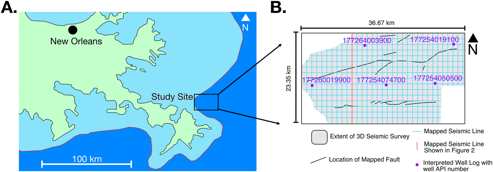 | ||
| Fig. 1 Location of selected study site in the Gulf of Mexico (A). The red boundary in Panel A indicates the border between Louisiana state waters, shown in light blue, and U.S. federal waters, shown in dark blue. Panel B shows the extent of the 3D seismic survey with the seismic lines and well logs that were used to interpret the site's geology and build our model. The red line indicates the location of the seismic line in Fig. 2 within the study site. Interpretations of the well logs shown in Panel B are included in the ESI† (Fig. S1–S5). | ||
The ∼850 km2 3D seismic-reflection survey includes 844 east-west and 1985 north-south lines with a maximum depth of 8 seconds two-way-travel-time (s TWT). Initial analysis of the 3D seismic-reflection survey found the study area to be generally representative of the central Gulf of Mexico continental shelf, e.g., bedding attitude characterized by undulating structure-contour relief associated with salt diapirism, and normal faults. An interval of high-amplitude continuous reflectors was identified within the seismic survey between 1.2 and 2.5 TWT s depth, where temperature and pressure conditions are likely suitable for carbon storage. High-amplitude reflectors are the result of a strong contrast in the impedance properties (density and velocity) of the rock, indicating a contact between units of differing physical properties, such as the contact between a sandstone and a shale. Additionally, using an average seismic velocity of 1700 m s−1 (5577 ft per s), this interval is at an approximate depth of 1020–2125 m below the mudline, which is a sufficient depth to store CO2 in a supercritical state. The lithologic variability of this interval was characterized using spontaneous potential and gamma ray well logs from legacy oil and gas wells (Fig. S1–S5, ESI†). Within this interval of interest, six seismic horizons, delineating a ∼130 m-thick interbedded sandstone-shale package, were mapped continuously across the study area. These horizons form the basis for the sediment layers within the geologic model (Fig. 2). The 3D seismic survey also revealed the presence of 12 normal faults, which have been included into the geologic model (e.g., see Fig. 1 and 2).
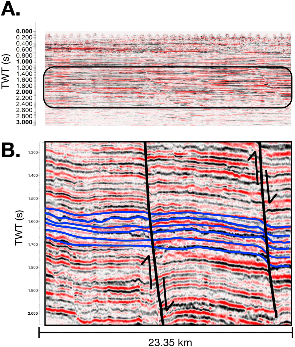 | ||
| Fig. 2 An example crossline from the selected 3D seismic survey. The depth interval of interest is shown in Panel A. Panel B contains mapped horizons within that interval in blue and mapped faults are shown in black. The spatial coordinates of these mapped features were exported from the seismic software and used to define geologic features in our model. Refer to Fig. 1 for the location of this seismic line. | ||
Well data from the Bureau of Ocean Energy Management (BOEM) Gulf of Mexico Sands Atlas indicates that the depth interval described above is within the Upper Miocene.30 Hentz and Zeng (2003) studied the sequence stratigraphy of the Gulf of Mexico continental shelf at a site to the west that is in a generally similar position as our study area with respect to the modern shoreline and, thus, is a reasonable depositional analog. They characterized these sediments as interbedded packages of sandstone and shale.31 Therefore, the mapped horizons were interpreted to represent the contacts between interbedded layers of sandstone-dominated and shale-dominated units, which form the basis for a reservoir (sandstone-dominated) and seal (shale-dominated) system in the context of geologic CO2 storage.
The mapped horizons and faults are used to construct a discretized geologic model in the reservoir simulator, PetraSim.32 The simulation grid has an approximate area of 856![[thin space (1/6-em)]](https://www.rsc.org/images/entities/char_2009.gif) 101 km2 and a maximum depth of 2125 m below mudline. The mapped horizons define interbedded layers of a sandstone-shale package that includes three shale and two sand layers. The model also includes a coarsely discretized overburden layer that exists from the top of the upper shale layer to the mudline. This overburden layer is included in the model domain to allow for thermal and hydraulic communication between the target reservoir and hydrostatic upper boundary condition, thus mitigating the potential for non-physical feedbacks propagating from the upper boundary condition.
101 km2 and a maximum depth of 2125 m below mudline. The mapped horizons define interbedded layers of a sandstone-shale package that includes three shale and two sand layers. The model also includes a coarsely discretized overburden layer that exists from the top of the upper shale layer to the mudline. This overburden layer is included in the model domain to allow for thermal and hydraulic communication between the target reservoir and hydrostatic upper boundary condition, thus mitigating the potential for non-physical feedbacks propagating from the upper boundary condition.
The model domain is discretized into approximately 960000 grid cells using Voronoi tessellation in the horizontal plane and regular discretization in the vertical direction (Fig. 3). The injection site is located in the approximate center of the domain, with a completion interval of 1870–1902 m depth below the mudline. Additionally, grid cells are refined to an area of 1.5 m2 adjacent to the injection site. This refinement allows for greater resolution and accuracy of thermophysical behavior in early simulation time. Grid cell area increases away from the injection site to a max grid cell area of 100000 m2 at 50 m from the injection site. The resulting geologic model comprises a coarse representation of alternating layers of sandstone- and shale-dominated units that reflect the presence of first-order, map-scale geologic structures, such as faults and folds.
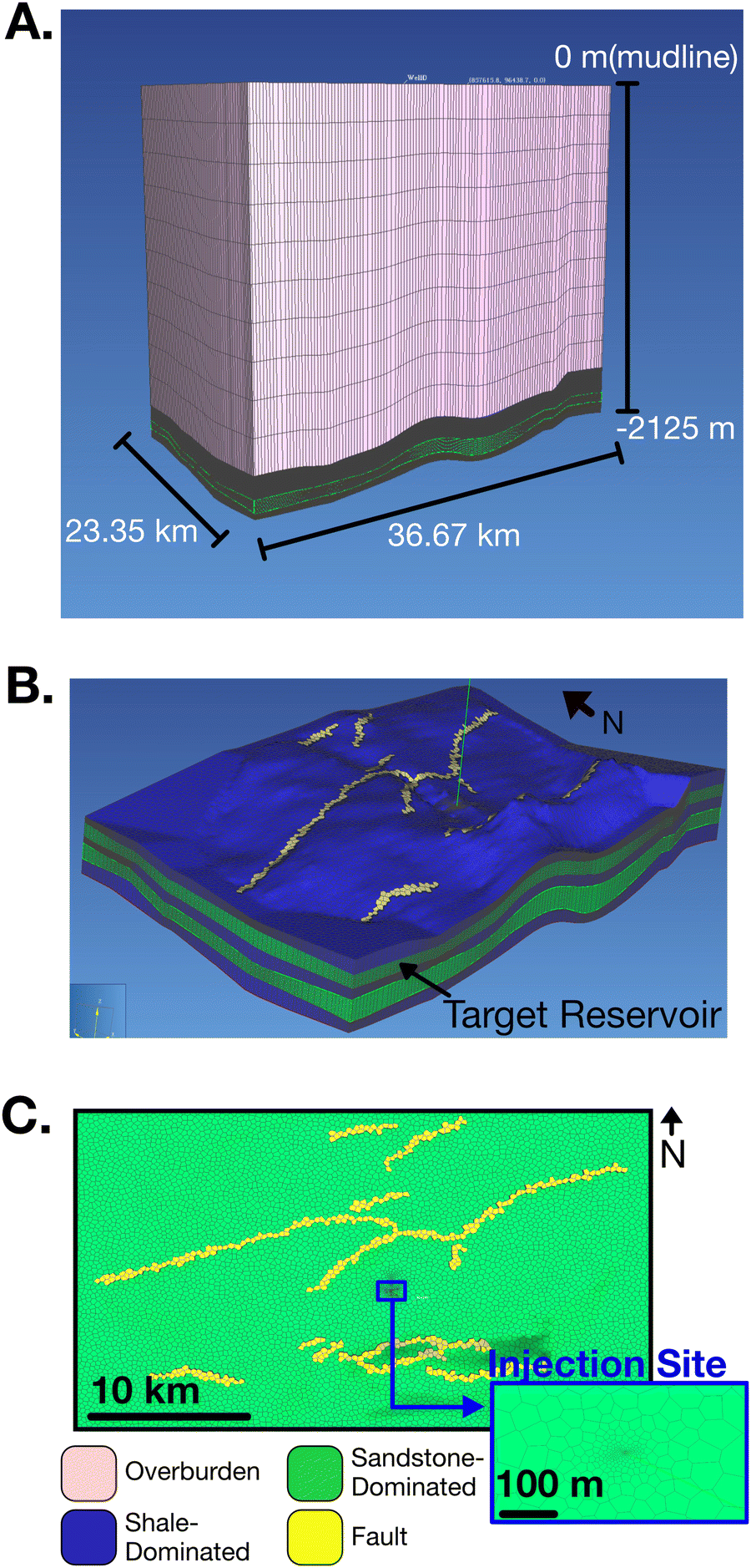 | ||
| Fig. 3 Geologic model utilized for this study. Panel A displays the full geologic model with overburden layers to maintain hydraulic communication with the upper boundary (Note 20× vertical exaggeration). The reservoir-seal system is highlighted in (B) with reservoir rock (sandstone-dominated) in green and seal rock (shale-dominated) in blue. The top of the target reservoir is shown in (C) to illustrate the grid refinement near the injection well and the fault system that is discretized into the model domain. | ||
The objective of this study is to assess reservoir performance during CO2 injection in the central Gulf of Mexico when the spatial distribution of permeability is a priori unknown within the target reservoir. To meet this objective, a distribution of permeability from Miocene sandstone is compiled using field-scale permeability data from the BOEM Gulf of Mexico Sands Atlas (Fig. 4A).30 This dataset shows that Miocene sandstone within the Gulf of Mexico (n = 690) is characterized by a mean permeability of 2.51 × 10⁻¹³ m2 and standard deviation of 7.65 × 10⁻¹³ m2. The general characteristics of the seismic-reflection data (aided by our horizon mapping) indicates that the interval of interest is not characterized by systematic lateral sedimentary facies changes or significant channelization (Fig. 2), which allows us to assume that any spatial correlation within the permeability structure occurs at length scales smaller than the grid cell dimensions. On this basis, fifty (50) individual model domains were generated by assigning the permeability of each reservoir grid cell (Fig. 3B) as a random draw from the BOEM distribution. The vertical permeability of each cell is reduced by one order of magnitude to account for thinly bedded shales that are common in this setting and may impede vertical flow. The fifty unique model domains are identical in all aspects, except for the spatial permeability distribution in the CO2 storage reservoir. Fig. 4B–D illustrates the permeability distributions for three of the fifty reservoir models and Fig. 5 illustrates a plan-view slice of the permeability structure at 1880 m depth for each permeability distribution shown in Fig. 4B–D.
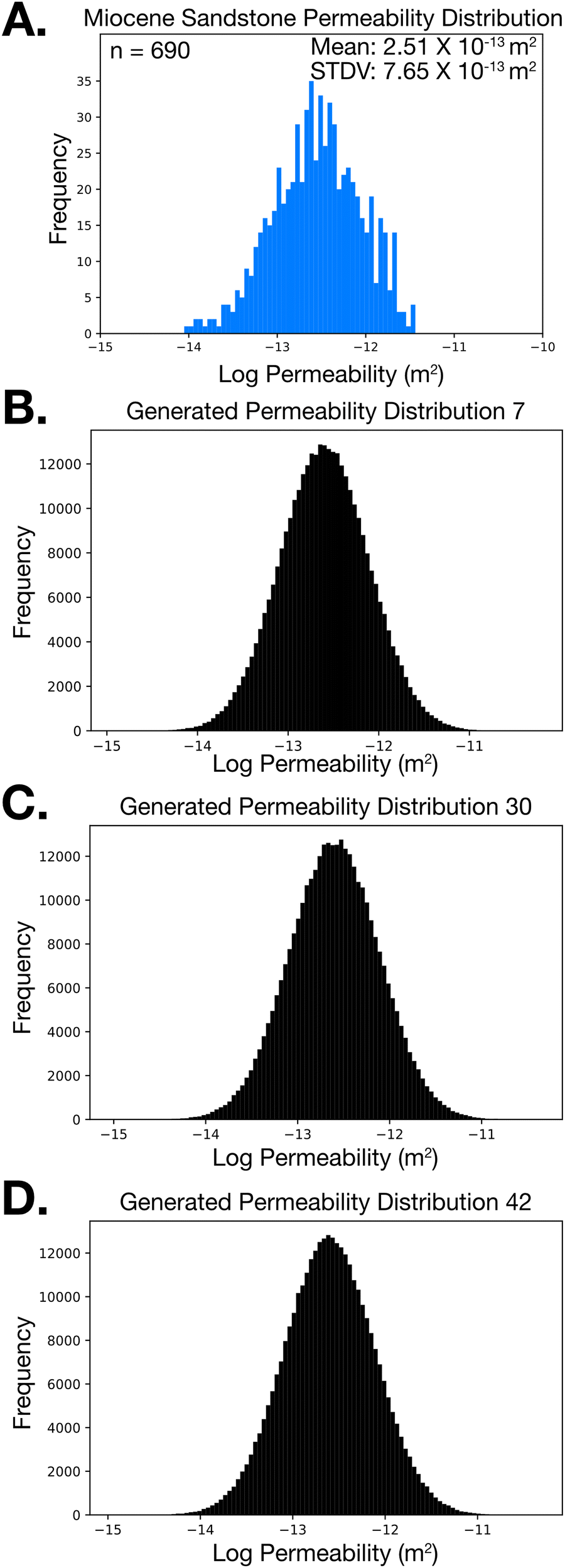 | ||
| Fig. 4 Comparison of permeability distribution from the Miocene sand reservoirs (Panel A) with examples of three synthetic permeability distributions from the simulation ensemble (Panels B–D). Note that 50 synthetic permeability distributions were generated for this study and the permeability distribution of Miocene sand reservoirs is from the BOEM Atlas. | ||
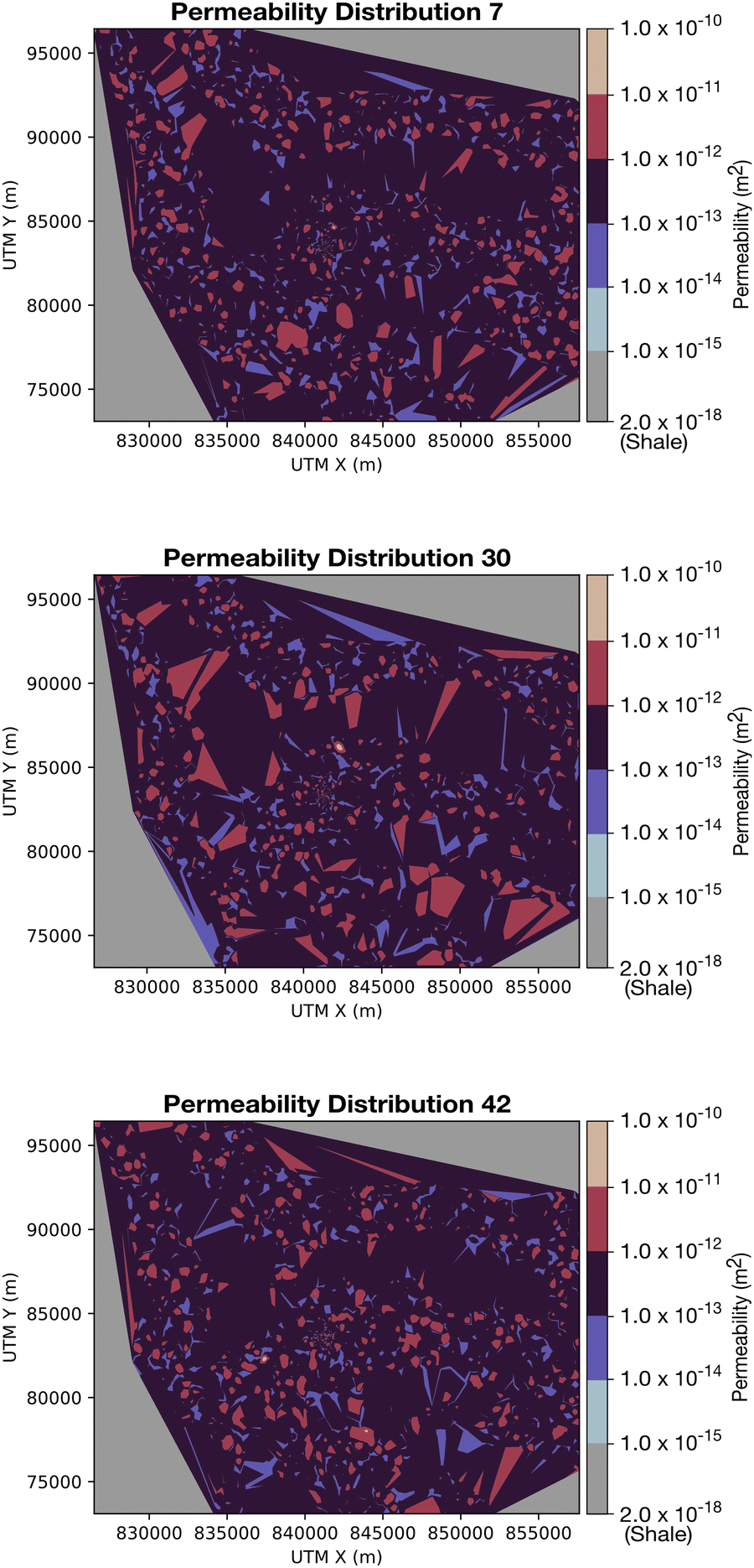 | ||
| Fig. 5 Permeability contours of three model realizations. Each image is a cross-section of the model at 1880 m depth showing the spatially variable permeability within the sandstone reservoirs. Each permeability structure is assigned randomly with no spatial correlation. | ||
The remaining petrophysical rock properties are assigned based on literature values for analogous lithologies (Table 1). Shale permeability and porosity are assigned based on values from Lu et al. (2017) and sandstone porosity is assigned using the average of Miocene reservoir porosities from the BOEM Atlas.30,33 As the overburden layer includes undifferentiated sandstone and shale, it is assigned anisotropic permeability using data from both lithologies. Specifically, overburden lateral permeability is set equal to the average permeability of Miocene sands from the BOEM Atlas as lateral flow would be dominated by sandstone lithologies. We observe strong evidence for thin interbedded shales in the target reservoir interval in the geophysical data for our study site and we expect these interbedded shales to act as baffles impeding vertical flow. In the absence of anisotropic permeability measurements, we used 1 order of magnitude reduction in vertical permeability to account for this flow impediment. Fault permeability reflects the observed phenomenon that faults act as cross-strike barriers to flow due to the presence of low permeability fault gouge.34 Petrophysical properties for the different lithologies are summarized in Table 1.
| Lithology | k xy (m2) | k z (m2) | Porosity | ρ (kg m−3) | κ (W m−1 °C) | c (J kg−1 °C) |
|---|---|---|---|---|---|---|
| k xy = horizontal permeability; kz = vertical permeability; porosity is unitless; ρ = density; κ = thermal conductivity; c = specific heat. | ||||||
| Sandstone-dominated | Variable | 0.1 × kxy | 0.31 | 2350 | 2.37 | 710 |
| Shale-dominated | 2.0 × 10⁻¹⁸ | 2.0 × 10⁻¹⁸ | 0.20 | 2450 | 1.50 | 770 |
| Overburden | 2.5 × 10⁻¹³ | 2.0 × 10⁻¹⁸ | 0.22 | 2400 | 2.37 | 710 |
| Fault | 1.0 × 10⁻¹⁸ | 1.0 × 10⁻¹⁸ | 0.20 | 2450 | 1.50 | 770 |
Van Genuchten relative permeability and capillary pressure models are used to account for the multi-phase effects of free phase CO2 and brine occupying the same pore space.35 These formulations provide a family of characteristic functions in which relative permeability and capillary pressure vary as a function of wetting-phase saturation. These functions are fit to laboratory measurements of sediment parameters like endpoint saturation values. In the absence of multi-phase rock property data for Gulf of Mexico Miocene sediments, this study uses standard relative permeability and capillary pressure curves for sandstone.36 Past studies have shown that relative permeability and capillary pressure exert significant influences over CO2 flow behavior.13,37–39 Relative permeability and capillary pressure measurements are available for several other geologic units;38,40 however these experiments were all performed on the core-scale. There remains significant uncertainty in how permeability and capillary pressure properties vary on the reservoir-scale. Further work is needed to understand how relative permeability and capillary pressure properties may vary across 100s of km3 of reservoir volume. In this study we use generic constitutive relations for relative permeability and capillary pressure but note that there are uncertainties in whether these functions apply on the reservoir-scale and whether they remain constant across the reservoir.
Prior to each simulation, initial pressure and temperature conditions are specified to be reflective of the Gulf of Mexico. The standard pressure gradient for the region is assigned as 1.05 × 10⁻² MPa m−1 (0.47 psi per ft),41 while the corresponding thermal gradient of 0.02 °C m−1 is applied on the basis of mean recorded temperature gradients from the BOEM Atlas.30 Constant pressure and temperature boundaries are imposed across the top and lateral extent of the model domain to maintain (i) constant fluid pressure at the mudline and (ii) the far-field pressure and temperature gradients. The basal boundary is adiabatic to fluid pressure and a heat flux of 50 mW m−2 is applied to account for the influx of geothermal heat.42 An initial brine concentration of 35000 ppm is assumed throughout the study area.
Injection scenario
This study considers a scenario in which supercritical CO2 is injected at 1 MMT per year for 10 years within a single injection well that is open between 1870 and 1902 m depth. This injection interval is entirely within the uppermost sandstone unit in the model domain (Fig. 3). The injection scenario is repeated for each of the fifty permeability realizations to produce an ensemble of fifty unique simulation results. Each ensemble member (simulation) comprises a permeability distribution with identical mean and standard deviation of permeability values within the target CO2 storage reservoir (Fig. 4); however, the spatial configuration of this permeability distribution is unique (Fig. 5). As a consequence, the resulting CO2 injection simulations reflect equally probable outcomes when overall spatial permeability distribution is well-constrained, but spatially uncertain. Each CO2 injection simulation is computed with the TOUGH3 numerical simulation code compiled with the equation-of-state module ECO2N v2.0 for nonisothermal mixtures of water, CO2 and NaCl.36,43 The TOUGH3/ECO2N simulator solves the mass and energy conservation equations by means of integral finite volume discretization in space and first-order finite difference in time. Phase partitioning between water, CO2, and NaCl is based on local thermodynamic equilibrium.43,44 In the context of CO2 trapping mechanisms, the modeling framework implemented for this study assesses geologic CO2 storage in the context of (i) structural/stratigraphic trapping, whereby buoyant, supercritical CO2 becomes physically trapped from above by a sealing unit that prevents vertical flow through a combination of low permeability and high capillary entry pressure, e.g., shale or anhydrite; (ii) solubility trapping, whereby a fraction of the injected CO2 dissolves into the aqueous phase, thus preventing the CO2 from escaping the disposal reservoir; and (iii) capillary (or residual gas) trapping, which is a pore-scale process that occurs during imbibition as capillary forces decrease upward mobility of small, disconnected CO2 bubbles. The authors note that this study does not consider CO2 mineral trapping, which, in sandstone, is likely to occur over timescales exceeding 103–104 years because the dissolution rate of quartz is known to be substantial limitation to this CO2 trapping process.To assess CO2 trapping characteristics and reservoir performance in the context of spatial permeability uncertainty, the complete simulation ensemble (N = 50) is analyzed on the basis of ensemble-type (e-type) methods, which compute a mean and variance within each grid cell for each dependent variable across all simulations.45 The advantage of this e-type approach over deterministic simulation methods is that uncertainty estimates are generated for all simulation output in each grid cell. For example, the ensemble mean CO2 saturation for each grid cell is accompanied by a corresponding variance, so that spatial uncertainty can be used to understand how permeability variations affect the processes governing CO2, pressure, and temperature variations. A schematic illustration of ensemble simulation with e-type analysis is shown in Fig. 6. Given the computational demands for simulating nonisothermal, multi-phase CO2-brine flow (8 to 12 hours per simulation on 256 processors), this study implements N = 50 simulations to strike a balance between robustness for e-type calculations and computational efficiency. We note that fifty realizations have been used in past CCS related ensemble studies.46,47
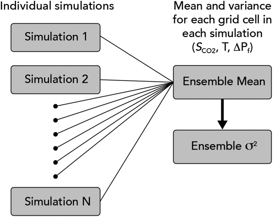 | ||
| Fig. 6 Schematic illustration of ensemble simulation analysis. | ||
Results and discussion
CO2 flow uncertainty
Results from the ensemble mean (N = 50) of CO2 saturation show that the overall plume geometry follows an expected pattern that resembles an inverted cone around the injection well. This result is expected because it is well established that CO2 migration is governed by buoyancy-driven flow in the far-field due to the density difference between lower density supercritical-phase CO2 and higher density formation brine (Fig. 7, left column).39 As a result, CO2 tends to rise within the injection reservoir and then spread laterally against the bottom of the overlying caprock. We note that that the average CO2 plume is slightly elongated in the northwest direction because the geologic units in the model are dipping slightly in south-southeast direction and because pressure buildup against bounding faults to the north and south may be driving increased lateral flow. The nature of this pressure buildup is further discussed in the section, Pressure build-up along faults.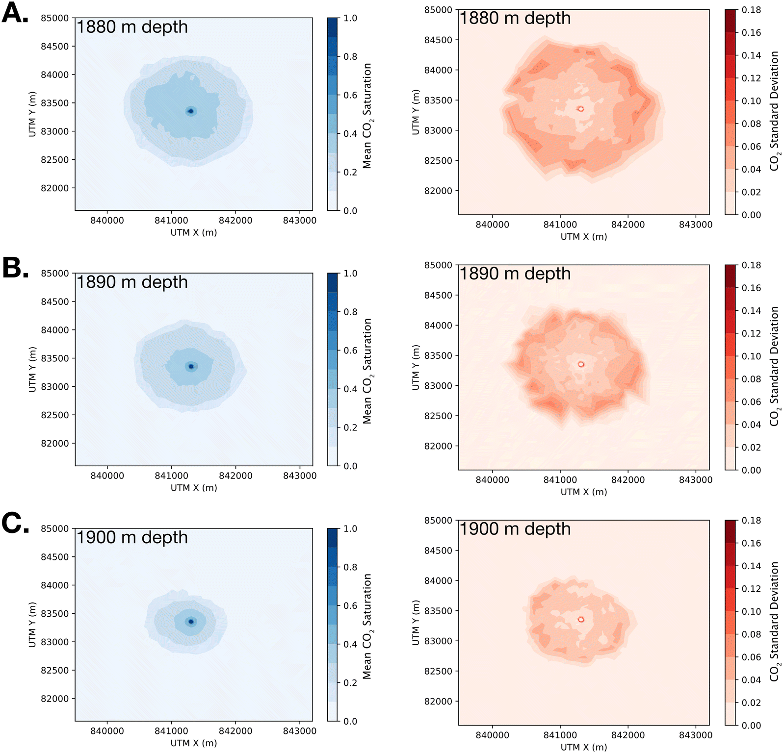 | ||
| Fig. 7 Ensemble simulation results (N = 50) for CO2 saturation at (A) 1880 m depth, (B) 1890 m depth, and (C) 1900 m depth after 10 years of CO2 injection. Mean CO2 saturation is shown on the left column with the corresponding standard deviation on the right. Note that the size of the CO2 plume increases at shallower depths because CO2 is buoyant (less dense) in brine and moves to the top of the reservoir until reaching the low permeability cap rock. | ||
Interestingly, results for ensemble standard deviation (N = 50) of CO2 saturation indicate that there are two regions in which spatial permeability uncertainty is superimposed on to CO2 flow paths; one region is in close proximity to the injection well, while the other region occurs in the far field at the leading edge of the CO2 plume (Fig. 7, right column). Specifically, the standard deviation of CO2 saturation near the injection well exhibits ±0.18 m3 m−3 CO2 saturation. This ring of high uncertainty is created by differences in near-field permeability adjacent to the injection well (Fig. 8), which cause a reinforcing feedback cycle between CO2 saturation and relative permeability.21 This reinforcing feedback develops because CO2 initially flows laterally away from injection well in the direction of highest permeability. As CO2 enters the high permeability region, the CO2 saturation increases, thus increasing the non-wetting phase relative permeability, which is CO2 in this case. This increase in non-wetting phase relative permeability further increases CO2 mobility, thus permitting additional CO2 to enter. This self-reinforcing relative permeability feedback drives CO2 flow and accumulation along preferential flow paths away from the injection well.
 | ||
| Fig. 8 Simulation results of CO2 flow rate from one injection cell into adjacent grid cells for ensemble simulations 19, 36, and 50 in early time. Panel A illustrates the spatial configuration of grid cells adjacent to the injection cell. Color codes are repeated in cells B–D, which illustrate the CO2 flow rate (kg m−2 s−1). Note that high permeability grid cells receive higher CO2 flow rates. | ||
The relative permeability reinforcing feedback process is illustrated in Fig. 8, which displays how flow paths from an injection site are impacted by near-field permeability. In Fig. 8B–D, the grid cells with the highest bulk permeability receive the largest CO2 flow rate within the first hour of injection; however, these early-time flow rates are highly variable. When this initial flow rate variability stabilizes, a consistent pattern emerges in which CO2 flow rates continue increasing for high permeability grid cells, e.g., see red and orange curves in Fig. 8B. This phenomenon is not observed for the lower permeability grid cells, in which CO2 flow rates either stabilizes or declines.
The near-field relative permeability feedback mechanism described above has been reported in past studies of ensemble CO2 storage simulations including, Ennis-King et al. (2011),48 Pollyea and Fairley (2012),21 Deng et al. (2012),18 and Jayne et al. (2019b).14 These past ensemble studies all used spatially correlated permeability fields. As a result, it was unclear if the relative permeability feedback is governed by strongly correlated permeability fields or near-field heterogeneity. Because the present study implements spatially uncorrelated permeability fields, these results demonstrate that this relative permeability feedback mechanism is likely to occur in any heterogeneous permeability distribution, regardless of whether or not the heterogeneity is spatially correlated or spatially random.
In addition to the zone of elevated uncertainty near the injection well, CO2 saturation is characterized by an additional ring of high standard deviation, ±0.10 m3 m−3 at the edge of the CO2 plume. This ring of uncertainty indicates that there are differences in the final shape and lateral extent of the CO2 plume across the fifty realizations. Since each model in the ensemble comprises identical CO2 injection volume and initial PT conditions, this uncertainty is driven by differences in far-field reservoir permeability. Specifically, this result demonstrates that spatially uncorrelated permeability fields result in uniformly concentric uncertainty patterns in the far field. This is in strong contrast to situations when permeability exhibits long-range (km-scale) spatial correlation. In this latter case, mean CO2 plume geometry and the corresponding standard deviation generally trend in the direction of maximum spatial correlation, e.g., Jayne et al. (2019b).14 In the context of monitoring, measuring, and verification (MMV), this implies that a priori knowledge of permeability correlation structure may be a leveraged to optimize MMV design plans when permeability fields are spatially correlated and this correlation structure is known. In contrast, results from the present study suggest that a priori reservoir performance insights cannot be inferred when the reservoir is characterized by spatially uncorrelated (randomly distributed) permeability fields. Nevertheless, the concentric patterns for both ensemble mean CO2 saturation and the corresponding ensemble standard deviation suggest that the overall footprint of a CO2 plume may be predictable even when far-field permeability is poorly constrained. This may have important implications for area of review criterion in the planning and permitting stages of an offshore CCS project.
Finally, we acknowledge that integral finite difference method and grid discretization used in these simulations introduces some inherent error related to numerical dispersion of mass in the model. As this simulation method calculates the mass and properties for each grid cell at the center of the cell, mass that should exist near the boundary of the cell is “shifted” to the center of the cell introducing a spatial error based on the grid spacing. In these models, the average grid spacing of the largest cells is approximately 300 m; therefore, the maximum dispersion is about 150 m. This introduces some error in the simulated distribution of CO2 and the CO2 plume size; however, we note that our simulated CO2 plume diameter is within the expected range for an injection of this volume. The mean radius of the CO2 plume in our Monte Carlo simulations is 1.05 km, which appears feasible based on results from the Sleipner storage project. For example, 4D seismic monitoring from Sleipner in 2006, ten years after injection began and at an injection volume of about 10 million metric tonnes, shows a CO2 plume with a radius of about 1 km.49 Therefore, while some numerical dispersion error exists in our simulation, our results appear feasible based on observations from Sleipner.
Temperature as an indicator for CO2 flow
The mean and standard deviation of model temperatures were also examined after 10 years of constant rate CO2 injection (Fig. 9). These results show a persistent decrease in temperature near the well, which is driven by Joule-Thompson cooling from CO2 expansion (Fig. 9A–C). In addition, there is a warming front that extends several km beyond the CO2 plume. These results are consistent with the Jayne et al. (2019a), which showed that the thermal regime surrounding CO2 injection in a homogeneous, isotropic reservoir is characterized by (i) Joule–Thomson cooling in the dry-out zone (near the injection well), where CO2 is expanding, and (ii) a broad heat front beyond the dry-out zone, where CO2 dissolution in water and to a lesser extent, Joule–Thomson heating of H2O, are the dominant thermal processes.50 The ensemble results for this study show that the mean temperature drop is ∼0.8 °C in the dry-out zone and the mean temperature increase reaches ∼1.2 °C (Fig. 9, left column). Interestingly, the standard deviation of temperature (Fig. 9, right column) indicates that temperature variability is greatest where there is a change in the dominant thermal process. In this context, both the cooling and warming fronts are primarily governed by the mass of CO2 expanding and dissolving, respectively, within the storage formation. To the first order, the CO2 mass available for these thermal processes is a function of (i) porosity, which provides physical space for CO2 and water, and (ii) permeability, which controls the rate at which CO2 can displace water in the available pore space. For this study, porosity is held constant for each simulation in the ensemble, so the CO2 mass within the pore space is controlled largely by permeability. In addition to permeability and porosity, the thermal signature associated with CO2 migration in the storage reservoir is governed by the Joule–Thomson coefficient, heat of dissolution, and CO2 solubility, which are all affected to some extent by fluid pressure variability. In a heterogeneous permeability field, lower permeability zones lead to higher fluid pressure as CO2 displaces water in the pore space.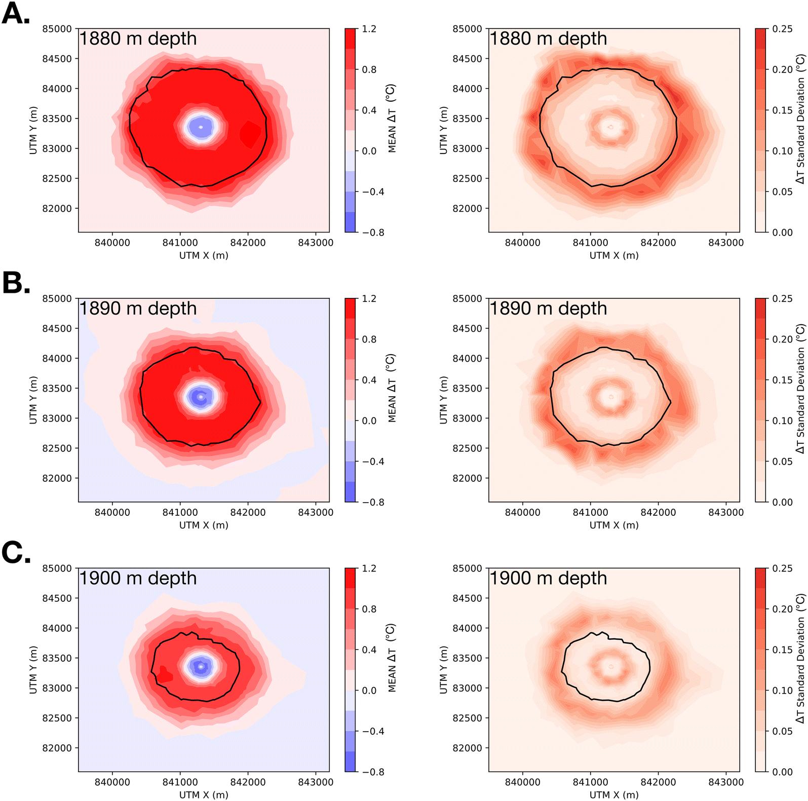 | ||
| Fig. 9 Ensemble simulation results (N = 50) of temperature changes (ΔT °C) within the injection reservoir after 10 years of CO2 injection at (A) 1800 m depth, (B) 1890 m depth, and (C) 1900 m depth. The black contour indicates the furthest extent of the free-phase CO2 plume, defined as the mean 1% CO2 saturation contour (Fig. 7). Mean ΔT is shown on the left column with the corresponding standard deviation on the right. Note that the max temperature drop (−ΔT) is −0.8 °C near the injection well (left column, blue shading) and temperature increase (+ΔT) is +1.2 °C (left column, red shading). Also note that the lateral extent of the temperature change in the reservoir is greater than the lateral extent of the CO2 plume (black contour). | ||
To understand how heterogeneous permeability fields affect fluid pressure and temperature variability within the dry-out zone, Han et al. (2010) show that the Joule–Thomson coefficient for CO2 at 50 °C varies from ∼3 °C MPa−1 at 10 MPa to ∼0.1 °C MPa−1 at 40 MPa.51 After 10 years of injection, pressure and temperature conditions within the storage reservoir range from 20 to 21 MPa and 56 to 58 °C, which corresponds with a Joule–Thomson coefficient for CO2 of ∼0.5 °C MPa−1.51 This Joule–Thomson coefficient for CO2 explains how permeability-controlled pressure variability leads to a standard deviation ±0.25 °C at the leading edge of the dry-out zone, where low permeability zones cause fluid pressure to increase, while higher permeability zones maintain lower fluid pressures. Because the Joule–Thomson coefficient for CO2 increases with decreasing fluid pressure, results from this study can be generalized to suggest that variability in the cooling front within heterogeneous reservoirs will be greater at shallow depths, where the absolute pressures are lower.
The warming front illustrated in Fig. 9 is primarily governed by the heat of dissolution, which occurs because CO2 dissolution in water is an exothermic reaction. As a result, the mass of CO2 dissolving in water plays a fundamental role in the energy released to drive this warming front. To understand how permeability-controlled fluid pressure variability affects this warming front, this study considers two mechanisms, (i) CO2 solubility in water and (ii) enthalpy released during dissolution. Duan et al. (2006) show that the solubility of CO2 in water ranges from 1.11 to 1.12 mol kgH2O−1 at pressure (20–21 MPa) and temperature (56–58 °C) conditions within the modeled reservoir.52 This suggests that CO2 solubility is relatively consistent under the fluid pressure variability imposed by the heterogeneous permeability field. In terms of energy release, Koschel et al., (2006) shows that the energy released during CO2 dissolution in water is ∼15 kJ mol−1 at the temperature conditions tested here, but this decreases to ∼8 kJ mol−1 at 100 °C.53 Because the energy release from dissolution decreases with increasing temperature and CO2 solubility decreases with increasing pressure and temperature, it is likely that the thermal effects discussed here are more pronounced at shallow depths, where CO2 sequestration will be more economically feasible.
Furthermore, the Joule–Thomson heating of water also contributes to the warming front described above. At model reservoir conditions (20–21 MPa and 56–58 °C) the Joule–Thomson Coefficient of H2O is ∼−0.207 °C MPa−1.54,55 Since the Joule–Thomson coefficient of H2O is negative, H2O expansion results in a temperature increase; the opposite effect of CO2 expansion. Based on the simulated change in reservoir pressure, ∼1.0–1.2 MPa pressure increase as discussed further in the following section, the Joule–Thomson heating of water contributes approximately 0.2 °C of warming to the system. Therefore, the dissolution of CO2 in water is the dominant heating process in the warming front, but the Joule–Thomson heating of H2O makes a significant contribution to the warming of the system.
The thermal processes discussed above occur in a transient pressure field that drives both CO2 and brine laterally away from the injection well. As pore fluid temperature increases in the far-field, the increasing pressure head drives the warm front ahead of the advancing CO2 plume. Results from this study show that the warming front appears to precede the CO2 plume in the reservoir. Comparing Fig. 7–9 shows that the average lateral extent of the warm front is greater than the extent of the CO2 plume. The black contour in Fig. 9 indicates the furthest extent of the CO2 plume from Fig. 7. To test if the warming front is a reliable precursor to the arrival of free phase CO2 within a spatially uncorrelated permeability field, we examined the time series of average temperature and CO2 concentration at four points around the ensemble mean CO2 plume (Fig. 10). For this analysis, the mean time lag (![[t with combining macron]](https://www.rsc.org/images/entities/i_char_0074_0304.gif) l) is defined as the difference between the time required for a temperature increase of 0.1 °C and CO2 saturation increase of 0.01 (1%). Put differently, l is the time difference between a change in formation temperature and arrival of the CO2 plume. Fig. 9B–E shows that l ranges from 161 days at 543 m distance from the injector to 676 days at 871 m distance. However, the robustness of these results appears to be dependent on distance from the injector. Specifically, for monitoring locations located 543 m and 643 m from the injection well, the corresponding l values are 161 days and 248 days, respectively, but these results fall within the 1σ error bars (Fig. 10C and D). In contrast, monitoring locations located 706 m and 871 m have l values of 301 days and 676 days, respectively, and these results occur well beyond the corresponding 1σ error (Fig. 10B and E). This analysis indicates that formation temperature is likely to be a leading indicator of CO2 breakthrough; however, this result appears to be more reliable at larger radial distances from the injection well. This result is consistent with Jayne et al. (2019a,b), which showed that temperature predicts CO2 breakthrough in a models comprising a single heterogeneous permeability field.14,50 In the present case, our results show that this thermal breakthrough signature is robust when considered in the context of a large (N = 50) simulation ensemble with spatially random permeability distributions. Considering Jayne et al. (2019a,b) in the combination with the robustness of the ensemble results presented here offers compelling evidence that temperature may be a cost effective strategy for predicting CO2 breakthrough in heterogeneous geologic formations.14,50
l) is defined as the difference between the time required for a temperature increase of 0.1 °C and CO2 saturation increase of 0.01 (1%). Put differently, l is the time difference between a change in formation temperature and arrival of the CO2 plume. Fig. 9B–E shows that l ranges from 161 days at 543 m distance from the injector to 676 days at 871 m distance. However, the robustness of these results appears to be dependent on distance from the injector. Specifically, for monitoring locations located 543 m and 643 m from the injection well, the corresponding l values are 161 days and 248 days, respectively, but these results fall within the 1σ error bars (Fig. 10C and D). In contrast, monitoring locations located 706 m and 871 m have l values of 301 days and 676 days, respectively, and these results occur well beyond the corresponding 1σ error (Fig. 10B and E). This analysis indicates that formation temperature is likely to be a leading indicator of CO2 breakthrough; however, this result appears to be more reliable at larger radial distances from the injection well. This result is consistent with Jayne et al. (2019a,b), which showed that temperature predicts CO2 breakthrough in a models comprising a single heterogeneous permeability field.14,50 In the present case, our results show that this thermal breakthrough signature is robust when considered in the context of a large (N = 50) simulation ensemble with spatially random permeability distributions. Considering Jayne et al. (2019a,b) in the combination with the robustness of the ensemble results presented here offers compelling evidence that temperature may be a cost effective strategy for predicting CO2 breakthrough in heterogeneous geologic formations.14,50
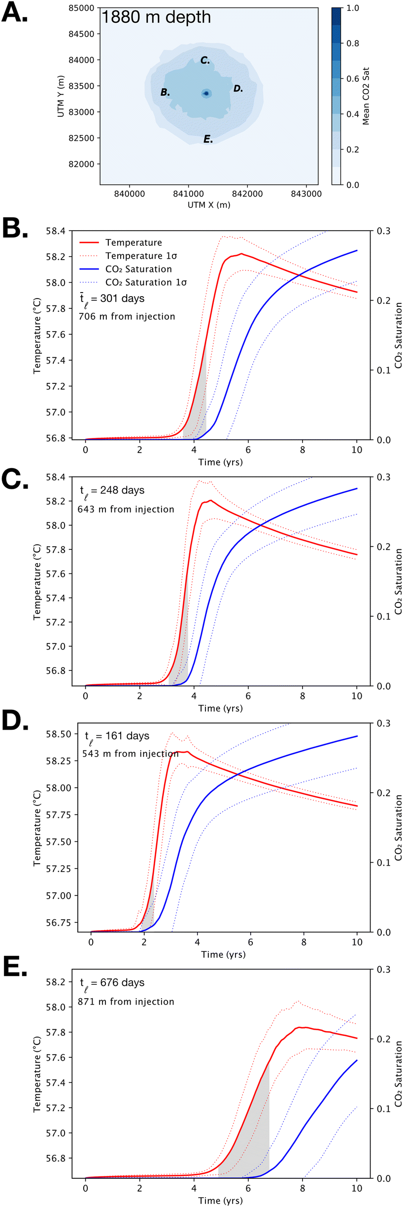 | ||
| Fig. 10 Time series of mean temperature (red curves) and mean CO2 saturation (blue curves) at four monitoring locations that are located within the CO2 storage reservoir at 1880 m depth. Monitoring locations are shown in Panel A with respect to the mean CO2 plume (blue shading) after 10 years of injection. Time series in Panels B–E correspond with locations shown in Panel A. Gray shading denotes average time lag (l) between arrival of thermal front (defined as 0.1 °C temperature increase) and arrival of the CO2 plume (defined as a 0.01 increase in CO2 saturation). | ||
Pressure build-up along faults
Changes in fluid pressure (ΔPf) were also examined in the model results (Fig. 11). For the study area evaluated here, the east-northeast trending low-permeability faults compartmentalize the advancing pressure transients to the north and south, while long range pressure transients advance to the east and west (Fig. 11A). Injection-induced fluid pressure change is of particular concern for geologic CO2 sequestration because (i) induced pressure transients are known to cause earthquakes at large radial distances from oilfield wastewater injection wells,56–58 and (ii) CO2 injections are likely to occur within geologic formations that have similar pressure and temperature regimes as oilfield wastewater disposal reservoirs.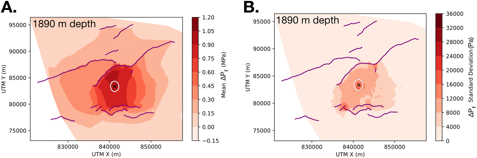 | ||
| Fig. 11 Ensemble simulation results (N = 50) of pore pressure change (ΔPf) within injection reservoir at 1590 m depth after 10 years of CO2 injection. Panel A presents mean ΔPf with the corresponding standard deviation of ΔPf shown in panel B. The CO2 injection site is marked with an × and the farthest extent of the CO2 plume is shown in white. Faults traces are shown as purple lines and modeled as low permeability barriers to fluid flow. | ||
For the model scenario developed here, ensemble simulation results show mean ΔPf of ∼1 and 1.2 MPa (±0.004–0.02 MPa) reach the faults to the north and south of the injection site after 10 years of injection, respectively (Fig. 11). In natural settings, static stress changes as low as 10 kPa have been implicated in remote earthquake triggering;59 whereas Keranen et al. (2014) suggests that ΔPf ∼ 70 kPa may have triggered the Jones earthquake swarm that occurred in central Oklahoma from 2009 to 2012.60 When compared with these previous studies, the ΔPf on the northern and southern faults is quite large, i.e., 1.2 and 1 MPa, respectively. This occurs because the low permeability fault cores trap pore pressure, thus immobilizing the ΔPf transients. As these pore pressure transients stop advancing, ΔPf increases on the fault as additional injection pressure accumulates through the well-known hydrogeologic principle of superposition.61
In this study, each fault system is ∼5 km from the injection site; however, injection-induced pressure transients have been shown to migrate over length scales of 10+ km.56,62 This relatively short length scale between the CO2 injector and the fault systems exacerbates ΔPf accumulation because the fault systems halt pressure diffusion into the far field. This implies that characterizing the geometric configuration far-field (5+ km) fault systems is likely to be an important criterion for CO2 injections in offshore geologic environments, particularly because the fluid pressure front migrates over much longer length scales than the CO2 plume.
In addition to potential for induced seismicity, the simulated ΔPf of 1–1.2 MPa is large enough to potentially trigger additional geomechanical effects in the fault systems, such as fault dilation, shear offset, and aseismic stress transfer.63 Although substantially more research is needed in this area, the continental shelf segment of the central Gulf of Mexico is characterized by persistent normal faults so these geomechanical processes could potentially result in pathways for CO2 to escape the reservoir preventing successful long-term storage.31,64 One potential method for reducing risks associated with pressure driven induced seismicity or geomechanical effects is brine production. Past studies have shown that several different brine extraction strategies, including pre-injection brine production,65,66 brine production near high-impact zones,67 and various production well placements and production rates may benefit CCS projects by reducing ΔPf and increasing storage volume for CO2.68
Finally, the maximum fracture pressure of the reservoir is generally considered the upper bound limiting CO2 injection rate. Exceeding this pressure results in hydraulically fracturing the rock, which could create flow pathways out of the target reservoir and potentially lead to loss of CO2 containment. Legacy well data, including drilling mud weights and past fracture pressure gradient estimates indicates that the maximum fracture pressure in the target reservoir is between approximately 25.2 and 34.5 MPa (3653–4997 psi). We note that there is a high degree of uncertainty in these estimates and that the maximum fracture pressure may vary laterally within the target unit especially as fault compartmentalization may affect the in situ pressure and stress state of the reservoir. However, based on our current model parameters an injection rate of 1 MMT CO2 per year is unlikely to exceed the maximum fracture pressure. Our simulations produced a maximum ΔPf of 1.2 MPa with a maximum total pressure of about 21.1 MPa, which is 4.0–13.3 MPa below the maximum fracture pressure. While hydraulically fracturing the reservoir appears unlikely under current model and injection parameters, exceeding the maximum fracture pressure may be a risk in CCS projects with higher target injection rates.
Geographic opportunities for offshore CO2 storage
Results from this study suggest that the Gulf of Mexico may offer favorable performance characteristics for CO2 storage. Specifically, we show that permeability uncertainty is an important parameter for offshore CCS projects as permeability distribution strongly influences CO2 saturation in the far-field; however, the overall footprint of an offshore CO2 plume (defined as CO2 saturation ≥0.01) is generally predictable to ∼3σ confidence (Fig. 7). Because the Gulf of Mexico shares many characteristics with offshore sedimentary basins worldwide, these results further imply that offshore CCS may be viable when proximal to major CO2 sources. In this context, Fig. 12 illustrates a global map of offshore sedimentary basins in comparison with major CO2 emissions sources. From this comparison, we rated several basins as highly favorable for CCS development (Fig. 12, blue shading) because (i) hydrocarbon exploration in these basins indicates the presence of both reservoir and cap rock and (ii) they are located near major CO2 emission sources. Specifically, the Gulf of Mexico, North Sea, Persian Gulf, East China Sea, and Southeast Asia are all in close proximity to numerous large-scale CO2 sources. As a result, these locations could benefit from a CO2 storage “hub” concept in which CO2 emissions from multiple producers are combined and transported to a single large-scale storage reservoir. Other offshore basins, e.g., in Southeast Brazil, Western Australia, and the Atlantic coast of Africa (Niger and Congo systems), are not currently proximal to major CO2 emissions, but have significant storage potential, as well as hydrocarbon producing fields that could benefit from CCS. Our analysis of potentially favorable offshore basins for CO2 storage closely matches past studies of offshore storage potential for the Gulf of Mexico20,69,70 and the world.71,72 Since the cost of constructing CO2 transportation infrastructure is a major impediment to its development, matching CO2 emissions sources to potential reservoirs is critical for global adoption of carbon sequestration. And while the cost of developing offshore CCS projects is higher than onshore, these projects benefit from high storage potential, government entity landowners, and easier seismic exploration.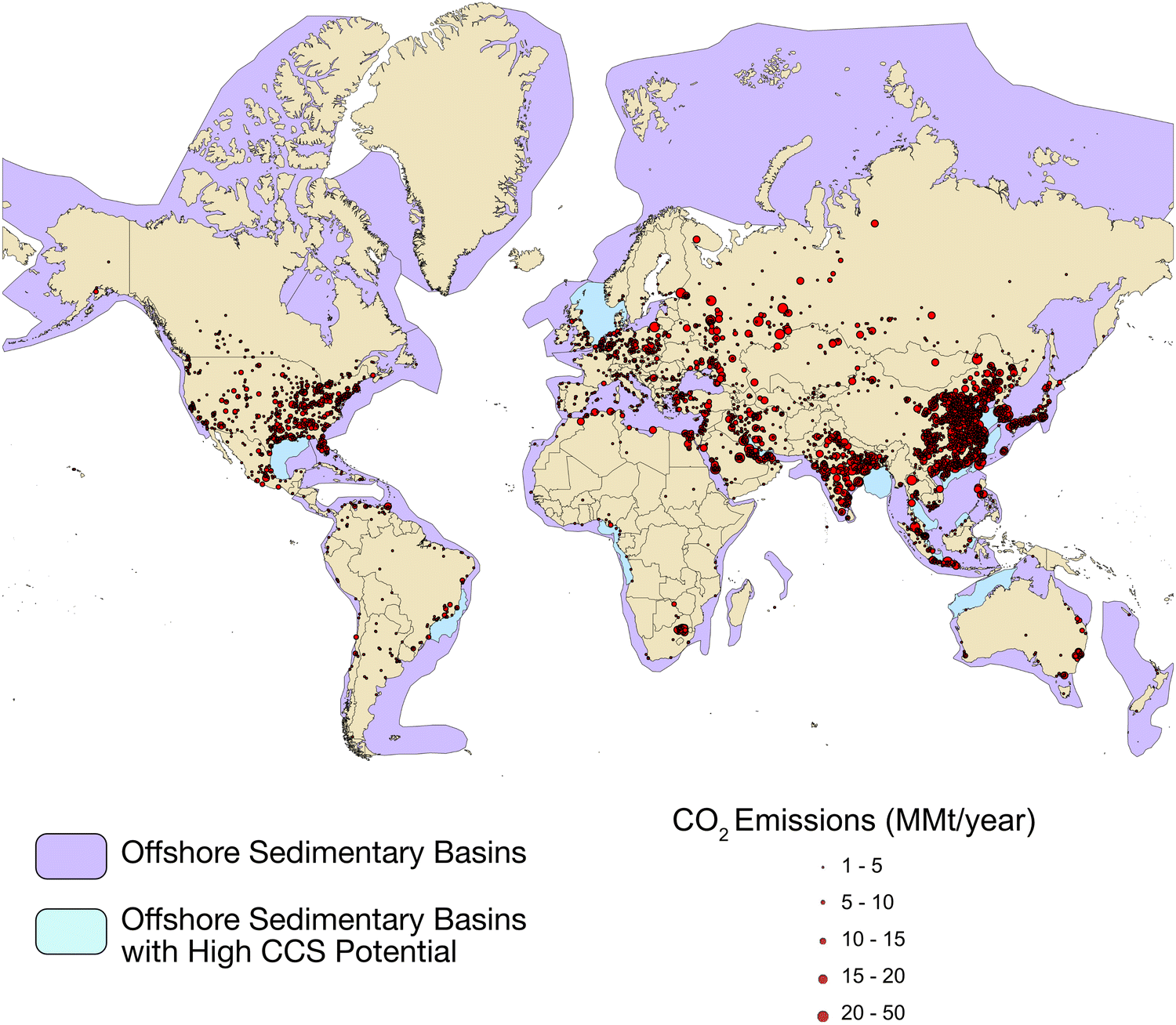 | ||
| Fig. 12 World map illustrating the proximity of major CO2 emissions to potential offshore saline storage sites. CO2 emissions data is from the emissions database for global atmospheric research (EDGAR) 2021 dataset.73 Global offshore sedimentary basins are shown in purple.71 Offshore sedimentary basins that we consider especially favorable for CCS through a combination of exploration, mature oil and gas development, and proximity to CO2 emission sources are shown in blue. | ||
Conclusions
This study implements ensemble simulation methods to evaluate the impact of spatially variable permeability on reservoir performance for CO2 storage in an offshore geologic setting. We conducted an ensemble simulation with fifty model realizations with highly heterogenous permeability structures. These methods are readily transferrable to CO2 reservoir assessment in offshore basins worldwide, and results from this modelling study offer generalized insights into reservoir performance characteristics when permeability is poorly constrained. For this model and simulation scenario, we find:1. Two zones where permeability distribution imposes substantial control over CO2 flow paths. In the region nearest the injection site, a relative permeability feedback emerges in which CO2 initially flows towards the regions of highest bulk permeability. This causes CO2 saturation to rise, thus increasing non-wetting phase permeability and allowing more CO2 to enter the region. As this phenomenon is observed both in our uncorrelated permeability models and past research with correlated models, this process appears to be independent of permeability correlation. In the far-field, results from this study suggest that mean (N = 50) flow paths generally converge on a concentric pattern around the injection well; however, the lateral extent of any individual CO2 plume will be highly dependent on far-field permeability. These results demonstrate the importance of predicting and characterizing both near-field and far-field permeability in a CO2 storage reservoir when planning CO2 storage and monitoring projects.
2. Temperature change is a potential early indicator for CO2 flow. A warming front from CO2 dissolution in water arrives hundreds of days prior to free phase CO2 arrival. Therefore, temperature monitoring above sealing layers may be an effective method for monitoring CO2 containment; however, we find that this result is more robust at longer radial distance from the injection well, which means longer time intervals are needed to identify a robust thermal signal.
3. In a fault-bounded system, 1 MMT per year CO2 injection for 10 years may drive sufficient fluid pressure to induce seismicity on optimally oriented, critically stressed faults. This suggests non-negligible risk of fault reactivation and potential breaching of sealing layers in storage systems containing faults; however, substantially more research is needed to understand the implications of pressure-induced geomechanics at reservoir scales.
To close, we note that the path to decarbonization is a monumental global challenge that requires rapid deployment of all commercially viable low carbon energy technologies. In this context, we hope that this study spurs additional interest and investment in offshore CCS technology because the geology appears favorable for CO2 storage and there are a number of offshore basins in close proximity to major CO2 sources.
Author contributions
L. W. K. is responsible for numerical simulations, analyses, and manuscript preparation. B. W. R. assisted with seismic interpretations and manuscript review. R. M. P. is responsible for study design, analyses, and manuscript review.Conflicts of interest
There are no conflicts to declare.Acknowledgements
The authors thank Dr. Philip Stauffer and one anonymous reviewer for insightful comments. This research was supported by the U.S. Department of Energy through the Southern States Energy Board SECARB Offshore project.Notes and references
- S. M. Benson and D. R. Cole, Elements, 2008, 4, 325–331 CrossRef CAS.
- P. Kelemen, S. M. Benson, H. Pilorge, P. Psarras and J. Wilcox, Front. Climate, 2019, 1, 9 CrossRef.
- S. Bachu, Prog. Energy Combust. Sci., 2008, 34, 254–273 CrossRef CAS.
- IPCC, Summary for Policymakers, Cambridge University Press, Cambridge, United Kingdom and New York, NY, USA, 2021 Search PubMed.
- S. D. Locker and A. C. Hine, Scenarios and Responses to Future Deep Oil Spills, Springer, Cham, 2020 DOI:10.1007/978-3-030-12963-7_4.
- U.S. Dept. of Energy National Energy Technology Laboratory (NETL), Carbon Storage Atlas, 5th edn, 2015.
- U.S. Environmental Protection Agency (EPA) Greenhouse Gas Reporting Program (GHGRP) Emissions by Location, https://www.epa.gov/ghgreporting/ghgrp-emissions-location, (March 2022).
- U.S. Dept. of Energy National Energy Technology Laboratory (NETL), Best Practices: Monitoring, Verification and Accounting (MVA) for Geologic Storage Projects, Revised Edition, Report DOE/NETL-2017/1847, 2017.
- R. S. Middleton and J. M. Bielicki, Energy Policy, 2009, 37, 1052–1060 CrossRef.
- R. S. Middleton, G. N. Keating, P. H. Stauffer, A. B. Jordan, H. S. Viswanathan, Q. J. Kang, K. W. Carey, M. L. M. E. J. Sullivan, S. P. Chu, R. Esposito and T. A. Meckel, Energy Environ. Sci., 2012, 5, 7328 RSC.
- D. Schulze-Makuch, D. Carlson, D. A. Cherkauer and P. Malik, Groundwater, 1999, 37, 904–919 CrossRef CAS.
- V. C. Tidwell and J. L. Wilson, SPE Reservoir Evaluation Eng., 2000, 3, 283–291 CrossRef CAS.
- H. Wu, N. Lubbers, H. S. Viswanathan and R. M. Pollyea, Appl. Energy, 2021, 287, 116580 CrossRef CAS.
- R. S. Jayne, H. Wu and R. M. Pollyea, Int. J. Greenhouse Gas Control, 2019, 83, 128–139 CrossRef CAS.
- A.-K. Furre, O. Eiken, A. Havard, J. N. Vevatne and A. F. Kiaer, Energy Proc., 2017, 114, 3916–3926 CrossRef CAS.
- R. A. Chadwick, P. Zweigel, U. Gregersen, G. A. Kirby, S. Holloway and P. N. Johannessen, Energy, 2004, 29, 1371–1381 CrossRef CAS.
- P. S. Ringrose, A. S. Mathieson, I. W. Wright, F. Selama, O. Hansen, R. Bissell, N. Saoula and J. Midgley, Energy Proc., 2013, 37, 6226–6236 CrossRef CAS.
- H. Deng, P. H. Stauffer, Z. Dai, Z. Jiao and R. C. Surdam, Int. J. Greenhouse Gas Control, 2012, 10, 397–418 CrossRef CAS.
- Z. Dai, P. H. Stauffer, J. W. Carey, R. S. Middleton, Z. Lu, J. F. Jacobs, K. Hnottavange-Telleen and L. H. Spangler, Environ. Sci. Technol., 2014, 48, 3601–4216 CrossRef PubMed.
- Z. Dai, Y. Zhang, J. Bielicki, M. A. Amooie, M. Zhang, C. Yang, Y. Zou, W. Ampomah, T. Xiao, W. Jia, R. Middleton, W. Zhang, Y. Sun, J. Moortgat, M. R. Soltanian and P. Stauffer, Appl. Energy, 2018, 225, 876–883 CrossRef CAS.
- R. M. Pollyea and J. P. Fairley, Hydrogeol. J., 2012, 20, 689–699 CrossRef CAS.
- R. M. Pollyea, J. P. Fairley, R. K. Podgorney and T. L. Mcling, Bull. Geological Soc. America, 2014, 126, 344–351 Search PubMed.
- O. Hansen, D. Gilding, B. Nazarian, B. Osdal, P. Ringrose, J.-B. Kristoffersen, O. Eiken and H. Hansen, Energy Proc., 2013, 37, 3565–3573 CrossRef CAS.
- L. W. Koehn, B. W. Romans and R. M. Pollyea, SEG/AAPG Second Int. Meeting Appl. Geosci. Energy, 2022, 547–551 Search PubMed.
- P. Zweigel, M. Hamborg, R. Arts, A. Lothe, Ø. Sylta and A. Tømmerås, presented in part at the Fifth International Conference on Greenhouse Gas Control Technologies, Cairns, Australia, 13-16 August, 2000.
- P. Ziemkiewicz, P. H. Stauffer, J. Sullivan-Graham, S. P. Chu, W. L. Bourcier, T. A. Buscheck, T. Carr, J. Donovan, Z. Jiao, L. Lin, L. Song and J. L. Wagoner, Int. J. Greenhouse Gas Control, 2016, 54, 538–556 CrossRef CAS.
- N. Heinemann, M. Wilkinson, G. E. Pickup, R. S. Haszeldine and N. A. Cutler, Int. J. Greenhouse Gas Control, 2012, 6, 210–219 CrossRef CAS.
- U.S. National Oceanic and Atmospheric Administration (NOAA) Gulf of Mexico Data Atlas, https://gulfatlas.noaa.gov/, (March 2023).
- U.S. National Archive of Marine Seismic Surveys: B-06-92-LA, https://walrus.wr.usgs.gov/namss/survey/b-06-92-la/, (October 2021).
- U.S. Bureau of Ocean Energy Management Atlas of Gulf of Mexico gas and oil sands data, https://www.data.boem.gov/Main/GandG.aspx, (October 2021).
- T. F. Hentz and H. Zeng, AAPG Bull., 2003, 87, 197–230 CrossRef CAS.
- RockWare, PetraSim User Manual, 2022 Search PubMed.
- J. Lu, D. L. Carr, R. H. Trevino, J.-L. T. Rhatigan and R. Fifariz, in Geological CO2 Sequestration Atlas of Miocene Strata, Offshore Texas State Waters, ed. R. H. Trevino and T. A. Meckel, The University of Texas at Austin, Bureau of Economic Geology, Austin, TX, 2017, pp. 14–25 Search PubMed.
- J. P. Fairley and J. J. Hinds, Geophys. Res. Lett., 2004, 31, L19502 CrossRef.
- M. T. V. Genuchten, Soil Sci. Soc. Am. J., 1980, 44, 892–898 CrossRef.
- Y. Jung, G. S. H. Pau, S. Finsterle and R. M. Pollyea, Comput. Geosci., 2017, 108, 2–7 CrossRef.
- R. M. Pollyea, Int. J. Greenhouse Gas Control, 2016, 46, 7–17 CrossRef CAS.
- N. Yoshida, J. S. Levine and P. H. Stauffer, Int. J. Greenhouse Gas Control, 2016, 49, 161–178 CrossRef CAS.
- H. Wu, R. S. Jayne and R. M. Pollyea, Greenhouse Gases: Sci. Technol., 2018, 8, 1039–1052 CrossRef CAS.
- D. B. Bennion and S. Bachu, presented in part at the 2006 SPE Technical Conference and Exhibition, San Antonio, TX, 2006.
- L. A. Burke, S. A. Kinney, R. F. Dubiel and J. K. Pitman, GCAGS, 2012, 1, 97–106 Search PubMed.
- D. Blackwell, M. Richards, Z. Frone, J. Batir, A. Ruzo, R. Dingwall and M. Williams, GRC Trans., 2011, 35, 1545–1550 Search PubMed.
- L. Pan, N. Spycher, C. Doughty and K. Pruess, Greenhouse Gases: Sci. Technol., 2017, 7, 313–327 CrossRef CAS.
- K. Pruess and N. Spycher, Energy Convers. Manage., 2007, 48, 1761–1767 CrossRef CAS.
- C. V. Deutsch and A. G. Journel, GSLIB: Geostatistical Software Library and User's Guide, Oxford University Press, 2 edn, 1997 Search PubMed.
- T. Onishi, M. C. Nguyen, J. W. Carey, B. Will, W. Zaluski, D. W. Bowen, B. C. Devault, A. Duguid, Q. Zhou, S. H. Fairweather, L. H. Spangler and P. H. Stauffer, Int. J. Greenhouse Gas Control, 2019, 81, 44–65 CrossRef CAS.
- M. C. Nguyen, M. Dejam, M. Fazelalavi, Y. Zhang, G. W. Gay, D. W. Bowen, L. H. Spangler, W. Zaluski and P. H. Stauffer, Int. J. Greenhouse Gas Control, 2021, 108, 103326 CrossRef CAS.
- J. Ennis-King, T. Dance, J. Xu, C. Boreham, B. Freifeld, C. Jenkins, L. Paterson, S. Sharma, L. Stalker and J. Underschultz, Energy Procedia, 2011, 4, 3494–3501 CrossRef.
- R. A. Chadwick and D. J. Noy, Greenhouse Gases: Sci. Technol., 2015, 5, 305–322 CrossRef CAS.
- R. S. Jayne, Y. Zhang and R. M. Pollyea, Geophys. Res. Lett., 2019, 46, 5879–5888 CrossRef CAS.
- W. S. Han, G. A. Stillman, M. Lu, C. Lu, B. J. McPherson and E. Park, J. Geophys. Res.: Solid Earth, 2010, B07209 Search PubMed.
- Z. Duan, R. Sun, C. Zhu and I. M. Chou, Mar. Chem., 2006, 131–139 CrossRef CAS.
- D. Koschel, J. Y. Coxam, L. Rodier and V. Majer, Fluid Phase Equilib., 2006, 107–120 CrossRef CAS.
- P. H. Stauffer, K. C. Lewis, J. S. Stein, B. J. Travis, P. Lichtner and G. Zyvoloski, Transp. Porous Media, 2014, 105, 471–485 CrossRef CAS.
- NIST, Thermophysical properties of fluid systems, https://webbook.nist.gov/chemistry/fluid/, (August 2023).
- W. L. Yeck, L. V. Block, C. K. Wood and V. M. King, Geophys. J. Int., 2014, 200, 322–336 CrossRef.
- R. M. Pollyea, N. Mohammadi, J. E. Taylor and M. C. Chapman, Geology, 2018, 46, 215–218 CrossRef.
- R. M. Pollyea, G. L. Konzen, C. R. Chambers, J. A. Pritchard, H. Wu and R. S. Jayne, Energy Environ. Sci., 2020, 13, 3014–3031 RSC.
- P. A. Reasenberg and R. W. Simpson, Science, 1992, 225, 1687–1690 CrossRef PubMed.
- K. M. Keranen, M. Weingarten, G. A. Abers, B. A. Bekins and S. Ge, Science, 2014, 345, 448–451 CrossRef CAS PubMed.
- R. M. Pollyea, Hydrogeol. J., 2020, 28, 795–903 CrossRef.
- R. M. Pollyea, M. C. Chapman, R. S. Jayne and H. Wu, Nat. Commun., 2019, 10, 3077 CrossRef PubMed.
- F. Cappa, Y. Guglielmi, C. Nussbaum, L. D. Barros and J. Birkholzer, Nat. Geosci., 2022, 15, 747–751 CrossRef CAS.
- M. G. Rowan, M. P. A. Jackson and B. D. Trudgill, AAPG Bull., 1999, 83, 1454–1484 CAS.
- T. A. Buscheck, J. M. Bielicki, J. A. White, Y. Sun, Y. Hao, W. L. Bourcier, S. A. Carroll and R. D. Aines, Int. J. Greenhouse Gas Control, 2016, 54, 499–512 CrossRef CAS.
- T. A. Buscheck, J. A. White, S. A. Carroll, J. M. Bielicki and R. D. Aines, Energy Environ. Sci., 2016, 9, 1504–1512 RSC.
- J. T. Birkholzer, A. Cihan and Q. Zhou, Int. J. Greenhouse Gas Control, 2012, 7, 168–180 CrossRef CAS.
- D. R. Harp, P. H. Stauffer, D. O’Malley, Z. Jiao, E. P. Egenolf, T. A. Miller, D. Martinez, K. A. Hunter, R. S. Middleton, J. M. Bielicki and R. Pawar, Int. J. Greenhouse Gas Control, 2017, 64, 43–59 CrossRef.
- K. Z. House, D. P. Schrag, C. F. Harvey and K. S. Lackner, Proc. Natl. Acad. Sci. U. S. A., 2006, 103, 12291–12295 CrossRef CAS PubMed.
- T. A. Meckel, R. Trevino and S. D. Hovorka, Energy Procedia, 2017, 114, 4728–4734 CrossRef.
- J. Bradshaw and T. Dance, Greenhouse Gas Control Technol., 2005, 7, 583–591 Search PubMed.
- P. S. Ringrose and T. A. Meckel, Sci. Rep., 2019, 9, 17944 CrossRef CAS PubMed.
- E.U. Emissions Database for Global Atmospheric Research (EDGAR), https://edgar.jrc.ec.europa.eu/dataset_ghg70, (March 2023).
Footnote |
| † Electronic supplementary information (ESI) available: Well log data used in model. See DOI: https://doi.org/10.1039/d3ya00317e |
| This journal is © The Royal Society of Chemistry 2023 |