
 Open Access Article
 This Open Access Article is licensed under a
 Creative Commons Attribution 3.0 Unported Licence
Application of deep learning to support peak picking during non-target high resolution mass spectrometry workflows in environmental research†
Kate
Mottershead
a and
Thomas H.
Miller
 *b
*b
aDepartment of Analytical, Environmental & Forensic Sciences, School of Population Health & Environmental Sciences, Faculty of Life Sciences and Medicine, King's College London, 150 Stamford Street, London SE1 9NH, UK
bCentre for Pollution Research & Policy, Department of Life Sciences, Brunel University London, Kingston Lane, Uxbridge, UB8 3PH, UK. E-mail: thomas.miller@brunel.ac.uk
First published on 19th April 2023
Abstract
With the advent of high-resolution mass spectrometry (HRMS), untargeted analytical approaches have become increasingly important across many different disciplines including environmental fields. However, analysing mass spectra produced by HRMS can be challenging due to the sensitivity of low abundance analytes, the complexity of sample matrices and the volume of data produced. This is further compounded by the challenge of using pre-processing algorithms to reliably extract useful information from the mass spectra whilst removing experimental artefacts and noise. It is essential that we investigate innovative technology to overcome these challenges and improve analysis in this data-rich area. The application of artificial intelligence to support data analysis in HRMS has a strong potential to improve current approaches and maximise the value of generated data. In this work, we investigated the application of a deep learning approach to classify MS peaks shortlisted by pre-processing workflows. The objective was to classify extracted ROIs into one of three classes to sort feature lists for downstream data interpretation. We developed and compared several convolutional neural networks (CNN) for peak classification using the Python library Keras. The optimized CNN demonstrated an overall accuracy of 85.5%, a sensitivity of 98.8% and selectively of 97.8%. The CNN approach rapidly and accurately classified peaks, reducing time and costs associated with manual curation of shortlisted features after peak picking. This will further support interpretation and understanding from this discovery-driven area of analytical science.
Environmental significanceEnvironmental fields are increasingly employing high-resolution mass spectrometry (HRMS) for non-target applications with methods often developed from areas such as metabolomics. A current challenge using HRMS is that data processing in non-target screening is complex and requires manual curation and checking by the user adding significant time and resource costs. To support data analysis in these areas it is important to investigate the use of innovative technologies such as Artificial Intelligence (AI) to overcome these bottlenecks. A deep learning model was developed using image classification to determine whether features extracted out from raw HRMS data could be reliably classified as a peak or not. The work demonstrated these models could rapidly classify peaks from images significantly reducing time and cost. |
1. Introduction
Mass spectrometry has long supported understanding for environmental research concerned with characterizing chemical mixtures in the environment, identifying transformation and/or degradation products, measuring kinetics of uptake and elimination and identification of toxins among many other applications.1 High resolution mass spectrometry (HRMS) coupled to liquid chromatography (LC) or gas chromatography (GC) is the basis of many studies that have demonstrated importance in clinical medicine, public health and epidemiology which are now emerging within the environmental space and include metabolomics, lipidomics and exposomics.2–6 The technique has typically three approaches including targeted, untargeted and suspect screening (i.e. semi-targeted). In targeted analysis compounds, or compound classes are determined and is often quantitative. However, targeted methods cover a relatively small proportion of compounds that must be known a priori preventing discovery of unknown compounds and can further result in analytical bias (i.e. the Matthew effect).7 Alternatively, untargeted mass spectrometry is a comprehensive approach that aims to detect all compounds present within a sample enabling discovery of novel compounds. HRMS produces signals, or peaks, described by the retention time (tR) and mass-to-charge ratio (m/z) that require annotation to enable interpretation of the data. Peaks can be matched to mass spectral libraries but annotation is limited by the availability of certified reference standards for confirmatory analysis. Moreover, for applications such as metabolomics, several thousand peaks can be detected in one sample which requires significant time to process to ensure extracted features are real signals.8Untargeted analysis generates a significant amount of data requiring extensive processing before data interpretation stages. The data processing referred to as pre-processing is used to generate a feature list (i.e. a list of m/z–tR pairs) that have been measured by the mass analyser. There are many approaches and algorithms used to extract this information and perform peak picking including vendor-specific software and freely available packages such as XCMS9 and MZmine.10 However, these algorithms are not without limitations and peak picking can often extract noise instead of a true signal (i.e. a peak).11,12 Therefore, feature lists can contain a large number of false positives. This can be reduced somewhat by appropriate optimization of parameter settings during peak picking but does not completely solve the issue. Furthermore, implementing more stringent parameter settings can also reduce the sensitivity for a true signal so that potentially important peaks are not extracted out of the raw data.13–15 To ensure that the signal is a true positive, feature lists must be manually inspected leading to a laborious process that is prone to human error.16
Different research groups have attempted to improve this situation by developing approaches to reduce false positives and improve quality control.14,16 A potential solution to significantly reduce the need for manual curation is through the application of artificial intelligence (AI). AI is the ‘cognitive ability’ demonstrated by machines and the field is further separated into machine learning (ML) and deep learning (DL) which enables machines to learn. The advantage of ML and DL is that they can model a process in a rapid, automated and reliable way. Furthermore, DL models, such as convolutional neural networks (CNNs), can be trained on visual data such as images. This approach can be utilised for untargeted analysis where feature lists require visual inspection and the extracted ion chromatograms can be exported as images. For example, a previous investigation by Melnikov et al. used a CNN to create an algorithm which is capable of peak classification and integration of raw LC-HRMS data.17 These early studies of DL applications for untargeted metabolomics data analysis show good potential for the use of AI in analytical science. With further advancements in accuracy and generalizability of models, the impact of AI in untargeted analysis has the potential to increase accuracy whilst decreasing the overhead and further support data interpretation.
The aim of this work was to demonstrate the applicability of CNNs for peak classification of regions of interest (ROIs) extracted from an untargeted LC-HRMS analysis. Feature lists (tR–m/z pairs) were extracted using XCMS in R. Several CNN models were applied and compared for their ability to categorise these features (i.e., ROIs) as true positives, false positives and those requiring further investigation. The optimised CNN was then applied to two external datasets to test the generalisability of the model to classify peaks from other HRMS datasets. The application of CNNs to identify peaks during untargeted workflows would provide an automated, data driven solution to support downstream data interpretation, saving significant time and costs.
2. Materials & methods
2.1. Data collection and processing
Raw LC-HRMS data was acquired in-house from a metabolomic study in which a freshwater invertebrate, Gammarus pulex, was exposed to different chemicals. Briefly, sample preparation involved a biphasic liquid extraction to extract metabolites into a polar and non-polar phase. The polar fraction was taken for analysis using an Exactive Orbitrap mass analyser with polarity switching coupled to a Vanquish LC system (ThermoFisher, Hemel Hempstead, UK). Separation was achieved using hydrophilic interaction liquid chromatography (HILIC) on a SeQuant ZIC pHILIC stationary phase (4.6 mm × 150 mm, 5 μM particle size, Merck, Hertfordshire, UK). Chromatographic run time was 25 min including a 5 min re-equilibration period to starting conditions. Mobile phase A was 20 mm ammonium carbonate and mobile phase B was acetonitrile. An in-house script in R (https://www.r-project.org/) using packages xcms and CAMERA was used for peak picking. The R script used a peak detection algorithm (CentWave) from XCMS and processed the raw MS data to generate a feature list of tR–m/z pairs. The peaking picking parameters were as follows; ppm = 10, peakwidth = 10 & 65, snthresh = 30, prefilter = 7 & 6000, mzCenterfun = wMean, integrate = 2, mzdiff = 0.002 and noise = 2000. The features, or ROIs, were scaled to unity and exported as extracted ion chromatograms saved in a .png format. From 120 samples, over 100![[thin space (1/6-em)]](https://www.rsc.org/images/entities/char_2009.gif) 000 ROI files were exported and 4000 images were randomly selected for manual curation into the training and test data.
000 ROI files were exported and 4000 images were randomly selected for manual curation into the training and test data.
The ROI files were labelled into three classes; files containing a true chromatographic peak(s) (Type I), files containing no identifiable chromatographic peak (Type II) or files that needed further investigation (Type III). Several criteria were applied during the manual labelling of the ROI files to ensure consistency and reproducibility (see ESI, Fig. S1†). Images were labelled with the class (i.e., Types I–III) against each file name in an excel spreadsheet and then a robot script was written and applied to append the class name to each of the ROI's file name.
2.2. Image pre-processing
All DL code was written in Python v3.8 (https://www.python.org/) using the open-source editing tool Jupyter Notebook (https://jupyter.org/). Keras (https://keras.io/), a neural network API from the open-source TensorFlow library (https://www.tensorflow.org/).The script first organises the data into train, validation and test subsets. The train and validation sets are used to develop and optimise the model parameters. The test set is then used to test the model classifications on new data not previously used in the model development to get a more robust estimate of model performance. The train set was given 2759 ROIs (70% of the data) split across the classes as 1290 Type I, 769 Type II and 700 Type III, the validation set contained 799 ROIs (20% of the data) split across the classes as 368 Type I, 231 Type II and 200 Type III, and finally the test set contained 442 ROIs (10% of the data) split across the classes as 185 Type I, 157 Type II and 100 Type III. The ROIs assigned to each class in each set was fixed. The ROI image files were pre-processed into an image data format (.png) that the Keras neural network could receive (e.g., png, jpeg, bmp, gif). Different pre-trained CNN models are available as applications online (https://keras.io/api/applications/), which were created externally on different image data types, and can be utilised in the pre-processing step. In the CNN models that were applied in this study, three different apps were used to provide the image pre-processing: VGG-16, Xception and MobileNet (see ESI, Fig. S2†).
2.3. Model development and optimisation
Three simple sequential models (Models A–C) were built first using a 2D convolution layer (Conv2D), a 2D max pooling layer (MaxPool2D) another Conv2D layer and MaxPool2D layer, a flatten layer and then a dense output layer. Layers here correspond to the internal architecture of the CNN model. The model was complied with the Adam optimizer, the learning rate was set to 0.001 and the loss function was set as categorical cross-entropy. Finally, the model was run over 10 epochs (rounds). The process was repeated 5 times for each pre-processing app each model with the highest validation accuracy and lowest variance selected. The test set was then run against this model and a confusion matrix was produced to represent the predicted class labels versus the true class labels.Three more complex, fine-tuned CNN models were then built using the pre-trained model applications from Keras: VGG16, Xception and MobileNet. In all cases the pre-trained models were downloaded and then modified and a dense output layer (with 3 outputs) was added. All models had different layer types (see ESI, Table S1†), The VGG16 model had 23 layers containing a mixture of Conv2D and MaxPool2D layers. The Xception model had 126 layers, containing; activation, separable convolutional, batch normal, Conv2D, MaxPool2D and used a global average pooling layer for the final layer. The MobileNet model, the least complex of the three models (4253864 parameters), contained 88 layers including Conv2D, Rectified Linear Unit, Depthwise Conv2D, batch normalization, zero padding and global average pooling layers. A variety of batch sizes, number of epochs, and learning rates were trialed across all models to assess the overfitting and underfitting of the models. Overfitting would mean increased sensitivity of the model to the train sets ROI image details, resulting in a negative impact on the performance of the model against other ROI images. This can be observed, whilst increasing parameters such as epochs, at the point when the accuracy of the model against the train set begins to improve at a faster rate than the accuracy of the validation set and this was used to assess overfitting of the models tested here. The final parameters were set to use the Adam optimizer, with a learning rate of 0.001, a batch-size of 50, a loss function of categorical cross-entropy, epochs set to 10 and each model trained twice. As with the simpler model, the test data were then run against the best of two models for each optimised pre-trained model and a confusion matrix was produced.
2.4. Model assessment
The best CNN model was selected and externally tested without retraining using two available datasets from the MetaboLights repository (https://www.ebi.ac.uk/metabolights/index). The first study applied a targeted HRMS method to determine 50 lipids from human plasma samples (Koulman et al., 2009, MTBLS4, https://www.ebi.ac.uk/metabolights/MTBLS4/descriptors). We used a targeted method to externally test and validate our model as these ROIs could be confirmed as true positives. The external dataset was downloaded and the same pre-processing workflow (i.e. peak picking) was applied as described above. In a second study that investigated metabolism of the sexual cycle of a marine diatom (Fiorini et al., 2020, MTBLS1714, https://www.ebi.ac.uk/metabolights/MTBLS1714/descriptors) we applied our pre-processing workflow to extract features from the available files and randomly split a small subset of the final feature list into 50 Type I ROIs and 50 type II ROIs to further test the model predictions. The peak picking here was not optimised but used values specified by the authors where possible19 (i.e. MZmine was used that had different parameters).In binary data classification, the reliability of a model typically includes measures of sensitivity and selectivity (eqn (1) and (2)).
 | (1) |
 | (2) |
3. Results & discussion
3.1. CNNs for peak picking in HRMS
Initially, three simple sequential models were trained using three different image pre-processing apps. Model A had the highest test set accuracy of 76.47%, but the lowest selectivity of the three models 0.857, Models B and C had the same test set accuracy of 76.24%, but model B had the highest selectivity of 0.915, and Model C had the highest sensitivity of 0.971 (Fig. 1 and Table 1). | ||
| Fig. 1 Confusion matrix of CNN: (i) Model A (ii) Model B (iii) Model C (iv) Model D (v) Model E (vi) Model F. The matrix represents the number of files predictively labelled by the CNN model as either Type I, Type II or Type III ROIs from the test data against the true label. Each matrix includes 442 ROIs: 185 Type I, 157 Type II and Type III. | ||
| CNN model | Pre-processing app (PPA)/pre-trained model (PTM) | Test set accuracy (%) | Sensitivity | Selectivity | Type III misclassification (%) |
|---|---|---|---|---|---|
| A | VGG16 (PPA) | 76.47 | 0.965 | 0.857 | 12.6 |
| B | MobileNet (PPA) | 76.24 | 0.964 | 0.915 | 16.4 |
| C | Xception (PPA) | 76.24 | 0.971 | 0.892 | 14.2 |
| D | VGG16 (PTM) | 83.03 | 0.988 | 0.977 | 14.0 |
| E | MobileNet (PTM) | 85.52 | 0.988 | 0.978 | 9.9 |
| F | Xception (PTM) | 84.84 | 0.994 | 0.971 | 8.8 |
| Melnikov et al. | — | 87.33 | 0.994 | 0.989 | 24.0 |
Following this the pre-trained models; VGG16 (D), MobileNet (E) and Xception (F) were downloaded in full and fine-tuned. These more complex models took a significantly longer time to train, thus training was repeated only once. The new models were assessed using the same criteria as previously. Model D and E had the same sensitivity of 0.988 compared to model F which had a better sensitivity of 0.994. However, Model E had the highest test accuracy of 85.52% and the highest selectivity of 0.978 (Table 1).
As mentioned before, the selectivity and sensitivity used to assess the models did not account for the Type III ROIs due to the ambiguity of this category. Although, comparisons of the model performance for the Type III class can be made from the percentage of ROIs predictively assigned to Type III that were not a true Type III (i.e. either a Type I or Type II). A higher number of ROIs predicted in the Type III class would mean an increased amount of time for manual investigation. Given this, Model E and F showed better performance, as misclassification of Type I or Type II ROIs into the Type III class was 9.9% and 8.8%, respectively. In comparison Model D had a misclassification of 14.0% for ROIs that were Type I or Type II (Table 1). Model E was selected as the best of the six developed models demonstrating the highest test set accuracy, high sensitivity, high selectivity and a low Type III misclassification.
The training of these models made use of available image pre-processing apps and, for models D-F, pre-trained CNNs were also applied. These models and their respective image pre-processing apps were developed from the ImageNet Large Scale Visual Recognition Challenge that has significantly advanced image recognition in DL approaches.20 The ImageNet dataset contains >1.3 M images covering 1000 object classes (e.g. cats & dogs, different lizard species and numbers). Although it is possible to create an image pre-processing app or a full model these methods are time consuming and typically yield worse accuracies than the use of pre-trained models. A paired two-tailed t-test showed that the test set accuracy of the simple models that were developed here (A–C) were statistically lower (p < 0.05) than the fine-tuned models (D–F) optimised from available pre-trained models. This transfer learning, where one model developed for a specific task is used as a starting point for a second task, is common within CNN approaches.21 By using pre-trained models, effort can instead be spent improving and fine-tuning models to be more accurate to a specific task. This follows one of the main concepts in AI of continuous improvement. However, the pre-trained models used in this study were trained on image data that is considerably different to extracted ion chromatograms, which in comparison are much simpler. Thus, the feature extraction by the CNN models may not be optimal for recognition of image features in the ROI files. If these pre-trained models had been developed using similar objects, then the CNN accuracy would potentially improve for this application.
3.2. External validation of the optimised CNN
Model E was externally tested using two published studies. The first used LC-HRMS to target 50 lipids in human plasma samples thus all extracted ion chromatograms were confirmed true positives.18 The second used both a targeted and untargeted approach to characterise metabolism in a marine diatom during its sexual phase of its life cycle. This also demonstrated that the CNN would generalize well to other HRMS datasets that targeted different metabolites and used different methodologies (i.e., chromatography and mass spectrometry methods). The accuracy of Model E for the Koulman et al., 2009 study was 100%. The CNN did not misclassify any of the ROI files extracted by the peak picking workflow. Of the 50 lipids targeted, only 47 were reported in the original publication and a further four were not detected in the previous study,18 leaving a total of 43 lipid targets. The peak picking workflow applied here using XCMS performed poorly for three of the lipids (Table 2) and extracted noise instead of the analytes. For these three features, Model E correctly classified them as Type II ROIs (i.e. containing no chromatographic peak). The remaining 40 lipid targets were correctly identified as Type I ROIs. In addition to simple predictions into separate class labels, the CNN model can also present predictions as a probability for each class (Fig. S3†). This enables further confidence when applying the model and assessing the peak classification of extracted features from HRMS datasets. The model showed high confidence in the prediction of the peak classes, with the probability of Type I ≥89% for most cases. Probability in prediction of Type I was lower for features 2, 4, 17 and 28 (75–85%) (Table 2).| Feature # | Lipid | Calc. m/z | Prediction (probability) | Class | ||
|---|---|---|---|---|---|---|
| Type I | Type II | Type III | ||||
| a Poor performance of the peak picking algorithm (XCMS). b Not detected in the original publication. | ||||||
| 1 | GPCho(14:0/0:0) | 468.3085 | 0.90 | 0.10 | 0.00 | Type I |
| 2 | GPEtn(18:1/0:0) | 480.3085 | 0.81 | 0.14 | 0.05 | Type I |
| 3 | GPCho(O-16:1) | 480.3449 | 0.99 | 0.01 | 0.00 | Type I |
| 4 | GPEtn(18:0/0:0) | 482.3241 | 0.80 | 0.20 | 0.00 | Type I |
| 5a | GPCho(O-16:0) | 482.3605 | 0.12 | 0.70 | 0.18 | Type II |
| 6 | GPCho(16:1/0:0) | 494.3241 | 0.99 | 0.01 | 0.00 | Type I |
| 7 | GPCho(16:0/0:0) | 496.3398 | 1.00 | 0.00 | 0.00 | Type I |
| 8 | GPEtn(20:4/0:0) | 502.2928 | 1.00 | 0.00 | 0.00 | Type I |
| 9a | GPCho(O-18:1) | 508.3762 | 0.10 | 0.90 | 0.00 | Type II |
| 10 | GPCho(18:3/0:0) | 518.3241 | 0.99 | 0.01 | 0.00 | Type I |
| 11 | GPCho(18:2/0:0) | 520.3398 | 0.90 | 0.10 | 0.00 | Type I |
| 12 | GPCho(18:1/0:0) | 522.3554 | 0.99 | 0.01 | 0.00 | Type I |
| 13 | GPCho(18:0/0:0) | 524.3711 | 0.99 | 0.01 | 0.00 | Type I |
| 14 | GPEtn(22:6/0:0) | 526.2938 | 0.99 | 0.01 | 0.00 | Type I |
| 15 | GPCho(20:5/0:0) | 542.3241 | 0.89 | 0.02 | 0.09 | Type I |
| 16 | GPCho(20:4/0:0) | 544.3398 | 0.92 | 0.08 | 0.00 | Type I |
| 17 | GPCho(20:3/0:0) | 546.3554 | 0.75 | 0.25 | 0.00 | Type I |
| 18 | GPCho(22:6/0:0) | 568.3398 | 0.97 | 0.03 | 0.00 | Type I |
| 19 | SM(d18:1/14:0) | 675.5436 | 0.92 | 0.07 | 0.00 | Type I |
| 20 | SM(d18:1/15:0) | 689.5592 | 0.94 | 0.03 | 0.03 | Type I |
| 21 | SM(d18:1/16:1) | 701.5592 | 1.00 | 0.00 | 0.00 | Type I |
| 22 | GPCho(O-34:3) | 742.5745 | 0.99 | 0.01 | 0.00 | Type I |
| 23b | GPCho(O-34:2) | 744.5902 | — | — | — | — |
| 24 | GPCho(34:4) | 754.5381 | 0.97 | 0.03 | 0.00 | Type I |
| 25 | GPCho(34:3) | 756.5538 | 0.94 | 0.06 | 0.00 | Type I |
| 26 | GPCho(34:2) | 758.5694 | 1.00 | 0.00 | 0.00 | Type I |
| 27 | GPCho(34:1) | 760.5851 | 1.00 | 0.00 | 0.00 | Type I |
| 28 | GPCho(O-36:6) | 764.5589 | 0.85 | 0.15 | 0.00 | Type I |
| 29 | GPCho(O-36:5) | 766.5745 | 0.93 | 0.07 | 0.00 | Type I |
| 30 | GPCho(O-36:3) | 770.6058 | 0.97 | 0.03 | 0.00 | Type I |
| 31 | GPCho(36:5) | 780.5538 | 1.00 | 0.00 | 0.00 | Type I |
| 32 | GPCho(36:4) | 782.5694 | 1.00 | 0.00 | 0.00 | Type I |
| 33 | GPCho(36:3) | 784.5851 | 0.98 | 0.00 | 0.00 | Type I |
| 34a | GPCho(36:2) | 786.6007 | 0.15 | 0.79 | 0.06 | Type II |
| 35b | GOCho(O-38:7) | 790.5745 | — | — | — | — |
| 36 | GPCho(O-38:6) | 792.5902 | 0.99 | 0.01 | 0.00 | Type I |
| 37 | GPCho(O-38:5) | 794.6058 | 1.00 | 0.00 | 0.00 | Type I |
| 38b | GPCho(O-38:4) | 796.6215 | — | — | — | — |
| 39 | GPCho(38:7) | 804.5538 | 1.00 | 0.00 | 0.00 | Type I |
| 40 | GPCho(38:6) | 806.5694 | 1.00 | 0.00 | 0.00 | Type I |
| 41 | GPCho(38:5) | 808.5851 | 1.00 | 0.00 | 0.00 | Type I |
| 42 | GPCho(38:4) | 810.6007 | 1.00 | 0.01 | 0.00 | Type I |
| 43 | GPCho(38:3) | 812.6164 | 1.00 | 0.00 | 0.00 | Type I |
| 44b | GPCho(O-40:6) | 820.6215 | — | — | — | — |
| 45 | GPCho(40:7) | 832.5851 | 1.00 | 0.00 | 0.00 | Type I |
| 46 | GPCho(40:6) | 834.6007 | 0.99 | 0.01 | 0.00 | Type I |
| 47 | GPCho(40:5) | 836.6164 | 1.00 | 0.00 | 0.00 | Type I |
In the second external test, the model was tested on the prediction performance of 50 Type I and 50 Type II ROIs that were manually assigned. This was to test the CNN on other data, methods and its confidence to classify true positives versus true negatives. The CNN demonstrated a classification accuracy of 94%, with a sensitivity of 0.900 and selectivity of 0.980. Suggesting that the model had lower predictive performance for determining true positives (i.e. Type I ROIs). The CNN correctly classified 49 of the Type II ROIs and 45 of the Type I ROIs. Misclassification included one Type II ROI as Type I, three Type I ROIs as Type II and two as Type III (Fig. 2). Two of the Type I ROIs misclassified as Type II contained multiple chromatographic peaks (Table S2 and Fig. S5†). Whilst the CNN could correctly classify ROIs with multiple peaks it showed lower performance for these types of ROIs. Multiple peaks can appear in a single ROI due to poor chromatographic resolution and potential structural isomers. However, these cases are typically few in number and with further training on these specific cases the model could be improved the image classification on multi-peak ROIs.
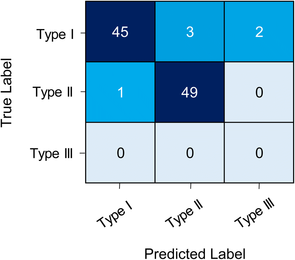 | ||
| Fig. 2 Confusion matrix of CNN tested on ROIs extracted from Fiorini et al., 2020. The matrix represents the number of files predictively labelled by the CNN model as either Type I, Type II or Type III ROIs from the test data against the true label. | ||
The lower prediction probability corresponded to features that had more than one peak present in the image file or was a narrow eluting peak (<10 s). The CNN model trained on ROI images in the present study, used a chromatography method that had wider eluting peaks (typically >20 s) due to the column dimensions and method parameters. Therefore, for these cases it is likely that Model E had a lower predictive confidence as it classified peaks outside of the data it was trained on. Nevertheless, the utility of model E was well demonstrated as it was tested on data generated from different analytical methodologies analysing different classes of metabolites with ROIs that varied considerably in terms of peak shape, number of points per peak and peak width. Furthermore, the model classification was not impacted by the retention window used whether it was for the full chromatographic run, a constant window either side of the signal or only the signal from the extracted ion chromatogram. The number of training cases was relatively low with <1000 cases for two of the classes (Type II and Type III). As a rule of thumb, training of CNNs for image classification need ∼1000 cases per class to ensure good model performance. Whilst accuracy for this specific external test was perfect, it is likely that with a larger dataset containing thousands of features the prediction will be closer to the internal test set accuracy (85.52%). Further model improvements could be made by using different training cases from several analytical methods, a larger number of ROI training cases for each class and further fine-tuning of CNN parameters. Nevertheless, the model presented here has demonstrated high accuracy on three datasets from three different analytical methods.
3.3. Comparison to Melnikov et al. CNN model performance
The approach used in this study was similar to the work presented by Melnikov et al. including ROI classification into three classes, ROI images scaled to unity at maximum and ROI dataset size 4000 images split across three classes.17 However, in our approach ROIs were extracted as images and the model was used for image classification. The benefit of this approach is that our model could be applied to established data processing workflows irrespective of tools used provided the ROIs can be exported as an image file. We also use the concept of transfer learning where pre-trained models can be utilised reducing the time needed for development and that this model can be applied to any HRMS data provided the feature lists can be exported as images. We compared the performance of the CNNs in this study with the CNN developed by Melnikov et al. From the reported data the accuracy, sensitivity and selectivity were calculated (Table 1). The Melnikov et al. CNN had a test set accuracy of 87.33%, a sensitivity of 0.994 and a selectivity of 0.989.17 When comparing this to the in-house Model E, the Melnikov et al. model had a higher test set accuracy (+1.81%), a higher selectivity (+0.011), and a similar sensitivity (+0.006). However, the Melnikov et al. model assigned a much higher percentage of ROIs (24.4%) to the Type III class. It is important to highlight that multiple approaches and models are being developed to support data-driven tools in nontarget mass spectrometry. For example, tools have also been developed that can evaluate the raw signal extracted from feature extraction tools (NeatMS22) and toolboxes that can support feature extraction and data visualization (MStractor23). This area is rapidly developing and will drive important downstream discovery during data interpretation stages.The ambiguous nature of this data makes assessing model performance difficult, especially when comparing models that have been trained on different image data to MS ROIs. Melnikov et al. noted that ROI classification was particularly difficult for those ROIs that required further investigation and peaks that were noisy and of low intensity.17 Therefore, depending on the user assigning the data, the process can be prone to subjective classification. By incorporating simple steps in the manual assignment stage, the labelling process is more transparent and reproducible. Several criteria (Fig. S1†) were used to assign ROIs into the respective classes to improve model robustness and reproducibility which can be challenging in ML and DL fields. For example, signal intensity and the baseline noise are important in assessing whether a ROI contains a true positive (i.e. a peak). Similarly, the tR of a peak can also give an indication of whether the ROI is a true positive or not. Early eluting peaks in the void can be attributed to unretained analytes or different types of contamination such as that arising from carry-over. Furthermore, CNNs can handle multiple input data types including text, numerical and image data. This numerical data could be appended to a fully connected layer at the end of the model and include multiple parameters relating to tR, intensity, baseline noise, peak asymmetry and peak width to further improve model classification of ROIs.24 Nevertheless, these studies demonstrate the applicability of image classification in DL to support data analysis in untargeted mass spectrometry. With further improvements, the integration of DL approaches into these data-intensive workflows will significantly reduce resource use associated with time and costs.
3.4. AI to support data-driven science in environmental research
AI fields including DL and ML are still early in their application within environmental research, but the potential benefit of this technology has been recognised in multiple areas.2,25–28 In the present study, image classification was demonstrated to show high accuracy, sensitivity and selectivity reducing the need for manual investigation of ROIs during pre-processing stages, that would improve data analysis for investigations using non-target HRMS. Indeed, this analytical approach is becoming more widely used in areas such as environmental toxicology where metabolomics, lipidomics and exposomics are supporting discovery-driven research to understand mechanisms of toxicological responses across different species29 and fully characterise chemical exposure in the environment.28,30A challenge in these areas, using these techniques is in part due to the complexity and scale of the data,2,30 thus automated, rapid and accurate approaches will be vital for our understanding to keep pace with the volume of data being generated in environmental research. Furthermore, predictive tools can support toolbox development for specific approaches. For example, ML has been demonstrated to accurately predict tR across multiple environmental matrices, collision cross section in ion mobility spectrometry and to support identification and annotation of compounds during non-target HRMS.28,31–33 These predictive models would complement the CNN developed here to improve annotation of unknown compounds. Moreover, the advantage of HRMS enables retrospective analysis to improve current knowledge related to exposure and risk.34
The use of DL and ML is not without challenge. There is a critical need for improved standards surrounding reporting, data sharing, and model accessibility when concerning DL and ML research.35,36 Additionally, models and tools developed are often not maintained so the use of these become limited and are often short-lived.37 Principles such as findability, accessibility, interoperability, and reuse of digital assets38 and guidance put forward by NeurIPS35 are beginning to address the issue. Improving these standards will be necessary to ensure that the well-known ‘reproducibility crisis’ does not extend to DL and ML applications.
Overall, the application of image recognition for untargeted mass spectrometry showed a good potential to improve the speed and accuracy of peak picking and compound annotation in complex matrices analysed by untargeted HRMS. These types of approaches will complement strategies aimed at improving feature detection and annotation that include increasing number of replicates, better quality assurance and quality control and improvement in peak picking algorithms. The model will be most beneficial in situations that have a low number of biological replicates, peak picking parameters have not been optimised or where several thousand features have been extracted. There is no single solution but by developing these models, researchers have the option available for sophisticated post-processing tools to support downstream data processing and interpretation. The biggest investment in time in these approaches is the training of the network which in this application took approximately 4 weeks to train and develop 21 models (five versions of each of the three simple sequential models, and two versions of each of the three complex models). However, once the model has been developed it can be applied to any dataset as demonstrated here. Furthermore, running the model takes seconds to predict for hundreds of ROIs without the need for manual inspection. This would save costs associated with this time-consuming stage and further support downstream data interpretation. Moreover, AI should be further explored and applied to new avenues across all areas of environmental research to fully understand the potential benefits of this technology.
Conflicts of interest
There are no conflicts of interest to declare.Acknowledgements
Part of this work was submitted as a postgraduate research project dissertation by KM based at King's College London.References
- F. Hernández, J. V. Sancho, M. Ibáñez, E. Abad, T. Portolés and L. Mattioli, Anal. Bioanal. Chem., 2012, 403, 1251–1264 CrossRef PubMed.
- M. Ljoncheva, T. Stepišnik, S. Džeroski and T. Kosjek, Trends Environ. Anal. Chem., 2020, 28, e00099 CrossRef CAS.
- Q. Fu, A. Scheidegger, E. Laczko and J. Hollender, Environ. Sci. Technol., 2021, 55(12), 7920–7929 CrossRef CAS PubMed.
- J. G. Bundy, M. P. Davey and M. R. Viant, Metabolomics, 2009, 5, 3–21 CrossRef CAS.
- R. Al-Salhi, A. Abdul-Sada, A. Lange, C. R. Tyler and E. M. Hill, Environ. Sci. Technol., 2012, 46(16), 9080–9088 CrossRef CAS PubMed.
- A. David, A. Lange, A. Abdul-Sada, C. R. Tyler and E. M. Hill, Environ. Sci. Technol., 2017, 51(1), 616–624 CrossRef CAS PubMed.
- C. G. Daughton, Sci. Total Environ., 2014, 466–467, 315–325 CrossRef CAS PubMed.
- W. B. Dunn, A. Erban, R. J. M. Weber, D. J. Creek, M. Brown, R. Breitling, T. Hankemeier, R. Goodacre, S. Neumann, J. Kopka and M. R. Viant, Metabolomics, 2013, 9, 44–66 CrossRef CAS.
- C. A. Smith, E. J. Want, G. O'Maille, R. Abagyan and G. Siuzdak, Anal. Chem., 2006, 78(3), 779–787 CrossRef CAS PubMed.
- T. Pluskal, S. Castillo, A. Villar-Briones and M. Orešič, BMC Bioinf., 2010, 11(1), 1–11 CrossRef PubMed.
- J. B. Coble and C. G. Fraga, J. Chromatogr. A, 2014, 1358, 155–164 CrossRef CAS PubMed.
- O. D. Myers, S. J. Sumner, S. Li, S. Barnes and X. Du, Anal. Chem., 2017, 89(17), 8689–8695 CrossRef CAS PubMed.
- M. Eliasson, S. Rännar, R. Madsen, M. A. Donten, E. Marsden-Edwards, T. Moritz, J. P. Shockcor, E. Johansson and J. Trygg, Anal. Chem., 2012, 84(15), 6869–6876 CrossRef CAS PubMed.
- B. C. DeFelice, S. S. Mehta, S. Samra, T. Čajka, B. Wancewicz and J. F. Fahrmann, et al. , Anal. Chem., 2017, 89(6), 3250–3255 CrossRef CAS PubMed.
- J. Guo and T. Huan, Anal. Chim. Acta, 2020, 1137, 37–46 CrossRef CAS PubMed.
- S. Kutuzova, P. Colaianni, H. Röst, T. Sachsenberg, O. Alka, O. Kohlbacher, B. Burla, F. Torta, L. Schrübbers, M. Kristensen, L. Nielsen, M. J. Herrgård and D. McCloskey, Anal. Chem., 2020, 92(24), 15968–15974 CrossRef CAS PubMed.
- A. D. Melnikov, Y. P. Tsentalovich and V. V. Yanshole, Anal. Chem., 2020, 92(1), 588–592 CrossRef CAS PubMed.
- A. Koulman, G. Woffendin, V. K. Narayana, H. Welchman, C. Crone and D. A. Volmer, Rapid Commun. Mass Spectrom., 2009, 23(10), 1411–1418 CrossRef CAS PubMed.
- F. Fiorini, C. Borgonuovo, M. I. Ferrante and M. Brönstrup, Mar. Drugs, 2020, 18(6), 313 CrossRef CAS PubMed.
- J. Deng, W. Dong, R. Socher, L. J. Li, K. Li and F.-F. Li, ImageNet: A Large-Scale Hierarchical Image Database, 2009 IEEE Conference on Computer Vision and Pattern Recognition (CVPR), Institute of Electrical and Electronics Engineers (IEEE), 2009, pp. 248–55 Search PubMed.
- D. Han, Q. Liu and W. Fan, Expert Syst. Appl., 2018, 95, 43–56 CrossRef.
- Y. Gloaguen, J. A. Kirwan and D. Beule, Anal. Chem., 2022, 2022, 4930–4937 CrossRef PubMed.
- L. Nicolotti, J. Hack, M. Herderich and N. Lloyd, Metabolites, 2021, 11(8), 492 CrossRef CAS PubMed.
- J. Zhang, E. Gonzalez, T. Hestilow, W. Haskins and Y. Huang, Curr. Genomics, 2009, 10(6), 388–401 CrossRef CAS PubMed.
- X. Ren, Z. Mi and P. G. Georgopoulos, Environ. Int., 2020, 142, 105827 CrossRef CAS PubMed.
- P. Hou, O. Jolliet, J. Zhu and M. Xu, Environ. Int., 2020, 135, 105393 CrossRef CAS PubMed.
- S. F. Owen and J. R. Snape, The Era of Artificial Intelligence, Machine Learning, and Data Science in the Pharmaceutical Industry, Elsevier, 2021, pp. 217–235 Search PubMed.
- L. Bijlsma, M. H. G. Berntssen and S. Merel, Anal. Chem., 2019, 91(9), 6321–6328 CrossRef CAS PubMed.
- C. Rivetti, T. E. H. Allen, J. B. Brown, E. Butler, P. L. Carmichael, J. K. Colbourne, M. Dent, F. Falciani, L. Gunnarsson, S. Gutsell, J. A. Harrill, G. Hodges, P. Jennings, R. Judson, A. Kienzler, L. Margiotta-Casaluci, I. Muller, S. F. Owen, C. Rendal, P. J. Russell, S. Scott, F. Sewell, I. Shah, M. R. Viant, C. Westmoreland, A. White and B. Campos, Toxicol. in Vitro, 2020, 62, 104692 CrossRef PubMed.
- F. Hernández, J. Bakker, L. Bijlsma, J. de Boer, A. M. Botero-Coy, Y. Bruinen de Bruin, S. Fischer, J. Hollender, B. Kasprzyk-Hordern, M. Lamoree, F. J. López, T. L. ter Laak, J. A. van Leerdam, J. V. Sancho, E. L. Schymanski, P. de Voogt and E. A. Hogendoorn, Chemosphere, 2019, 222, 564–583 CrossRef PubMed.
- R. Bade, L. Bijlsma, T. H. Miller, L. P. Barron, J. V. Sancho and F. Hernández, Sci. Total Environ., 2015, 538, 934–941 CrossRef CAS PubMed.
- R. Aalizadeh, N. A. Alygizakis, E. L. Schymanski, M. Krauss, T. Schulze and M. Ibáñez, et al. , Anal. Chem., 2021, 93(33), 11601–11611 CrossRef CAS PubMed.
- A. Celma, R. Bade, J. V. Sancho, F. Hernandez, M. Humphries and L. Bijlsma, J. Chem. Inf. Model., 2022, 62(22), 5425–5434 CrossRef CAS PubMed.
- N. Creusot, C. Casado-Martinez, A. Chiaia-Hernandez, K. Kiefer, B. J. D. Ferrari, Q. Fu, N. Munz, C. Stamm, A. Tlili and J. Hollender, Environ. Int., 2020, 139, 105708 CrossRef CAS PubMed.
- J. Pineau, P. Vincent-Lamarre, K. Sinha, V. Larivière, A. Beygelzimer, F. d'Alché-Buc, E. Fox, and H. Larochelle, Improving Reproducibility in Machine Learning Research, NeurIPS, 2020 Search PubMed.
- T. Hernandez-Boussard, S. Bozkurt, J. P. A. Ioannidis and N. H. Shah, J. Am. Med. Inf. Assoc., 2020, 27, 2011–2015 CrossRef PubMed.
- A. Stupple, D. Singerman and L. A. Celi, npj Digit. Med., 2019, 2(1), 1–3 CrossRef PubMed.
- M. D. Wilkinson, M. Dumontier, IjJ. Aalbersberg, G. Appleton, M. Axton, A. Baak, N. Blomberg, J. W. Boiten, L. B. da Silva Santos, P. E. Bourne, J. Bouwman, A. J. Brookes, T. Clark, M. Crosas, I. Dilo, O. Dumon, S. Edmunds, A. Finkers RGonzales-Beltran, A. J. G. Gray, P. Groth, C. Goble, J. S. Grethe, J. Heringa, P. A. C. t Hoen, R. Hooft, T. Kuhn, R. Kok, J. Kok, S. J. Lusher, M. E. Martone, A. Mons, A. L. Packer, B. Persson, P. Rocca-Serra, M. Roos, R. van Schaik, S. A. Sansone, E. Schultes, T. Sengstag, T. Slater, G. Strawn, M. A. Swertz, M. Thompson, J. Van Der Lei, E. Van Mulligen, J. Velterop, A. Waagmeester, P. Wittenberg, K. Wolstencroft, J. Zhao and B. Mons, Sci. Data, 2016, 3(1), 1–9 Search PubMed.
Footnote |
| † Electronic supplementary information (ESI) available: Supplementary information; manual labelling criteria (Fig. S1), example CNN feature extraction of image files (Fig. S2), example predictions of ROI images using the optimised model (Fig. S3 and S4), architecture of CNN models (Table S1) and misclassification cases of external test from Fiorini et al., 2020 (Table S2 and Fig. S5). See DOI: https://doi.org/10.1039/d3va00005b |
| This journal is © The Royal Society of Chemistry 2023 |