
 Open Access Article
 This Open Access Article is licensed under a
 Creative Commons Attribution 3.0 Unported Licence
Understanding the electronic structure of Y2Ti2O5S2 for green hydrogen production: a hybrid-DFT and GW study†
Katarina
Brlec
 ,
Christopher N.
Savory
and
David O.
Scanlon
*
,
Christopher N.
Savory
and
David O.
Scanlon
*
Department of Chemistry and Thomas Young Centre, University College London, London, UK. E-mail: d.scanlon@ucl.ac.uk
First published on 20th July 2023
Abstract
Utilising photocatalytic water splitting to produce green hydrogen is the key to reducing the carbon footprint of this crucial chemical feedstock. In this study, density functional theory (DFT) is employed to gain insights into the photocatalytic performance of an up-and-coming photocatalyst Y2Ti2O5S2 from first principles. Eleven non-polar clean surfaces are evaluated at the generalised gradient approximation level to obtain a plate-like Wulff shape that agrees well with the experimental data. The (001), (101) and (211) surfaces are considered further at hybrid-DFT level to determine their band alignments with respect to vacuum. The large band offset between the basal (001) and side (101) and (211) surfaces confirms experimentally observed spatial separation of hydrogen and oxygen evolution facets. Furthermore, relevant optoelectronic bulk properties were established using a combination of hybrid-DFT and many-body perturbation theory. The optical absorption of Y2Ti2O5S2 weakly onsets due to dipole–forbidden transitions, and hybrid Wannier–Mott/Frenkel excitonic behaviour is predicted to occur due to the two-dimensional electronic structure, with an exciton binding energy of 0.4 eV.
Hydrogen is often advertised as a green and clean fuel of the future, but it already is an important chemical feedstock. Worldwide, 96% of hydrogen is used in the chemical industry, mostly in production of ammonia fertilisers and hydrocarbon refining.1 However, despite its status as the most abundant substance in the universe, it is very scarce in its most useful H2 diatomic form on Earth, where it exists primarily in water, hydrocarbons and other organic matter.2,3 Hydrocarbons have been traditionally used in production of hydrogen, with coal gasification and steam methane reforming among the most popular methods. Both are highly energy-intensive and emit large quantities of COx gases (even when accounting for the proposed use of carbon capture), which is clearly unsustainable long-term.4,5
A clear alternative to hydrocarbon reforming lies in the other major source of hydrogen – water. In 1972, Honda and Fujishima discovered that hydrogen can be produced by water electrolysis using ultraviolet (UV) light shone on a TiO2 electrode, popularising the idea of photocatalysis.6 TiO2 has since become one of the most studied photocatalytic materials due to its high photocorrosive stability, ease of manufacture and non-toxicity.7–9 However, because of its wide band gap (3.2 eV) titania can only absorb UV light, which only comprises less than 5% of the entire incident light on Earth.10
To strike the balance between absorption of a wide light spectrum and satisfying the thermodynamic and kinetic demands of water splitting, 1.8–2.2 eV has been identified as the ideal band gap range for photocatalysis.11 While exceptionally stable in water, metal oxides suffer from low-lying O 2p states that push the valence band maximum down in energy, opening the band gap too wide. Sulphides, on the other hand, contain S 3p states that are higher in energy which close the band gap substantially without altering the conduction band edge. Unfortunately, sulphides tend to self-oxidise and photocorrode in a water medium, which makes them unsuitable as photocatalysts.12 However, the photocorrosion stability of oxides and favourable electronic structure of sulphides can be combined in mixed-anion oxysulphides.
The family of cation-deficient Ruddlesden-Popper Ln2Ti2O5S2 (Ln = Y, Nd, Sm, Gd, Tb, Dy, Ho and Er) compounds exhibit this behaviour with measured optical band gaps in the 1.8–2.2 eV.13,14 Sm2Ti2O5S2, Gd2Ti2O5S2 and Tb2Ti2O5S2 have been identified as promising photocatalysts for water splitting.15 All three compounds exhibit rates of H2 and O2 evolution of about 20 μmol h−1 under visible light in the presence of sacrificial electron donors and acceptors.15 Y2Ti2O5S2 demonstrated simultaneous stoichiometric production of H2 and O2 when loaded with Rh/Cr2O3 and IrO2 as hydrogen and oxygen evolution co-catalysts, respectively, achieving rates of about 2.5 μmol h−1 and 1.25 μmol h−1, resulting in an apparent quantum yield (AQY) of 2.3% under UV light.16 Higher evolution rates of were 80 μmol h−1 (H2) and 40 μmol h−1 (O2) achieved when the co-catalysts were loaded and tested as separate half-reactions, so Y2Ti2O5S2 performs better compared to its lanthanide counterparts. More recently an improved AQY for oxygen evolution of 6.3% under 420 nm light irradiation was reported with Co3O4 co-catalyst loading.17
With an experimental band gap of 1.9 eV, predicted suitable band alignment for water redox and calculated low hole and electron effective masses of 0.5 me in the in-plane direction, Y2Ti2O5S2 indeed has all the indicators of a promising earth-abundant photocatalyst.16,18 While several computational studies have focused on the properties of the bulk Y2Ti2O5S2, this study aims to unveil the surface properties using state-of-the-art computational methodology.18,19 In particular, this study explores surface behaviour and energetics during relaxations, and how that relates to the band edge positions of the surfaces. Additionally many-body perturbation theory calculations are performed to calculate bulk optoelectronic properties, including the exciton binding energy, to support our hybrid DFT calculations and explore the optical behaviour of the system.
1 Computational methodology
All density functional theory (DFT) calculations were performed with the Vienna Ab initio Simulation Package (VASP), using the recommended projector-augmented wave (PAW) potentials to simulate the core and valence electrons.20–23 The same converged plane wave energy cutoff (480 eV) and k-point meshes (5 × 5 × 5 for primitive, 5 × 5 × 1 for conventional) were used as in a previous study.18 The crystal structure (Fig. 1a) obtained from Materials Project was relaxed into the ground state using the generalised-gradient approximation (GGA) Perdew–Burke–Ernzerhof functional revised for solids (PBEsol) and the hybrid-DFT Heyd–Scuseria–Ernzerhof (HSE06) functional.24–26 The conventional unit cell was relaxed with no constraints on unit cell shape and volume, until the maximum force on any atom did not exceed 0.01 eV Å−1, using a higher energy cutoff (620 eV) to account for Pulay stress.27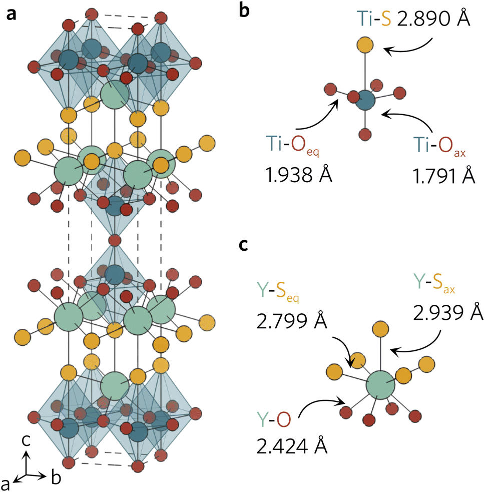 | ||
| Fig. 1 (a) Conventional unit cell of Y2Ti2O5S2 and local bonding environments of the TiO5S octahedra (b) and YO4S5 motifs (c) as calculated with HSE06. The atom colours are as follows: Y = light green, Ti = dark blue, S = yellow, O = red. The unit cell is represented with a dashed line. Plotted with VESTA.28 | ||
Because VASP cannot restrain the periodicity into just two dimensions, the slab model was employed herein to study the surface properties. The surfaxe package was used to cleave the slabs, calculate the parameters used in convergence testing and perform the relevant analyses.29 All non-polar, symmetric slabs up to a maximum Miller index of two were cleaved from the relaxed conventional unit cell.
To ensure the slabs were an accurate representation of the bulk and surfaces, extensive convergence testing to determine the minimal slab size required was conducted. For each of the Miller indices, the positions of atoms in the surface slabs with slab thicknesses ranging 10 to 50 Å were relaxed with PBEsol, while the unit cell shape and size was kept consistent. The average (arithmetic mean) bond distance change with respect to the atom's position in c-direction was used to ensure the bulk-like region was sufficiently large. If the average bond length close to the centre of the slab was close to the bond length of the same character in the bulk, then the slab was deemed to be sufficiently thick. The surface energy was also converged against slab thickness, where a criterion of 0.02 J m−2 was used to check convergence. Lastly, vacuum size was chosen to be 20 Å as this was the minimum thickness at which the planar potential was flat across all Miller indices.
For calculation of the band alignment of surfaces, the slabs were cleaved from the HSE06-relaxed bulk conventional unit cell. The atomic positions were then relaxed with HSE06 using the same force criterion as before, with constraints on unit cell shape and volume. This was done as hybrid functionals offer a better description of the electronic structure compared to GGA functionals, so the band alignment presented is more accurate.
Finally, the bulk effective charge carrier masses, dielectric constant and optical absorption spectrum discussed here were calculated as a part of a previous study.18
To assess the character of the exciton behaviour in Y2Ti2O5S2, many-body quasiparticle electronic structures and optical spectra were calculated within the Questaal package30 through the quasiparticle self-consistent GW (QSGW) method.31 Questaal utilises a full-potential linear muffin-tin orbital basis: augmentation sphere radii (in atomic units) of 2.80, 2.10, 2.49 and 1.52 were used for Y, Ti, S and O atoms respectively, with automatically generated interstitial smooth Hankel functions and an l-cutoff of 4 used for all atoms. Local orbitals were necessary to include the Ti 3p and Y 4p within the valence electrons. A GW k-mesh of 5 × 5 × 5 and interstitial G-vector cutoff of  were found to converge the quasiparticle gap to within 10 meV, with a 7 × 7 × 7 k-mesh used to obtain the initial PBE exchange–correlation potential. QSGW, which tends to demonstrate excellent agreement with experimental band gaps for s–p dominated semiconductors, overestimates band gaps systematically due to the usage of the Random Phase Approximation (RPA) – this can be improved by including ladder diagrams, which can describe the additional contribution by explicit two-particle electron–hole interaction to the screened Coulomb W;32 these can be obtained via the Bethe–Salpeter equation (BSE), and their additional to QSGW has lead to exceptional accuracy with respect to experimental band gaps in previous cases.33–35 The inclusion of these effects within a self-consistent calculation of the self-energy is here denoted QSGŴ, and within the explicit solution of optical transitions, to obtain excitonic features, QSGŴ + BSE (without, QSGŴ + RPA). Both QSGW and subsequent QSGŴ self-consistent cycles were iterated until the root-mean-square change in the self-energy was below 1 × 10⁻⁵. In the solution of the BSE, 8 valence and 8 conduction bands were used, with a k-mesh of 7 × 7 × 7 used for the optical spectrum, which ensured the dielectric constant (q → 0) was converged to within 0.01.
2 Results and discussion
The relaxed conventional unit cell can be seen in Fig. 1, together with the TiO5S and YO4S5 units. Compared to the experimental structure by Hyett et al.36 (I4/mmm, a = 3.770 Å, c = 22.806 Å), the volume of the unit cell decreased by 1.3% (PBEsol; I4/mmm, a = 3.755 Å, c = 22.682 Å) and 0.5% (HSE06; I4/mmm, a = 3.756 Å, c = 22.871 Å). The calculated lattice parameters clearly agree well with the experimental data, with slight differences between the two functionals in the out-of-plane c parameter.The larger volume decrease in the PBEsol-relaxed structure can be predominantly attributed to the shortening of Ti–S (−0.021 Å) and Y–Sax (−0.048 Å), whereas the bond distances were elongated by 0.022 Å and 0.017 Å in the HSE06 structure (see Table 1). For the interested reader, a more detailed description of the changes in bond distances in Y2Ti2O5S2 conventional unit cell during the relaxations with different functionals can be found in our previous work.18
| Bond | PBEsol | HSE06 | Exp. | PBE (MP) |
|---|---|---|---|---|
| Ti–Oax | 1.800 | 1.791 | 1.794 | 1.816 |
| (+0.3%) | (−0.2%) | |||
| Ti–Oeq | 1.936 | 1.938 | 1.943 | 1.959 |
| (−0.4%) | (−0.3%) | |||
| Ti–S | 2.868 | 2.890 | 2.872 | 2.919 |
| (−0.1%) | (+0.6%) | |||
| Y–O | 2.412 | 2.424 | 2.433 | 2.455 |
| (−0.9%) | (−0.4%) | |||
| Y–Sax | 2.885 | 2.939 | 2.933 | 2.954 |
| (−1.6%) | (+0.2%) | |||
| Y–Seq | 2.797 | 2.799 | 2.802 | 2.830 |
| (−0.2%) | (−0.1%) |
2.1 Surface construction and relaxation
All surface slabs studied were non-polar and contained inversion symmetry. The latter requirement is directly related to the slab model employed as it assumes the two surfaces created are equivalent. The importance of non-polarity is twofold; (1) polar surfaces are typically higher in energy, so less likely to spontaneously form and (2) charged surfaces are difficult to accurately simulate due to the additional dipole corrections required in VASP. When cleaving the surfaces, no restrictions were placed on the bonds broken as none of the bonds in the compound were identified to be strong covalent bonds. In total, one non-polar symmetric termination was identified for each of the eleven Miller indices under investigation. The constructed slabs have bulk-like surfaces, left in a high energetic state due to the large number of dangling bonds produced by the cleavage. To account for this, all atoms were relaxed to find a more favourable, lower energy configuration. All bulk-like and relaxed slabs can be found in the ESI† data repository.While the surface slabs created differ greatly in size and complexity, some general trends in relaxations were observed regardless. Displacements of atoms greater than 0.2 Å were contained within the topmost two layers in all slabs. Many surfaces were cleaved so that two Ti–Oeq (equatorial O) bonds were cut and the Ti was left in a TiO3S unit. The octahedral shape of TiO5S cannot be maintained in such a composition so the axial O (Oax) and S were pushed up towards the vacuum to form a more tetrahedron-like shape. Typically S–Ti–Oax bond angle decreased to about 140° from 180° and S displaced more from its original position than Oax. Similar behaviour was seen when only one Ti–Oeq bond was cleaved, but to a much lesser extent so that the S–Ti–Oax bond angle only decreased by 20°. Both TiO3S and TiO4S cases are highlighted in Fig. 2 featuring the (211) surface.
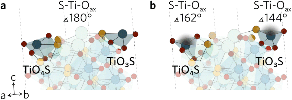 | ||
| Fig. 2 The (211) (a) unrelaxed and (b) relaxed surfaces highlighting the changes in S–Ti–Oax bond angles of the two different TiOxS. | ||
During the relaxation of slabs where Ti–Oax–Ti bonds were roughly parallel with the surface, the Oax in the surface layer was pushed up towards the vacuum. As can be seen in Fig. 3 for the (100) slab, the Ti–Oax–Ti bond angle typically decreased by about 15°. The effects of the relaxation on this bond tapered off quickly as the first subsurface Ti–Oax–Ti bond angle decreased by less than 5° in all slabs, while the second subsurface angle is closer to 180°.
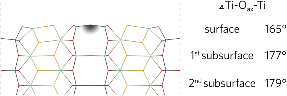 | ||
| Fig. 3 The (100) relaxed surface highlighting the layer-by-layer changes of the Ti–Oax–Ti bond angles parallel to the surface. | ||
The average bond distance was calculated for all four different bonds in the slabs using surfaxe. In all slabs, the bonds on the surface were significantly shorter compared to the bulk-like bond lengths. Select surface bond distance data can be found ESI Tables S1–S4,† while the bulk bond lengths can be seen in Table 1. The bond distances in the subsurface layer was typically slightly longer, which is in line with the expected pattern of relaxations normal to the surface. The surface unit layer is expected to contract when no reconstructions are observed to account for the extra energy from the dangling bonds on the surface, while the first subsurface layer expands to counteract that. A slight contraction is sometimes observed for the second subsurface layer, however the bulk-like bonding is regained in the third subsurface layer in all slabs. Where unit layers are composed of more than four atomic layers, the bulk-like behaviour is observed within the first subsurface layer.
The slab thicknesses at which the average bond distances converged to bulk-like can be found in Table 2. The convergence of slab thicknesses with respect to average bond lengths is limited by the convergence of bonds lengths in bonds that are most perpendicular to the surface. This is directly related to the aforementioned contraction and expansion of the unit layers due to excess energy on the surface. In all slabs the slowest convergence was seen for either the Ti–S or Y–S bonds, possibly because of longer bonding distances, indicating weaker bonding compared to M−O bonds. When TiO3S segments were exposed on the surface, S always displaced more than Oax, which had a bigger effect on the subsurface layers. The Ti–S bond lengths may seem unusually long in the bulk Y2Ti2O5S2 (2.87 Å) when compared to materials like TiS2 (2.43 Å) or TiS (2.47 Å), but they actually compare well with Ti–S bond lengths in La5Ti2AgS5O7 (2.90 Å) and La5Ti2CuS5O7 (2.80 Å) where a similar TiO5S octahedral environment is observed.38
| Miller index | Slab thickness (Å) | Unit layers | Atoms |
|---|---|---|---|
| (001) | 43 | 2 | 44 |
| (100) | 28 | 8 | 172 |
| (101) | 32 | 9 | 99 |
| (102) | 34 | 9 | 198 |
| (111) | 34 | 12 | 264 |
| (112) | 32 | 12 | 132 |
| (201) | 44 | 11 | 484 |
| (210) | 21 | 6 | 264 |
| (211) | 40 | 9 | 198 |
| (212) | 26 | 7 | 308 |
| (221) | 40 | 16 | 704 |
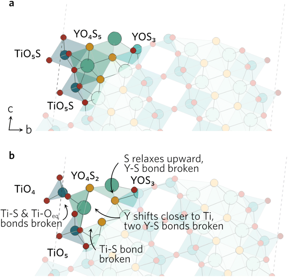
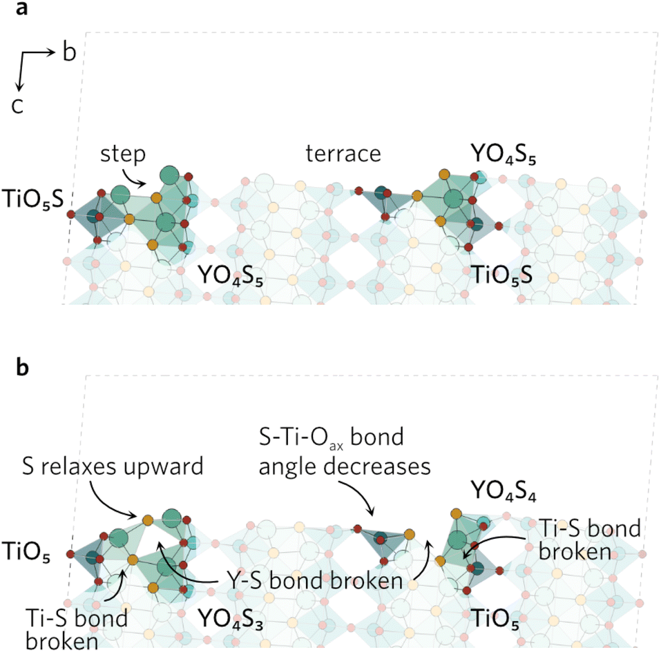
In a number of slabs the relaxations at the surface caused a slight change in coordination to some atoms in the surface and first subsurface layers. The contraction of the surface TiO3S into a tetrahedral-like shape in (111), (112), (210) and (221) resulted in the S atom displacing by over 1.5 Å. As the S atom displaced outwards, this led to an over 1 Å increase in the bond distance between S and Y in the subsurface layer, so that bond is effectively broken. The same process occurs on the (211) surface, however the description of the surface relaxation is complicated by the presence of a TiO4S unit on the surface. During the relaxation, the Ti–S bond distance in the TiO4S increases to 3.22 Å (shown with a dashed line in Fig. 2b), creating a TiO4 and keeping the subsurface layer coordination intact.
Perhaps the most striking differences in the surface and subsurface layers were seen in the (212) slab. The six cleaved Ti–O bonds led to many changes in coordination, driven by the relaxations of TiO3S and two Ti4OS. All three units relaxed identically to the counterparts on the (111), (112) and (211) surfaces. The last under-coordinated Ti on surface was left in a TiO3 unit with missing Ti–S and two Ti–Oeq bonds. During the relaxation the Oax–Ti–Oeq bond angle in the TiO3 increased from 104° to 119°, pushing the Oeq outwards. This relaxation breaks the Ti–Oeq bond in the subsurface layer.
In the (102) slab (see Fig. 4), the under-coordinated YOS3 on the surface flattened out during the relaxation to decrease the bond angle from 160° to 128°. This increases the Y–S bond length by 0.55 Å to 3.44 Å in the neighbouring fully-coordinated YO4S5, effectively breaking that bond. The increase also comes as a result of the Y atom of the YO4S5 unit relaxing towards the Ti, which breaks two Y–S bonds to S in the subsurface layer. Lastly, the largest displacement by any atom in the (102) slab was seen by the surface Ti in the TiO5S with Ti–S bond pointing outwards. The Ti atom shifts by over 0.8 Å towards the surface, breaking one of the Ti–Oeq bonds as bond distance increases to 2.67 Å. The Oax–Ti–Oeq angles in the newly formed TiO4 decrease to resemble an elongated tetrahedral shape.
 | ||
| Fig. 4 The (102) (a) unrelaxed and (b) relaxed surfaces. | ||
The clearly defined steps (see Fig. 5) on the (201) surface morph during the relaxation. The Oax–Ti–S bond angles of all four neighbouring ‘terrace’ TiO4S units decrease during the relaxation, which causes a discontinuity in the step. As the bond angles close up, the Y–S bond distance on the step increases to 3.84 Å, effectively rendering the bond broken. The change in the other step is governed by the relaxation of the under-coordinated YO3S2, where S relaxes upwards to flatten out to a square-pyramidal-like shape. The knock-on effects from this relaxation mean the bonding in the first subsurface layer of nearby atoms is disrupted, resulting in broken Ti–S and Y–S bonds.
 | ||
| Fig. 5 The (201) (a) unrelaxed and (b) relaxed surfaces. | ||
Slabs relaxed with hybrid HSE06 functional experienced the same relaxations as with PBEsol, so a repeat description is not necessary.
2.2 Surface energies and Wulff construction
Surface energies (γ) of relaxed slabs were calculated using the Fiorentini and Methfessel (FM) method, where the bulk energy (Ebulk,FM) is first derived from a line of best fit for a number of slab DFT energies (Eslab) for slabs with thickness M:| Eslab(M) = 2γ + MEbulk,FM. | (1) |
The surface energy is then calculated from the standard equation:
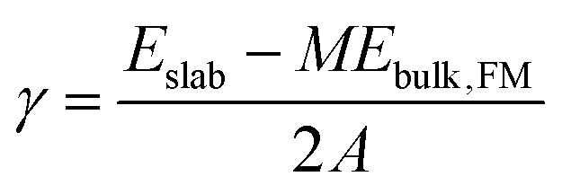 | (2) |
| Miller index | Cleavage energy | Surface energy |
|---|---|---|
| (001) | 0.41 | 0.39 |
| (100) | 1.48 | 1.03 |
| (101) | 1.43 | 0.99 |
| (102) | 2.83 | 1.99 |
| (111) | 2.91 | 1.73 |
| (112) | 2.77 | 1.61 |
| (201) | 1.73 | 1.14 |
| (210) | 2.09 | 1.17 |
| (211) | 2.05 | 1.15 |
| (212) | 2.36 | 1.35 |
| (221) | 2.93 | 1.75 |
Lower Miller index surfaces have lower cleavage and surface energies compared with higher order surfaces, likely a result of fewer bonds broken in the formation of the lower index surfaces. The (100) and (101) surfaces see modest 0.4 J m−2 reductions in energy upon relaxations, while the surface energy of (001) remains almost unchanged with a small 0.02 J m−2 difference in energy. The (101) surface is slightly lower in energy than (100) even though the opposite trend would be typically expected. This can be explained by considering the bonds broken during the cleavage as two Ti–Oeq and four Y–S bonds were broken on the (100) surface, while on the (101) only one Ti–Oeq, two Y–S and one Y–O bonds were broken. The 0.05 J m−2 difference in the cleavage energies between the two is maintained after the relaxation.
With the exception of the (201) surface, all higher order surfaces had cleavage energy exceed 2 J m−2. However, once they were relaxed, the surface energies were about 1 J m−2 lower than in energy, indicating a large relaxation had occurred. Referring back to the discussion earlier in Section 2.1, all the surfaces that saw a drastic reduction in excess energy were the ones where the surface TiO3S units were able to contract into a more tetrahedral shape.
Wulff construction of Y2Ti2O5S2 equilibrium form under thermodynamic limits was created based on the surface energies and the bulk lattice. The central idea behind the prediction of particle shape based on Wulff constructions is that lower energy surfaces will be more likely to form than higher energy surfaces. As shown in Fig. 6, this is indeed the case for Y2Ti2O5S2 Wulff shape. Unsurprisingly, the (001) facet occupies by far the largest area, covering over 55% of the total area. The other 45% is composed of the (101) facet covering 30% and the (211) facet covering 15% of the area. The (100) surface does not feature on the Wulff shape despite its energy being lower than that of the (211) surface.
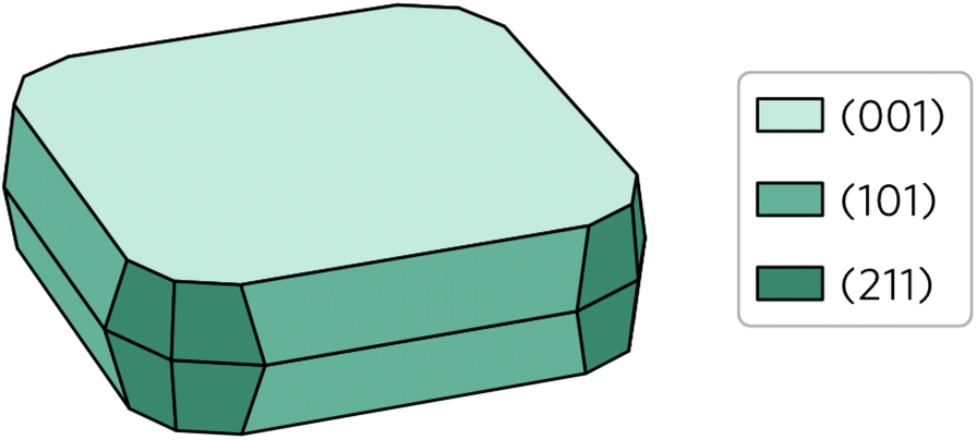 | ||
| Fig. 6 Wulff construction of Y2Ti2O5S2. The surfaces are colour coded so that the lighter shades represent lower surface energies and vice versa. | ||
The calculated Wulff construction is in excellent agreement with previously reported experimental particle shapes. Pan et al.39 described the synthesised particles as ‘plate-like’, with a clear basal (001) plane, which is in line with what we observe here. Considering they also report the particles like to form secondary clusters combining several primary particles, a visual comparison of the Wulff shape with the scanning electron microscopy images from the studies by Pan et al.39 and Wang et al.16 show good agreement between the two.
Nevertheless, the calculation of surface energies lacks the relation to the real-world conditions of photocatalytic water splitting, where the material would be submerged in water and exposed to air. While the surface eergy equation (eqn (2)) can be extended to include terms to account for solvation and adsorption of water molecules on the surface, the computational cost associated with the calculations of these terms outweighs their usefulness in this study. Still, some general trends and conclusions may be drawn from the literature. An increase in hydration generally leads to a decrease in surface energy, which means the higher energy surfaces would be more likely to experience a stabilising effect.40,41 The decrease in surface energies may also lead to a smaller range of surface energies, so the Wulff shape may become more isotropic.
2.3 Band alignment
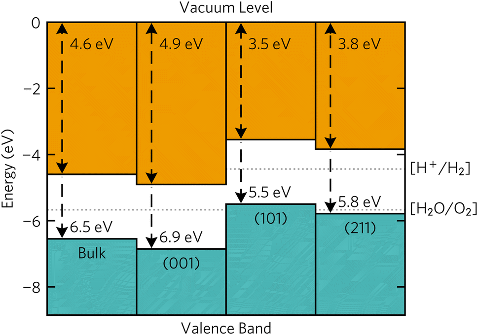
Band alignments of the Y2Ti2O5S2 surfaces that appeared on the Wulff shape were calculated using the core level alignment approach.42,43 The Oeq with two Ti and two Y atoms as nearest neighbours was chosen as the reference ‘core level’ atom to relate and compare the bulk and slab energies. Surfaxe was used to ensure the core level energy came from the Oeq closest to the mid-point of the slab. A more detailed description of calculation of the method used can be found in our previous work.18,38The surface band alignments are shown in Fig. 7 together with the bulk alignment. The (001) surface exhibits band alignment suitable for thermodynamic and kinetic photocatalysis of the oxygen half reaction with a large 1.1 eV overpotential at the valence band edge. Contrarily, the (101) and (211) surfaces are aligned for thermodynamic and kinetic photocatalysis of the hydrogen half reaction due to the 0.74 eV overpotential. The stark difference in band edge positions between surfaces can be ascribed to 1 eV larger surface dipole between the macroscopic planar potential and vacuum potential in the (001) surface (10.7 eV) compared to the (101) and (211) surfaces (9.5 eV). However, the macroscopic planar potential and core energies energy differences between the three surfaces are within 0.3 eV of each other, so the reason why the band edges are different must stem from the vacuum potential of the slabs.
 | ||
| Fig. 7 Calculated band alignments of bulk Y2Ti2O5S2 and the (001), (101) and (211) Y2Ti2O5S2 surfaces. Plotted with bapt.44 | ||
Similar variation in band offsets between different facts was observed in many other systems. The calculated ionisation potentials between different facets of SnS varied by as much as 0.9 eV from the lowest-energy (100) facet.45 In In2O3, a valence band offset of 0.7 eV was observed both experimentally from X-ray photoelectron spectroscopy (XPS) and computationally from hybrid-DFT for the non-polar (111) and polar (100) surfaces.46,47 The same computational study also showed a 0.5 eV offset between the non-polar (111) and (110) facets.47 The fluctuations were also seen in quinary La5Ti2MS5O7 (M = Ag, Cu) where the conduction bands of the (100), (101) and (1![[1 with combining macron]](https://www.rsc.org/images/entities/char_0031_0304.gif) 2) facets were offset from the other facets' conduction band edges by almost 2 eV.38
2) facets were offset from the other facets' conduction band edges by almost 2 eV.38
Combining the band edge positions with Wulff construction, it can be seen that the facets that favour each of the half-reactions are almost equally split. The spatial separation of the hydrogen and oxygen evolution facets has been observed experimentally. The efficiency of water splitting could be potentially improved if the deposition of reduction and oxidation co-catalysts was separated between the basal (001) facets and the side (101) and (211) facets.
Of course, as with the surface energies, the ionisation potentials and electron affinities are calculated under the assumption that the surfaces form an interface with vacuum. The presence of a surface/water interface in a real aqueous solution will alter the position of band edges, reflecting the intrinsic nature of the semiconductor.48 An upward shift of the bands due to the electron transfer between water and the material is expected for natively n-type semiconductors. Based on literature experimental results and the bulk band alignment favouring n-type behaviour based on doping rules, Y2Ti2O5S2 is expected to be intrinsically n-type, so an upward shift of band edges may be expected. This is in line with experimental observations of photocatalytic activity, as poorer O2 evolution rates are expected based on the lower kinetic overpotential available on the (001) surface.
Accurately quantifying the band offsets from solvation of water on Y2Ti2O5S2 is beyond the scope of this study as it would be prohibitively expensive to do at a hybrid-DFT level. Nevertheless, the literature offers some suggestions on the quantitative effects of the solvation. Stevanović et al.49 showed that when pH equals the point of zero charge, the effect of the aqueous solution can be approximated by a 0.5 eV upward shift of band edges for metal oxides.
2.4 Identifying surface active sites
It is widely recognised that surface photocatalytic activity can be enhanced by modifying its surfaces using defect engineering. For example, in In2O3 a 15-fold improvement in visible light photocurrent was noted when the oxygen vacancies were introduced on the surface of the porous sheets.50 Similarly, about 3% (atom) concentration of oxygen vacancies in SrTiO3 improved the hydrogen evolution rates under UV-visible light by 2.3-fold compared to the unmodified SrTiO3.51A full intrinsic point defects study for the Y2Ti2O5S2 surfaces is well beyond the scope of this study, however Madelung potential can be used in lieu as a coarse prediction tool for defect behaviour. Madelung potential indicates the cohesive strength around a site in the lattice of an ionic solid. Its magnitude is determined by the charge and distance of the site's nearest neighbours, so changes in coordination environment around the different surface sites would result in varying Madelung potentials. Generally, the lower the Madelung potential on an anion site, the more likely a vacancy is to form there, and the less negative the Madelung potential is on a cation site, the more likely electrons are to accumulate on it.
Here, we only consider the surfaces that appear on the Wulff shape, i.e. the (001), (101) and (211) facets, but similar behaviour can be expected on other surfaces as well. Madelung potentials for the bulk Y2Ti2O5S2 and the three surfaces were calculated using the Ewald summation method implemented in pymatgen and can be found in ESI Tables S1–S4.† To determine coordination environments, a maximum bond distance of 3 Å was used for Y, Ti and S and a lower threshold of 2.5 Å was used for O to avoid the spurious assignation of O–O bonding. Madelung potentials for Y were calculated for completeness but as Y states do not constitute the electronic band edges, Y sites are unlikely to be electronically active.
The Madelung potentials of Ti on the (001) and (101) surfaces are all within 0.5 V of the bulk-like potential. Because of the nature of the (211) surface cleavage, more changes to the coordination were seen; however, only two surface Ti see large changes to their electrostatic potential. The calculated potential of the under-coordinated Ti in the TiO3S motif in Fig. 8 is 3.2 V less negative than bulk-like; while the Madelung potential of the only fully-coordinated Ti on the surface is 4.2 V more negative.
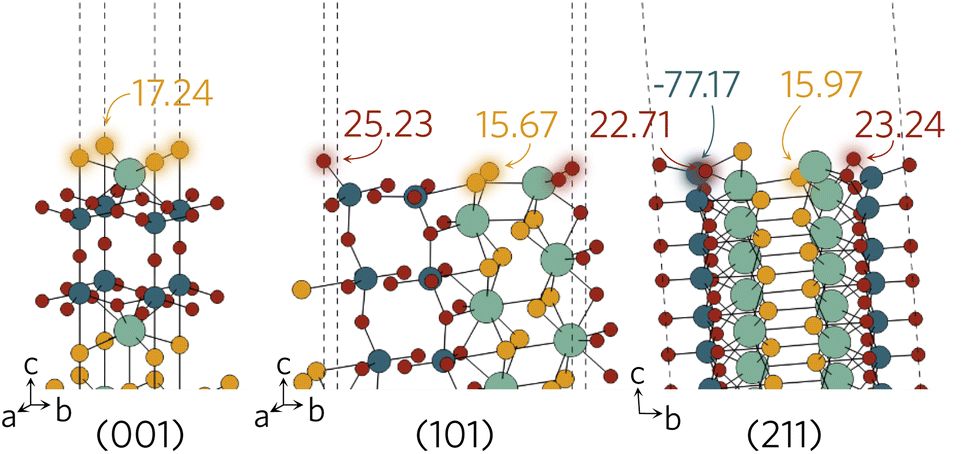 | ||
| Fig. 8 Surface active sites on (001), (101) and (211) surfaces shown with an aural glow with the corresponding Madelung potential of each site in V. | ||
Of the two distinct oxygen sites, Oax is expected to be less likely to form a vacancy due to demonstrating at least 1 V higher potential compared to the Oeq. There are no oxygens directly on the surface of the (001) slab and Madelung potentials reveal all have bulk-like values. This is of course not unexpected as the structure remains largely bulk-like after the geometry optimisation. A larger difference is seen on the (101) and (211) surfaces where the majority of under-coordinated surface oxygens experience a lower Madelung potential than those in the bulk-like region. Between the different surface sites, the greatest variation in potential was seen on the (211) surface, where the two-coordinate Oeq experience up to 6 V lower potential than the fully-coordinate counterparts (highlighted in Fig. 8). The opposite was found when analysing the sulphur Madelung potentials where the two-coordinate S in the TiO3S highlighted in Fig. 2b experiences the second highest surface Madelung potential due to the short Ti–S bond (2.32 Å).
The possible active sites based on Madelung potential analysis on the (001), (101) and (211) surfaces are summarised in Fig. 8. Clearly, the under-coordinated S and Oeq atoms with longer-than-average bond distances to neighbouring Y and Ti will form vacancies more readily than other surface anions. As the conduction band minimum is comprised of Ti d states, it follows that, when ionised, the charge is likely to accumulate on the under-coordinated Ti, reducing it to Ti3+. Obviously, we only considered what would happen to anion vacancies and where charge would accumulate on the cations. Intrinsic interstitials and antisites, as well as extrinsic dopants will also affect the photocatalytic activity and likely introduce other surface active sites, so further work is necessary to fully describe the Y2Ti2O5S2 surface defect chemistry.
2.5 Bulk optoelectronic properties
The optical absorption spectrum calculated with the HSE06 functional in Fig. 9a shows a slow onset of absorption at 1.95 eV from the fundamental band gap, while the Tauc plot in Fig. 9b reveals a optical band gap of 2.28 eV. The irreducible representations analysis reveals the optical transition from the doubly-degenerate valence band maximum (VBM) to conduction band minimum (CBM) is parity allowed but is expected to be weak. From the topmost valence band, the band gap is 1.95 eV all the way along the Γ–Z direction where the band edges are perfectly flat. In theory an optical transition could occur, but Z–Z transitions are parity forbidden. Transitions at both N and X are parity allowed, but as the curvature in both valence and conduction bands is greater in Γ–N and Γ–X directions, the band gap rapidly increases until other combinations of transitions around band edges are lower in energy. The VBM to CBM+1 (0.30 eV above CBM) transition is symmetry forbidden; however, VBM−1 (0.32 eV below the VBM) to CBM is allowed. The latter VBM−1 to CBM transition is stronger and with an energy gap of 2.26 eV lines up well with the Tauc band gap.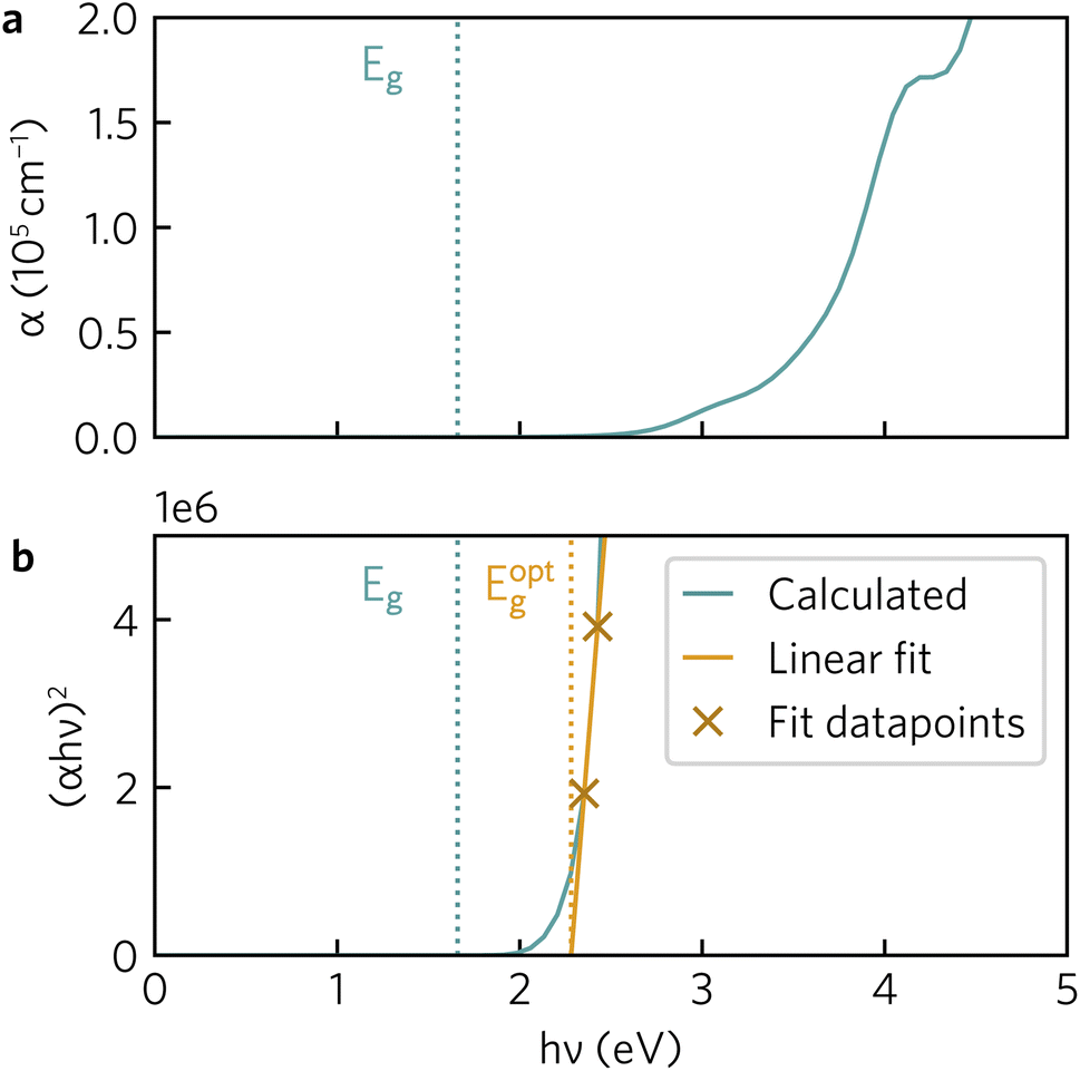 | ||
| Fig. 9 (a) Y2Ti2O5S2 HSE06-calculated absorption coefficients (α). (b) Tauc plot with line of best fit. Both plots include Gaussian smearing of 0.15 to improve readability. Fundamental (Eg, 1.95 eV) and optical (Eoptg, 2.28 eV) band gaps indicated in a dotted line. | ||
To further aid in the characterisation of Y2Ti2O5S2 as a photocatalyst, we explored its excitonic properties theoretically using many-body perturbation theory. First, we calculated the quasiparticle band structure using the QSGW and QSGŴ methods, to compare with our hybrid DFT calculations, using the HSE06 relaxed geometry. The band structures calculated with QSGŴ is depicted in Fig. 10, while the QSGW electronic structure can be found in the ESI Fig. S1.†
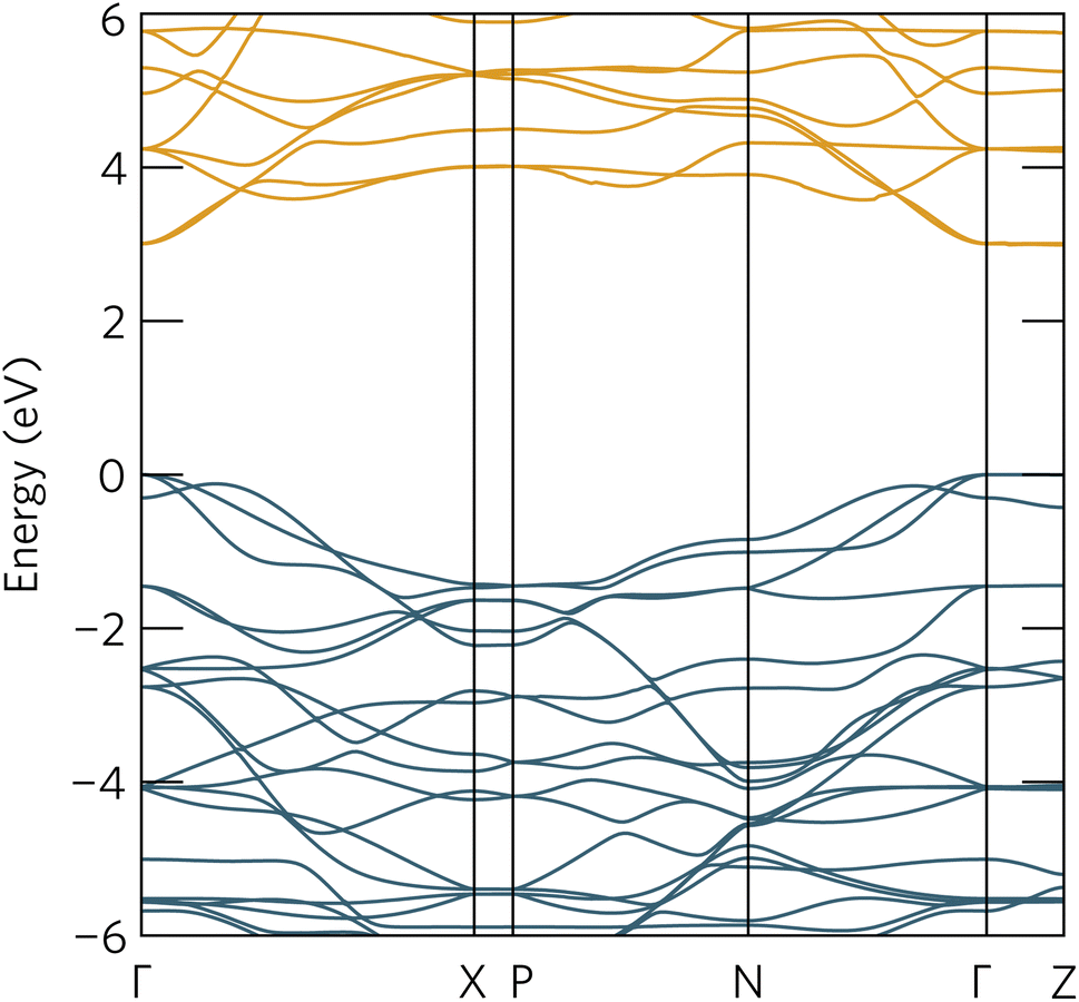 | ||
| Fig. 10 The quasiparticle band structure of Y2Ti2O5S2, calculated within QSGŴ method. The chosen k-path across the Brillouin Zone uses notation from Bradley and Cracknell.52 Valence bands are depicted in blue, conduction bands in orange, the valence band maximum is set to 0 eV, and the figure has been plotted using the sumo package.53 | ||
Initially, it is evident that the core features of the band structure, such as the dispersion along Γ to X and the correspondent localisation of states along Γ to Z are replicated in both quasiparticle methods here, as well as the HSE06 band structure. A minor change from HSE06 is the increased splitting of the degenerate Ti d conduction bands along Γ to N. More significantly, the quasiparticle gap is significantly greater −3.05 eV with QSGW compared to the fundamental HSE06 gap of 1.95 eV. QSGW is expected to systematically overestimate band gaps due to the omission of the vertex and incomplete screening effects within the RPA, typically only by 10% in s/p semiconductors, but the effect can be much larger in Mott–Hubbard insulators such as NiO.32 The addition of ladder diagrams, and thus additional screening due to the electron–hole interactions, to the screened Coulomb W in the QSGŴ method is expected to account for the majority of the latter effect – in Y2Ti2O5S2, it does reduce the gap, but only by 60 meV to 2.99 eV. This difference in band gap, of over 1 eV between the hybrid DFT and quasiparticle band structures, is considerable, though is similar to that seen in the caesium titanium halides, which similarly have an anionic-dominated valence band and Ti d conduction band.54,55 This difference will be revisited when considering the optical spectrum.
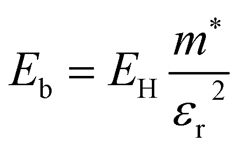 | (3) |
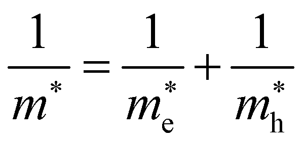 . The electronic structure of Y2Ti2O5S2 is highly anisotropic between the in-plane (xy) and out-of-plane (z) directions, so the simple hydrogenic model is not the most suitable. To account for the anisotropy, the eqn (3) is modified to describe a two-dimensional (2D) system:
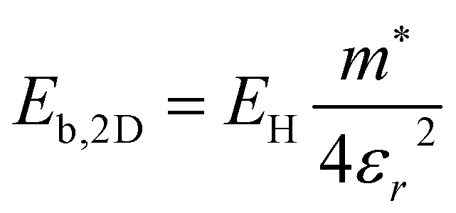 | (4) |
 | (5) |
Using the electron and hole effective masses 0.82 me and 0.44 me, respectively, and the calculated static dielectric constant of 30, the predicted exciton binding energy of Y2Ti2O5S2 is 1 meV. For photocatalysts for water splitting, the binding energy should be less than thermal energy (kBT), which is around 25 meV at room temperature. Evidently this crude estimate shows efficient separation of the charge carriers is possible at low temperatures.
To fully understand the excitonic properties of Y2Ti2O5S2, however, we can explicitly calculate the electron–hole pair through the solution of the BSE. In single-shot methods such as G0Ŵ0 + BSE, all excitonic effects are combined and so by using QSGŴ for the underlying self-energy, any quasiparticle gap renormalisation as a result of electron–hole screening has already been accounted for. Thus, by comparing QSGŴ + RPA and QSGŴ + BSE spectra the exciton binding energy can be directly extracted. In Fig. 11, the imaginary dielectric spectrum calculated with QSGŴ + RPA and QSGŴ + BSE are depicted and the resultant absorption coefficients compared with HSE06.
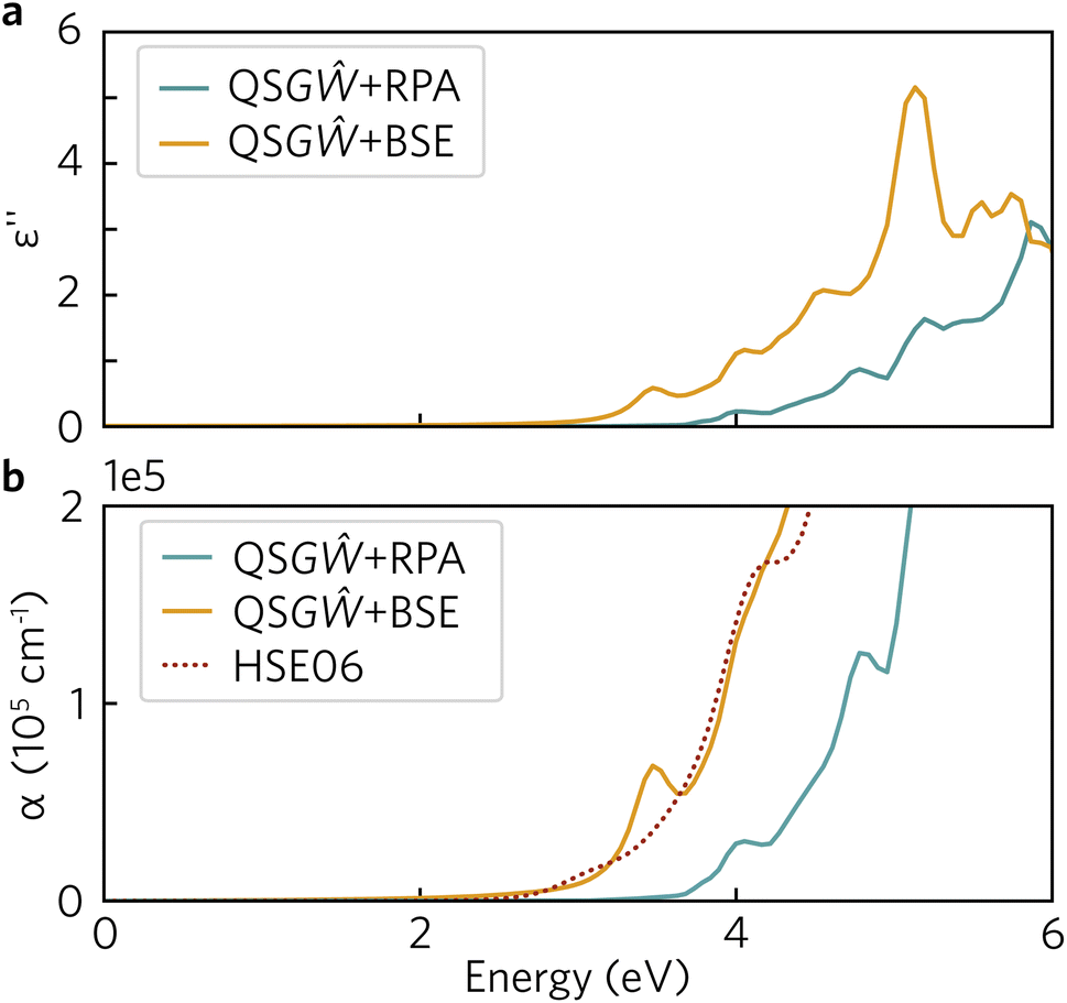 | ||
| Fig. 11 (a) Imaginary dielectric spectrum, calculated with QSGŴ + RPA and QSGŴ + BSE with an inherent smearing of 0.01 Ry; (b) Absorption coefficient, calculated with QSGŴ + RPA and QSGŴ + BSE and HSE06 – an additional Gaussian smearing of 0.02 eV was added to the QSGŴ spectra to match that of the HSE06 spectrum. | ||
In Fig. 11a, a large excitonic effect is clear, with a red-shift of the onset of the BSE spectrum of at least 0.5 eV. The major band-to-band peaks in the RPA are also replicated, with the transition at 5 eV being further augmented in intensity. While there is no strong excitonic peak below the 2.99 eV quasiparticle gap, the absorption is non-zero as a result of a series of weakly allowed excitonic transitions: 2.59, 2.72, 2.87, 2.91 and 2.94 eV. Each of these transitions is two-fold degenerate, with one component being forbidden (dark) and the other being very weakly allowed along x/y – this behaviour would partly align with the above finding in the HSE06 optical calculations that the fundamental gap at Γ is weakly allowed, and is parity forbidden across the flat bands between Γ and Z. The theoretical exciton binding energy is thus 0.4 eV, significantly higher than that predicted from the Wannier–Mott model – even when including the possibility of a 2D exciton due to the anisotropic electronic structure. It may be noted that although Y2Ti2O5S2 is predicted to have a high static dielectric constant, the high frequency component (seen in ESI Fig. S2†) is relatively small (∼4.6). Using the high-frequency dielectric constant alone, the 2D Wannier–Mott model would predict an order of magnitude increase in the exciton binding energy to 28 meV, though this would still be an order of magnitude lower than that predicted by the BSE calculations.
Further explanation may be provided by analysing the contributions to the sub-gap excitonic transitions, as shown by a projection of the contributions to the 2.59 eV excitonic wavefunction back onto the quasiparticle band structure, as shown in Fig. 12. The exciton demonstrates a hybrid behaviour between Wannier–Mott and Frenkel behaviour. As expected, contribution from the valence and conduction band arises from all k-points across Γ and Z, consistent with complete localisation in that direction and thus a 2D exciton; along the other directions from Γ, there are however still significant contributions from multiple k-points, despite the low effective masses of both electrons and holes in that direction. Most notably, in the valence band, there is additional contribution from the band below (‘VB−1’) where it crosses the highest energy band, particularly along Γ to X: this mixing may explain why the exciton transitions are further partially allowed as detailed above.
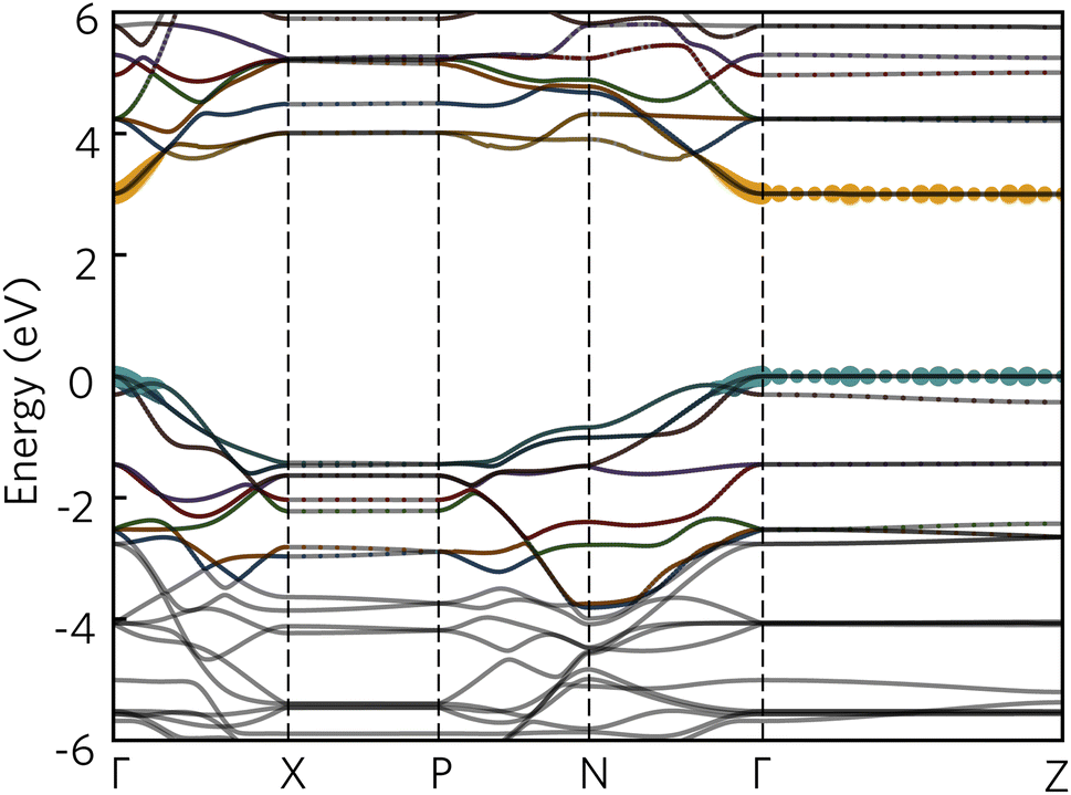 | ||
| Fig. 12 The quasiparticle band structure of Y2Ti2O5S2, calculated within QSGŴ method, with the magnitudes of individual state contributions to the first bright exciton (2.59 eV) projected onto the band structure. The chosen path across the Brillouin Zone uses notation from Bradley and Cracknell.52 Excitonic contributions from the valence bands are depicted in blue and conduction bands in orange, and was plotted with software included within the Questaal package.30 | ||
It is also possible to draw comparison to recent findings with G0Ŵ0 + BSE on anatase TiO2, which despite low effective masses, high dielectric behaviour and a 3D-connected crystal structure has recently predicted to have a strongly bound Frenkel-type exciton with 2D character.56 Baldini et al.56 rationalise the existence of such a localised exciton (with many states contributing to the transition) through the parallel curvature of valence and conduction bands in the electronic structure of anatase meaning electron and hole states have similar group velocities across a section of the Brillouin Zone. In Y2Ti2O5S2 not only are the valence and conduction bands parallel across Γ to Z, but ‘VB−1’ and the CBM are also parallel along Γ to X and along Γ to N, potentially leading to further localisation in other Cartesian directions as well, and a high exciton binding energy.
Nevertheless, with a binding energy of 0.4 eV, there is still a discrepancy between the predicted optical spectrum here and experimental photoluminescence emission that is observed centred around 2.0 eV.57 The QSGŴ method still does not include multiple effects that could further change the predicted optical behaviour of Y2Ti2O5S2, such as coupling of electrons or excitons to the lattice, or more complex phenomena such as bi-excitons or association of excitons with a defect centre. The former could be responsible for the larger portion of the observed discrepancy against experiment: a full study of exciton-phonon coupling is beyond the scope of this study, however, the approximate magnitude of the effect may be considered. The zero-point renormalisation of the gap of rutile TiO2 was recently calculated with ab initio methods to be 0.35 eV;58 were Y2Ti2O5S2 to demonstrate a reduction in quasiparticle gap by a similar magnitude, this would lead to the QSGŴ + BSE optical onset lying close to that observed experimentally. It is clear that further detailed study of the excitons in Y2Ti2O5S2 using both theoretical and experimental methods is necessary to properly characterise its optical properties and fully understand its capability as a photocatalyst.
A remaining question is then the suitability of hybrid DFT as a predictive tool, given that Y2Ti2O5S2 is predicted to be highly excitonic within many-body perturbation theory. In Fig. 11b, the absorption coefficients calculated using the three theoretical methods are compared within the relevant spectral region (up to the near-mid UV), and it is evident, that despite the absence of many-body effects within DFT, the HSE06 optical absorption matches very well to that of QSGŴ + BSE in both the slow initial onset followed and the strengthening above 3 eV, with the exception of the excitonically-enhanced peak in the latter above the quasiparticle gap. While this agreement may be fortuitous – though it may be noted that the functional form of HSE06 includes the effect of screening on the exchange interaction – it demonstrates that HSE06 can be reliable at generally predicting the optical behaviour and onset of Y2Ti2O5S2, and thus that the trends established using hybrid DFT are valid in comparison with higher-level theoretical methods.
3 Conclusions
In this work, we investigated the structures, energetics and electronic band alignments of clean Y2Ti2O5S2 non-polar surfaces with a maximum Miller index of 2 using DFT calculations, utilising both generalised gradient approximation and hybrid functionals. We outline the main relaxation patterns of the surfaces, which primarily occur when the TiO5S octahedra are cleaved along the Oax–Ti–S bond when surfaces are created.Cleavage energies of the eleven studied Miller indices, calculated using the Fiorentini–Methfessel approach, all fall in the relatively wide 0.41–2.93 J m−2 range. The relaxed surface energies were up to 1 J m−2 lower compared to the cleavage energies, covering a slightly narrower 0.39–1.99 J m−2 range. The (001) surface was found to be the most stable with a surface energy of 0.39 J m−2. Only three surfaces, (001), (101) and (211), appeared on the Wulff construction representing the equilibrium form of Y2Ti2O5S2 at the thermodynamic limit. Overall, the general plate-like shape with the basal (001) plane agrees well with the reported experimental particle morphology.
The band alignment of the clean surfaces that appear on the Wulff shape agrees well with the experimentally observed spatial separation of hydrogen and oxygen evolution facets. The band alignment of the basal (001) surface suggests good overpotential for the oxygen evolution reaction, while the side (101) and (211) surfaces exhibit sufficient overpotential for hydrogen evolution. As this study was done assuming the surfaces are in vacuum, rather than in a aqueous medium, more future work would be needed to confirm the alignment in solution.
Potential surface active sites on the (001), (101) and (211) surfaces were identified using site Madelung potentials. Generally, sulphur and equatorial oxygen vacancies are expected to be the dominant surface active sites. On the (001) surface only the sulphur atoms experienced any variation in electrostatic potential, while both under-coordinated sulphur and equatorial oxygen sites are potential active site candidates on the (101). Due to the more complex cleavage direction on the (211) surface, larger differences in Madelung potentials between surface and bulk-like sites were observed. In addition to the sulphur and equatorial oxygen sites, the under-coordinated Ti could act as an active site, facilitating water redox by getting reduced to Ti3+.
The optical absorption of Y2Ti2O5S2, as calculated with both hybrid DFT and QSGŴ + BSE methods demonstrates a slow onset due to forbidden transitions at the fundamental gap, with stronger absorption at energies above 3 eV. Furthermore, QSGŴ + BSE calculations that explicitly include electron–hole interaction, predict an exciton binding energy of 0.4 eV, indicating at least partial Frenkel behaviour. A tightly bound 2D exciton is predicted as a result of not only the localisation of electrons and holes in the crystallographic z direction, but also additional mixing of multiple valence bands into the excitonic wavefunction. These results indicate that to fully understand the promise of Y2Ti2O5S2 as a photocatalyst, its optical and excitonic behaviour needs further consideration.
Author contributions
KB: investigation, methodology, data curation, formal analysis, visualisation, writing – original draft. CNS: investigation, formal analysis, writing – original draft. DOS: funding acquisition, supervision, writing – review & editing.Conflicts of interest
There are no conflicts to declare.Acknowledgements
KB and DOS acknowledge support from the European Research Council, ERC (grant no. 758345). CNS is grateful to the Ramsay Memorial Fellowship Trust and the Department of Chemistry at UCL for the funding of a Ramsay Fellowship. We are grateful to the UK Materials and Molecular Modelling Hub for computational resources, which is partially funded by EPSRC (EP/P020194/1 and EP/T022213/1) and to UCL for the provision of the Kathleen (Kathleen@UCL) supercomputer. DOS acknowledges support from the EPSRC(EP/N01572X/1). DOS acknowledges membership of the Materials Design Network. Via our membership of the UK HEC Materials Chemistry Consortium, which is funded by the UK Engineering and Physical Sciences Research Council (EP/R029431), this work used the ARCHER2 UK National Supercomputing Service (http://www.archer2.ac.uk).Notes and references
- N. Rambhujun, M. S. Salman, T. Wang, C. Pratthana, P. Sapkota, M. Costalin, Q. Lai and K.-F. Aguey-Zinsou, MRS Energy Sustain., 2020, 7, 33 CrossRef.
- S. Z. Baykara, Int. J. Hydrogen Energy, 2018, 43, 10605–10614 CrossRef CAS.
- M. Ji and J. Wang, Int. J. Hydrogen Energy, 2021, 46, 38612–38635 CrossRef CAS.
- R. W. Howarth and M. Z. Jacobson, Energy Sci. Eng., 2021, 9, 1676–1687 CrossRef CAS.
- R. W. Howarth and M. Z. Jacobson, Energy Sci. Eng., 2022, 10, 1955–1960 CrossRef.
- A. Fujishima and K. Honda, Nature, 1972, 238, 37–38 CrossRef CAS PubMed.
- T. Kawai and T. Sakata, J. Chem. Soc., Chem. Commun., 1980, 694 RSC.
- A. L. Linsebigler, G. Lu and J. T. Yates, Chem. Rev., 1995, 95, 735–758 CrossRef CAS.
- A. A. Nada, M. H. Barakat, H. A. Hamed, N. R. Mohamed and T. N. Veziroglu, Int. J. Hydrogen Energy, 2005, 30, 687–691 CrossRef CAS.
- D. O. Scanlon, C. W. Dunnill, J. Buckeridge, S. A. Shevlin, A. J. Logsdail, S. M. Woodley, C. R. A. Catlow, M. J. Powell, R. G. Palgrave, I. P. Parkin, G. W. Watson, T. W. Keal, P. Sherwood, A. Walsh and A. A. Sokol, Nat. Mater., 2013, 12, 798–801 CrossRef CAS.
- T. Le Bahers, M. Rérat and P. Sautet, J. Phys. Chem. C, 2014, 118, 5997–6008 CrossRef.
- G. Zhang, Z. Guan, J. Yang, Q. Li, Y. Zhou and Z. Zou, Sol. RRL, 2022, 202200587 Search PubMed.
- C. Boyer-Candalen, J. Derouet, P. Porcher, Y. Moëlo and A. Meerschaut, J. Solid State Chem., 2002, 165, 228–237 CrossRef CAS.
- M. Goga, R. Seshadri, V. Ksenofontov, P. Gütlich and W. Tremel, Chem. Commun., 1999, 979–980 RSC.
- A. Ishikawa, T. Takata, T. Matsumura, J. N. Kondo, M. Hara, H. Kobayashi and K. Domen, J. Phys. Chem. B, 2004, 108, 2637–2642 CrossRef CAS.
- Q. Wang, M. Nakabayashi, T. Hisatomi, S. Sun, S. Akiyama, Z. Wang, Z. Pan, X. Xiao, T. Watanabe, T. Yamada, N. Shibata, T. Takata and K. Domen, Nat. Mater., 2019, 18, 827–832 CrossRef CAS.
- L. Lin, V. Polliotto, J. J. M. Vequizo, X. Tao, X. Liang, Y. Ma, T. Hisatomi, T. Takata and K. Domen, ChemPhotoChem, 2022, 6, e202200209 CrossRef CAS.
- K. Brlec, K. B. Spooner, J. M. Skelton and D. O. Scanlon, J. Mater. Chem. A, 2022, 10, 16813–16824 RSC.
- K. McColl and F. Corà, J. Mater. Chem. A, 2021, 9, 7068–7084 RSC.
- P. E. Blöchl, Phys. Rev. B: Condens. Matter Mater. Phys., 1994, 50, 17953–17979 CrossRef.
- G. Kresse and J. Furthmüller, Comput. Mater. Sci., 1996, 6, 15–50 CrossRef CAS.
- G. Kresse and J. Furthmüller, Phys. Rev. B: Condens. Matter Mater. Phys., 1996, 54, 11169–11186 CrossRef CAS.
- G. Kresse and D. Joubert, Phys. Rev. B: Condens. Matter Mater. Phys., 1999, 59, 1758–1775 CrossRef CAS.
- J. P. Perdew, A. Ruzsinszky, G. I. Csonka, O. A. Vydrov, G. E. Scuseria, L. A. Constantin, X. Zhou and K. Burke, Phys. Rev. Lett., 2008, 100, 136406 CrossRef.
- J. Heyd, G. E. Scuseria and M. Ernzerhof, J. Chem. Phys., 2003, 118, 8207–8215 CrossRef CAS.
- A. V. Krukau, O. A. Vydrov, A. F. Izmaylov and G. E. Scuseria, J. Chem. Phys., 2006, 125, 224106 CrossRef.
- P. Pulay, Mol. Phys., 1969, 17, 197 CrossRef CAS.
- K. Momma and F. Izumi, J. Appl. Crystallogr., 2011, 44, 1272–1276 CrossRef CAS.
- K. Brlec, D. W. Davies and D. O. Scanlon, J. Open Source Softw., 2021, 6, 3171 CrossRef.
- D. Pashov, S. Acharya, W. R. L. Lambrecht, J. Jackson, K. D. Belashchenko, A. Chantis, F. Jamet and M. van Schilfgaarde, Comput. Phys. Commun., 2020, 249, 107065 CrossRef CAS.
- T. Kotani, M. van Schilfgaarde and S. V. Faleev, Phys. Rev. B: Condens. Matter Mater. Phys., 2007, 76, 165106 CrossRef.
- B. Cunningham, M. Grüning, D. Pashov and M. van Schilfgaarde, QSGŴ: Quasiparticle Self Consistent GW with Ladder Diagrams in W, 2023, http://arxiv.org/abs/2302.06325 Search PubMed.
- B. Cunningham, M. Grüning, P. Azarhoosh, D. Pashov and M. van Schilfgaarde, Phys. Rev. Mater., 2018, 2, 034603 CrossRef CAS.
- J. Buckeridge and D. O. Scanlon, Phys. Rev. Mater., 2019, 3, 051601 CrossRef CAS.
- P. A. E. Murgatroyd, M. J. Smiles, C. N. Savory, T. P. Shalvey, J. E. N. Swallow, N. Fleck, C. M. Robertson, F. Jäckel, J. Alaria, J. D. Major, D. O. Scanlon and T. D. Veal, Chem. Mater., 2020, 32, 3245–3253 CrossRef CAS PubMed.
- G. Hyett, O. J. Rutt, Z. A. Gál, S. G. Denis, M. A. Hayward and S. J. Clarke, J. Am. Chem. Soc., 2004, 126, 1980–1991 CrossRef CAS.
- Materials Data on Y2Ti2S2O5 (SG:139) by Materials Project, 2016 Search PubMed.
- K. Brlec, S. R. Kavanagh, C. N. Savory and D. O. Scanlon, ACS Appl. Energy Mater., 2022, 5, 1992–2001 CrossRef CAS PubMed.
- Z. Pan, H. Yoshida, L. Lin, Q. Xiao, M. Nakabayashi, N. Shibata, T. Takata, T. Hisatomi and K. Domen, Res. Chem. Intermed., 2021, 47, 225–234 CrossRef CAS.
- S. G. Srinivasan, R. Shivaramaiah, P. R. C. Kent, A. G. Stack, A. Navrotsky, R. Riman, A. Anderko and V. S. Bryantsev, J. Phys. Chem. C, 2016, 120, 16767–16781 CrossRef CAS.
- F. Zasada, W. Piskorz, S. Cristol, J.-F. Paul, A. Kotarba and Z. Sojka, J. Phys. Chem. C, 2010, 114, 22245–22253 CrossRef CAS.
- Y. Hinuma, F. Oba, Y. Kumagai and I. Tanaka, Phys. Rev. B: Condens. Matter Mater. Phys., 2012, 86, 245433 CrossRef.
- Y. Hinuma, A. Grüneis, G. Kresse and F. Oba, Phys. Rev. B: Condens. Matter Mater. Phys., 2014, 90, 155405 CrossRef.
- A. Ganose, Band Alignment Plotting Tool (Bapt), 2022 Search PubMed.
- V. Stevanović, K. Hartman, R. Jaramillo, S. Ramanathan, T. Buonassisi and P. Graf, Appl. Phys. Lett., 2014, 104, 211603 CrossRef.
- M. V. Hohmann, P. Ágoston, A. Wachau, T. J. M. Bayer, J. Brötz, K. Albe and A. Klein, J. Phys.: Condens. Matter, 2011, 23, 334203 CrossRef.
- A. Walsh and C. R. A. Catlow, J. Mater. Chem., 2010, 20, 10438 RSC.
- K.-W. Park and A. M. Kolpak, Commun. Chem., 2019, 2, 79 CrossRef.
- V. Stevanović, S. Lany, D. S. Ginley, W. Tumas and A. Zunger, Phys. Chem. Chem. Phys., 2014, 16, 3706 RSC.
- F. Lei, Y. Sun, K. Liu, S. Gao, L. Liang, B. Pan and Y. Xie, J. Am. Chem. Soc., 2014, 136, 6826–6829 CrossRef CAS PubMed.
- H. Tan, Z. Zhao, W.-b. Zhu, E. N. Coker, B. Li, M. Zheng, W. Yu, H. Fan and Z. Sun, ACS Appl. Mater. Interfaces, 2014, 6, 19184–19190 CrossRef CAS PubMed.
- C. J. Bradley and A. P. Cracknell, The Mathematical Theory of Symmetry in Solids: Representation Theory for Point Groups and Space Groups, Clarendon Press, Oxford, 1972 Search PubMed.
- A. M. Ganose, A. J. Jackson and D. O. Scanlon, J. Open Source Softw., 2018, 3, 717 CrossRef.
- S. R. Kavanagh, C. N. Savory, S. M. Liga, G. Konstantatos, A. Walsh and D. O. Scanlon, J. Phys. Chem. Lett., 2022, 13, 10965–10975 CrossRef CAS PubMed.
- B. Cucco, G. Bouder, L. Pedesseau, C. Katan, J. Even, M. Kepenekian and G. Volonakis, Appl. Phys. Lett., 2021, 119, 181903 CrossRef CAS.
- E. Baldini, L. Chiodo, A. Dominguez, M. Palummo, S. Moser, M. Yazdi-Rizi, G. Auböck, B. P. P. Mallett, H. Berger, A. Magrez, C. Bernhard, M. Grioni, A. Rubio and M. Chergui, Nat. Commun., 2017, 8, 13 CrossRef CAS.
- R. Li, Z. Zha, Y. Zhang, M. Yang, L. Lin, Q. Wang, T. Hisatomi, M. Nakabayashi, N. Shibata, K. Domen and Y. Li, J. Mater. Chem. A, 2022, 10, 24247–24257 RSC.
- M. Engel, H. Miranda, L. Chaput, A. Togo, C. Verdi, M. Marsman and G. Kresse, Phys. Rev. B, 2022, 106, 094316 CrossRef CAS.
Footnote |
| † Electronic supplementary information (ESI) available: Input and output files from surface calculations, including scripts used in slab generation, analysis and post-processing, as well as GW input files are available from Zenodo. The supplied PDF contains the QSGW band structure, plot of convergence of optical properties with respect to k-mesh, bulk and surface Madelung potentials and a link to Zenodo repository. See DOI: https://doi.org/10.1039/d3ta02801a |
| This journal is © The Royal Society of Chemistry 2023 |