DOI:
10.1039/D3SC04317G
(Edge Article)
Chem. Sci., 2023,
14, 12661-12675
Hybrid classical/machine-learning force fields for the accurate description of molecular condensed-phase systems†
Received
17th August 2023
, Accepted 24th October 2023
First published on 31st October 2023
Abstract
Electronic structure methods offer in principle accurate predictions of molecular properties, however, their applicability is limited by computational costs. Empirical methods are cheaper, but come with inherent approximations and are dependent on the quality and quantity of training data. The rise of machine learning (ML) force fields (FFs) exacerbates limitations related to training data even further, especially for condensed-phase systems for which the generation of large and high-quality training datasets is difficult. Here, we propose a hybrid ML/classical FF model that is parametrized exclusively on high-quality ab initio data of dimers and monomers in vacuum but is transferable to condensed-phase systems. The proposed hybrid model combines our previous ML-parametrized classical model with ML corrections for situations where classical approximations break down, thus combining the robustness and efficiency of classical FFs with the flexibility of ML. Extensive validation on benchmarking datasets and experimental condensed-phase data, including organic liquids and small-molecule crystal structures, showcases how the proposed approach may promote FF development and unlock the full potential of classical FFs.
1. Introduction
An accurate description of the physical interactions between atoms in condensed-phase molecular systems remains one of the biggest challenge in computational chemistry. Electronic structure methods are in principle able to describe properties of such systems reliably.1,2 However, access to long time-scales and large systems is severely limited by the associated computational cost. Due to the computational complexity of electronic structure methods, this issue is unlikely to be resolved solely by additional computational power in the near future.3 As a solution, approximate methods, such as force fields (FFs)4 or semi-empirical quantum chemistry methods, have been developed.5,6 Especially FFs enable routine access to large systems at microsecond time scales.7 However, approximations inherent to FFs and semi-empirical methods limit their ability to describe certain interactions, for instance polarization.8,9
With the development of machine learning (ML) potentials during the last decade (see e.g. refs. 10–13), a new paradigm has emerged for the computational study of atomic systems. Thanks to the fast-paced development of underlying architectures, ML potentials achieve now routinely errors on training sets and validation sets comparable to the errors of the reference method itself.14–20 However, existing models are still limited by their robustness for long prospective simulations, transferability, and computational cost.21,22 Especially the ability to transfer from small systems in vacuum, i.e., monomers and dimers, to diverse condensed-phase systems has, to our knowledge, not been demonstrated yet. In practice, extending the sampling of accurate electronic structure methods with ML could be one of the most interesting use cases for ML potentials.23,24
Transferability from the gas phase to the condensed phase is essential due to the computational cost associated with the generation of large training sets with highly accurate reference methods. With increasingly accurate ML models, the quality of the reference method becomes decisive as the model itself will no longer be the leading error source. As an exemplary use case, special attention is given to molecular crystals in this work. Crystal structure prediction (CSP), i.e., the prediction of the spatial arrangement of atoms in the crystalline phase given a chemical or structural formula, has been a long-standing challenge in physical sciences.25–28 As demonstrated in the sixth CSP blind test,29 successful prediction and ranking of crystal structures does not only hinge on the ability to accurately predict the lattice energy. Instead, the importance of entropic contributions, and possibly to a lesser degree nuclear quantum effects, has emerged.30–34 Obtaining a good estimate of these contributions requires, however, extensive sampling.
In this study, we build on the developments and results proposed in previous work and extends the formalism proposed in ref. 35. As the most important addition, we introduce a ML-parametrized two-body potential to improve the description of short-range interactions. This two-body potential incorporates directional information through the use of static multipoles and induced dipoles. Such generic ML n-body potentials could greatly facilitate the development of potentials for situations where classical approximations break down or in cases where the derivation of an analytic functional form is difficult. At the same time, interpretability is retained to a large degree.
In this work, particular emphasis is put on the transferability from small and isolated systems to large systems in the condensed phase. We argue that this size-transferability provides not only a strong signal that the model predicts interactions in accordance with underlying physical laws, but also enables parametrization on high-quality data which is typically only available for small systems. At present, size-transferability is possibly the most overlooked property for ML potentials, which are either only trained and applied to small systems where such effects are not apparent, or which are only trained and applied to condensed-phase systems, possibly obscuring this limitation. To achieve this goal, the proposed model relies on existing classical models, which describe the interactions between atoms where possible, such as classical dispersion models and multipole electrostatics. ML comes into play to (i) parametrize these classical models, and (ii) to replace and correct the classical description. The former takes advantage of the automatic differentiation based parametrization framework described in previous work.35 Automatic differentiation has emerged as a powerful tool in computational science, permitting efficient gradient-based parametrization of physical models.36–38 The latter is used to introduce a higher degree of flexibility, which is necessary for situations where classical approximations break down, for instance at short distances and large overlaps.
2. Theory
2.1 Model overview
We assume a classical description of atomic interactions. Within this formalism, molecules are described as graphs with nodes corresponding to atoms and edges to covalent bonds. This notion allows for the definition of learned atom types following the formalism that we proposed in our previous work on graph neural network (GNN) parametrized FFs.35 At the same time, the classical description permits a separation into intermolecular and intramolecular interactions.
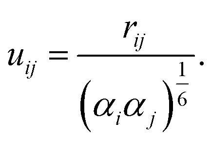
Taking advantage of this separation, an intramolecular potential was parametrized on energies, gradients, and multipoles (MBIS40) of isolated molecules on PBE0/def2-TZVP level of theory.41–43 For the treatment of intermolecular interactions, an additional separation of long-range and short-range interactions is introduced. We assume that long-range interactions, including electrostatics, polarization, and dispersion, are accurately captured by classical models using atomic multipoles and polarizabilities,44,45 and the D3 dispersion correction.46,47 As these descriptions break down at short distances, a number of classical models have been put forward in recent years,48,49 which resolve this limitation, for instance through the use of charge-penetration models for the description of short-range electrostatics.50 Here, a pairwise ML potential is adopted as an alternative. Within a classical formalism, potentials can be classified according to the information used as input feature (Fig. 1). We follow a classification based on two fundamental dimensions: the degree of directional information (angular momentum) and the number of particles (many-body order) involved in the interaction.
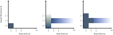 |
| | Fig. 1 Classification of classical intermolecular interactions. (left) Classical fixed-charge FF with point charges and a Lennard-Jones potential. (middle) Classical polarizable FF such as AMOEBA39 with the additional inclusion of polarization (∞, 1) and atomic multipoles (2, (0, 1, 2)). (right) Model proposed in this work, which includes a three-body dispersion term (3, 1) and a pairwise ML potential (2, (0, 1, 2)) compared to the polarizable FF. The pairwise ML potential can account for directional interactions in a systematic manner. | |
Thanks to their flexibility, ML potentials can be parametrized in a systematic manner according to the proposed categorization. In this work, we limit ourselves to an anisotropic pairwise ML potential, which is applied to intermolecular atom pairs at short distances in addition to dispersion, electrostatic, and polarization interactions. We will refer to this model as ANA2B, i.e., an anisotropic, non-additive FF in combination with a two-body ML potential.
As input features, pairwise distances, atom types, and the interaction coefficients of static and induced multipoles are used. A more detailed description of these features is given in Section 2.5.3. The pairwise intermolecular interaction is trained on neutral systems of the DES5M dataset,51 which includes intermolecular potentials of small molecule dimers obtained with spin-network-scaled MP2 (SNS-MP2).52–54 At present, DES5M is the largest dataset of high-quality intermolecular interactions. Since datasets of similar quality are not available for condensed-phase systems, we limit ourselves to DES5M for intermolecular interactions of dimers and PBE0/def2-TZVP for intramolecular interactions of monomers (see Section 2.5), with the aim to develop a model that can transfer from these small systems to the condensed phase.
2.2 Molecular graphs and atom types
The notion of atom types used as part of the proposed model relies on the formalism proposed in ref. 35. This formalism makes use of atom types, which are learned from molecular graphs, i.e., graphs that do not include information about the geometry of a molecule but only its covalent bonds. Graphs were constructed in the same manner as described in ref. 35. We will refer to these molecular graphs as  Atom types extracted from these molecular graphs are used as input features for subsequent tasks. The atom type of atom i is defined as an n-dimensional feature vector hin ∈ Rn where the superscript n indicates the order, i.e., h0 corresponds to the element itself, h1 to an atom type that incorporates information about the immediate neighbours, and so on. Atom types are learned as part of the training process with a message passing GNN as proposed in ref. 55.
2.3 Geometric graphs
The models for the prediction of atomic multipoles and the correction to the intramolecular potential VΔML use geometric information. These graphs were constructed by including an edge between all atoms, which were <5 Å apart. Following the approach described by Gasteiger et al.,56 distances were encoded with 20 Bessel functions and enveloped with a cutoff function to ensure a smooth cutoff. Element types were encoded as one-hot vectors serving as initial node features.
2.4 Message passing graph neural networks
Given a molecular or geometric graph  with nodes V and edges E as described above, message passing can be defined as,57,58
| | 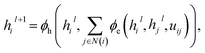 | (1) |
where hil ∈ Rn describes the hidden-feature vector of node vi after l iterations, uij ∈ Rn the edge feature of edge eij between node i and j, and N(i) denoting the set of neighbours of vi. ϕe and ϕh refer to edge and node update functions. The superscript l denotes the current message passing iteration. In this context, geometric and molecular graphs used in this work differ by the definition of N(i) and the edge feature uij.
2.5 Energy decomposition
Essential to the ANA2B model is a decomposition of interactions, which aims to follow a physically motivated classical description of interatomic interactions where possible. Remaining interactions are treated as corrections parametrized by ML models. The decomposition achieves two goals: first, the total potential energy is separated into manageable pieces. Second, the resulting interactions are interpretable. Here, a brief description of the involved interaction terms is given. Based on the classical description assumed in this work, interactions are separated into purely intermolecular and purely intramolecular contributions, as well as dispersion interactions (D3),| | | Vtotal = Vintra + Vinter + VD3. | (2) |
Dispersion interactions VD3 are described with the D3 dispersion correction46 using Becke–Johnson damping with parameters for PBE0,47,59 and are applied to both intramolecular and intermolecular interactions.
The purely intramolecular term Vintra is described in the ANA2B model by a ML potential, referred hereafter as VΔML. This ML potential was trained on energies and gradients of small molecules using PBE0/def2-TZVP as the reference method.
The purely intermolecular term Vinter consists of
| | | Vinter = VES + Vpol + VΔSR. | (3) |
where
Vpol refers to the polarization energy and
VΔSR to the short-range two-body ML correction. A detailed description of the intermolecular terms is given in the following paragraphs.
2.5.1 Electrostatics.
Long-range intermolecular electrostatic interactions are described with atomic multipoles. We made use of our previously introduced formalism for the prediction of atomic multipoles60 based on MBIS atomic multipoles40 up to the quadrupole and atomic volumes. Here, the model is re-trained and improved based on the model architecture described in ref. 61. Implementation of the electrostatic interaction and Ewald summation follows the formalism outlined in refs. 62–65. The interaction of point multipoles at site i and site j is decomposed in terms of order l,62| | 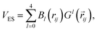 | (4) |
with multipole interaction coefficients Gl(![[r with combining right harpoon above (vector)]](https://www.rsc.org/images/entities/i_char_0072_20d1.gif) ij) and the radial functions Bl(rij) defined as62
ij) and the radial functions Bl(rij) defined as62| | 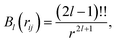 | (5) |
with !! refering to the double factorial. Note that intramolecular electrostatic interactions are contained in VΔML (see above).
2.5.2 Polarization.
A description of polarization is introduced through the Applequist model44 including Thole damping45 as the energy resulting from placing the molecule in the electric field produced by the static multipoles,| | 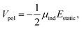 | (6) |
where μind refers to the self-consistently converged induced dipoles, and Estatic to the electric field produced by the static multipoles. Estatic is not damped and includes only intermolecular contributions. Induced dipoles μ are obtained asvia inversion of the 3N × 3N polarizability matrix B,66| | 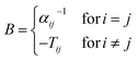 | (8) |
with the atomic polarizability αi and the elements Tij of the dipole–dipole interaction matrix. These elements Bij are damped with the damping proposed by Thole,| | | fThole = 1 − exp(−auij3) | (9) |
using a damping factor a and the polarizability-normalized distance| |  | (10) |
The damping factor a is set to 0.39 as in the AMOEBA FF.39 For the first order polarization model ANA2B1, μind was obtained as| | | μi,ind = αi × Ei,static, | (11) |
i.e., taking only the direct polarization into account. Thole damping is not applied to the direct polarization term. Periodic boundary conditions are introduced through the Ewald summation formalism described in ref. 67. The reciprocal space contribution is neglected for the mutual polarization term.
Static atomic dipole polarizabilities are obtained as
| | | αi = α0× 〈r3〉 × ϕα(hi2), | (12) |
where
α0 is the polarizability of the isolated element, and 〈
r3〉 the ratio between the atomic volume of the isolated atom and the atom in the molecule analogous to the Tkatchenko-Scheffler model.
68 Finally, an atom type derived scaling factor
ϕα(
hi2) is introduced to calibrate the polarizabilities with respect to the dataset published in ref.
69. Atomic volumes 〈
r3〉 are predicted by the same model that predicts the atomic multipoles,
i.e., for the isolated molecule using MBIS atomic volumes
40 as the reference.
2.5.3 Short-range correction (ΔSR).
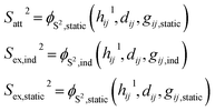
Instead of developing corrections for short-range phenomena such as charge penetration, a ML-parametrized pairwise interaction is proposed. This short-range pairwise potential is composed of the following terms,| | | VΔSR = Vex,static + Vex,ind + Vatt, | (13) |
and is applied to all intermolecular atom pairs within a distance of 6.5 Å.
The repulsive terms Vex,static and Vex,ind build on the orbital overlap model proposed by Salem70 and extended by Murrell et al.,71 which describes the exchange energy as a function of the orbital overlap S2,
| |  | (14) |
Attractive contributions to the short-range interaction due to charge transfer and charge-penetration effects are introduced as
Parameters for these interaction terms (coupling parameters
K and overlaps
S2) are parametrized by a ML model. The input features are described in the following.
• Pairwise atom types: features obtained from molecular graphs  described in Section 2.2 are symmetrized as hijl = ϕh(hil,hjl) + ϕh(hil,hjl). For the short-range correction, only first-order atom types are used. These will be referred to as hij1. Only first-order atom types are used to avoid overfitting as multipoles already include information about the environment.
• Distance features: distances are encoded with five Gaussians exp(−αrij2) with logarithmically spaced α ∈ 0.1, 1 Å−2. Preliminary work (data not shown) indicated that Bessel functions, which are frequently used to encode distances, induce oscillations in the pairwise potential. The Gaussians are centered at 0 to avoid this behaviour. These features will be referred to as dij.
• Anisotropic features: anisotropy is introduced based on the atomic multipoles Mk of order k as the symmetrized multipole–multipole interaction coefficients,62
| |  | (16) |
In this context, scalar multiplication is indicated by × and contractions are performed over the Cartesian components indicated by the greek indices.
ij,αβ refers to the tensor product of the Euclidean vector
ij,α =
j −
i with itself. Vectors
ij,α are normalized. Two types of features are used. The first type is calculated without inclusion of the induced dipoles,
i.e., (
M0,
M1,
M2), whereas the second includes the contribution of the induced dipoles,
i.e., (
M0,
M1 +
μind,
M2). These features will be referred to as
gij,static and
gij,ind, respectively.
Using the above features, the orbital overlaps S2 are parametrized by an artificial neural network (ANN) ϕS2 as,
| |  | (17) |
Overlaps sharing the same input features,
i.e.,
Satt2 and
Sex,static2, are predicted by the same model.
Coupling constants K are predicted as
that is without including the anisotropic features. Independent coupling constants are predicted for each term using the same model. Overlaps and Gaussian distance features are multiplied with a switching function to guarantee a smooth cutoff,
72| | 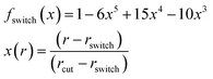 | (19) |
with distance
r, cutoff
rcut, and switching distance
rswitch. The switching distance is set to
rcut − 1 Å.
3. Methods
3.1 Models and training procedure
Several ML models were used in this work. An overview is given in Fig. 2. If not mentioned otherwise, ANN parametrized functions ϕ were constructed from two fully connected feed-forward layers of size 128 using the Swish activation function.73 The GNNs used to extract features of molecular graphs  employed a node-embedding and edge-embedding layer and message passing layers consisting of a single feed-forward layer of size 64. Each model was trained separately on its respective target. If not noted otherwise, models were optimized with Adam74 using an exponentially decaying learning rate ∈ [5 × 10⁻⁴, 1 × 10⁻⁵].
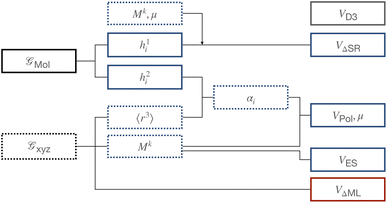 |
| | Fig. 2 Overview of the ANA2B model. Dotted lines refer to features that depend on the geometry while bold lines to features based on molecular graphs. Blue components refer to intermolecular interactions, red to intramolecular interactions, and grey to shared interactions. | |
3.1.1 Multipoles and atomic volumes.
MBIS multipoles on a PBE0/def2-TZVP level of theory were predicted using our previously introduced formalism for an equivariant multipole GNN.60 In addition, the MBIS atomic volume ratio was included. The message passing formalism described in ref. 60 was replaced with the AMP formalism described in ref. 61. For training, the dataset generated in ref. 60 was used and extended with conformations sampled with molecular dynamics (MD) to improve coverage of off-equilibrium conformations. MD simulations were performed with xTB (version 6.4.1)6 using the GFN-1 Hamiltonian.75 A seed conformation for MD was generated with the ETKDG conformation generator76 as implemented in the RDKit.77 MD simulations were carried out in the NVT ensemble for n × 100 ps, with integration steps of 0.5 fs at 800 K without any constraints. If not stated otherwise, default settings (sccacc = 2, hmass = 4 a.u.) were used. n was determined based on the number of heavy atoms in the molecule (<5: n = 16, <7: n = 8, <Z < 11: n = 4, >10: n = 2). Snapshots were written out every 100 ps. The n + 1 conformations, including the xTB GFN-1 minimum structure, obtained in this manner served as input for the following single-point calculations. Single-point gradients were evaluated for each structure with PBE0/def2-TZVP41–43 using PSI4 (version 1.4).78,79 MBIS multipoles40 and volumes were obtained with PSI4.80 If not stated otherwise, default PSI4 settings were used (energy and density convergence threshold 10−8 a.u.). Data for 1![[thin space (1/6-em)]](https://www.rsc.org/images/entities/char_2009.gif) 514462 conformations for a total of 451973 unique molecules were obtained in this way.
514462 conformations for a total of 451973 unique molecules were obtained in this way.
3.1.2 ML correction.
The ML correction was used to describe intramolecular interactions except for the contribution of the D3 dispersion model. The ΔML potential is based on the AMP architecture proposed in ref. 61. However, instead of a single set of multipoles, a total of 32 independent sets of multipoles up to the quadrupole were expanded on each atom. Note that these multipoles serve only as a tool to introduce directional interactions, unlike the electrostatic multipoles used for VES. Three message passing steps were employed with a cutoff of 5 Å. The model was trained over 2048 epochs on PBE0 potential energy and gradients. The model was trained on the same dataset used to train the multipole model. Gradient norms were clipped to norm 1. During each epoch, 1028 samples were presented. Each sample consisted of a batch of all conformations of five molecules. The model was trained on weighted relative energies and gradients,| |  | (20) |
ΔVML and ΔVref refer to the relative energies, i.e., the difference between the energy of a conformation i and a conformation j serving as a reference point ΔV = Vi − Vj. β was set to 0.9. Weights wi were defined as,| |  | (21) |
where Vmin is the energy of the conformation with the lowest energy of a given molecule, and N the numbers of atoms. T was set to 2000 K. Only molecules with more than one possible conformation and conformations with negative atomization energies and with maximum gradient components ≤2000 kJ mol−1 Å−1 were used.
3.1.3 Short-range correction.
The short-range pairwise potential VΔSR was trained on the intermolecular potentials of dimers in vacuum from the DES5M dataset.51 A cutoff of 6.5 Å was used for this interaction. As an exception, a cutoff of 5.5 Å was found to be optimal for the ANA2B0 model, i.e., the model without any polarization interactions. The model was trained over 512 epochs. Gradient norms were clipped to norm 1. During each epoch, 2048 samples were presented. Each sample consisted of all configurations of a given dimer. The mean squared error (MSE) between the predicted intermolecular potential and the reference (SNS-MP2)52,53 was optimized. Performance on the S7L81,82 and S66x8 (ref. 83) datasets were used as signals for early stopping. The mean absolute error (MAE) on a set of structures from X23 and ICE13 (CYTSIN01, URACIL, UREAXX12, HXMTAM10, CYHEXO, SUCACB03, CYANAM01, PYRZOL05, OXALAC04, ammonia, CO2 and ice polymorphs Ih and II) was used to the select the final models.
3.1.4 Polarizabilities.
The model used to predict polarizability scaling factors from molecular graphs was trained on a dataset of CCSD molecular polarizabilities reported in ref. 69. The model was trained over 512 epochs. During each epoch 512 randomly drawn samples consisting of a single molecule were presented. The model was optimized with respect to the MSE between the predicted molecular polarizability and the CCSD molecular polarizability.
3.2 General implementation details
All ML models were implemented in TensorFlow (version 2.11.0).84 The atomic simulation environment (ASE, version 3.22.1)85 was used as MD engine, for optimization, and for general analysis tasks including the calculation of harmonic free energies and thermodynamic integration. MDTraj (version 1.9.8)86 was used for post-processing and analysis tasks.
For long-range electrostatic interactions and polarization, a real-space cutoff of 10 Å was used. The screening parameter α for Ewald summations was set to 0.292 and 0.215 for the evaluation of the electrostatic interaction and the mutual polarization, respectively. Crystal structures were minimized with fixed lattice parameters. For MD simulations involving liquids, cutoffs for the D3 model were set to 10 Å, 5 Å, and 10 Å for the two-body-term, three-body-term, and the coordination number, respectively. For calculations and MD simulations involving crystals, cutoffs for the D3 model were set to 15 Å, 8 Å, and 15 Å for the two-body-term, three-body-term, and the coordination number, respectively.
3.3 Molecular dynamics (MD) set-up
Simulations of the pure liquids in the GROMOS 2016H66 dataset were performed with ASE.85 22 Å cubix boxes were generated with packmol87 followed by a pre-equilibration over 10000 steps at 300 K with OpenFF (version 2.0) using OpenMM (version 8.0).88,89 Equilibration and production runs were performed with an Andersen thermostat90 at the simulation temperature described in the GROMOS 2016H66 publication91 (298.15 K if not noted otherwise) and a Monte-Carlo barostat92 with a target pressure of 1 bar. The integration step was set to 0.5 fs. The equilibration was performed over 2000 steps (1 ps) using the respective ANA2B model with the collision frequency set to 0.1 and the barostat frequency set to 10. For the production run over 120000 steps (60 ps), the collision frequency was set to 0.01 and the barostat was applied every 25th step. These runs were repeated three times with different random number seeds for the generation of the initial velocities. Ensemble properties were averaged over the last 35 ps.
For the prediction of the heat of vaporization, monomers were simulated in the gas phase. These simulations were equilibrated over 2000 steps (1 ps) using a Berendsen thermostat93 (τ = 10 fs) followed by a 100000 step (50 ps) production run using a Langevin thermostat with a friction of 1 a.u. Starting conformations were generated with the ETKDG conformation generator76 in the RDKit.77 Averages were taken over four replicates with different initial velocities.
3.4 Ranking of crystal structures – CSP blind tests 3 and 5
For the third CSP blind test,94 all structures submitted by van Eijck were used (entries VIII, X, XI).95–97 For the fifth blind test,98 submissions of Neumann and co-workers were considered (entries XVI, XVII, XVIII).99–101 These submissions were selected because they contain in all cases a candidate structure that was considered a match with the experimental structure.
Candidate structures were relaxed under fixed lattices using the (L)BFGS optimizer with a tolerance of 1 kJ mol−1 Å−1.102–106 Lattices parameters were not minimized. Structures that did not converge within 250 steps were excluded.
3.5 Ranking of crystal structures – CSP blind test 6
3.5.1 Relaxation of crystal structures.
Lattices were relaxed with an external pressure of 1 bar using an anisotropic Monte Carlo barostat92 at 0 K. Subsequently, structures were relaxed under fixed lattices using the (L)BFGS optimizer with a tolerance of 1 kJ mol−1 Å−1.102–106
3.5.2 MD simulations.
The NPT ensemble was sampled using an Andersen thermostat90 and an anisotropic Monte Carlo barostat92 at 1 bar and a temperature of 150 K (XXII) and 300 (XXIII, XXVI). The collision frequency was set to 0.1 and the barostat frequency was set to 10. Structures were equilibrated for 1 ps followed by 5 ps production runs. These simulations were used to obtain thermally expanded cells and the mean potential energy.
3.5.3 Gibbs term.
The difference between the Helmholtz free energy F and the Gibbs free energy (G) was obtained as,107| | | ΔF→G = P〈V〉 + kBTlogρ(h|P,T), | (22) |
with 〈V〉 referring to the mean volume during the simulation and P to the pressure. The density ρ(h|P,T) was obtained through a kernel density estimation using Gaussian kernels with a width of 0.1. The density was estimated for the cell parameters.
3.5.4 Helmholtz free energy.
The harmonic Helmholtz free energy (FH) was calculated with the phonon module implemented in ASE using the minimized structures from step one. The phonon density of states was sampled on a uniform k-point grid of size (20, 20, 20) using 2000 sampling points.
3.5.5 Thermodynamic integration.
The anharmonic correction to the harmonic Helmholtz free energy (FA) was obtained with a thermodynamic integration from the harmonic potential (VH) to the unconstrained potential (VA),| |  | (23) |
following the description in ref. 108. The harmonic potential was obtained from the numerically calculated Hessian of the relaxed structure using the lattice parameters with the highest likelihood. The thermodynamic integration was performed over eleven uniformly spaced λ-points. Numerical integration was performed using a trapezoidal integration. An initial equilibration over 0.5 ps was performed followed by 0.1 ps of equilibration and 1 ps of sampling at each lambda point. The NVT ensemble was sampled with an Andersen thermostat90 at 150 K (XXII) and 300 K (XXIII, XXVI).
4 Results and discussion
The proposed ANA2B model was applied to a range of existing benchmarks to establish a level of accuracy. The datasets are categorized by their use as training, validation, or test set, and include intermolecular potential energies of dimers and lattice energies of molecular crystals and water ice. Particular attention is given to the role of polarization because preliminary results (data not shown) highlighted its importance. We have thus studied three variations of the ANA2B model: the first variation does not include any polarization interaction at all, and will be referred to as ANA2B0. The second variation, labelled ANA2B1, includes only the polarization stemming from the direct field, i.e., neglecting the mutual polarization. The third variation, labelled ANA2B∞, includes a full treatment of the direct and mutual polarization terms. At present, all models were only trained and applied to neutral molecules consisting of the elements H, C, N, O, F, S, Cl.
4.1 Monomers in vacuum
4.1.2 Performance on test set.
The following section reports the performance of the intramolecular ML potential on several computational benchmark datasets of conformation energies (Table 2). Overall, we find that our model performs comparable to the reference method (PBE0-D3BJ/def2-TZVP) with MAE values that are typically larger by a few tenths of a kJ mol−1. These results justify on one hand the decision to use the ML potential in place of the DFT calculation and that ML potentials might overall be able to substitute DFT in many situations. At the same time, datasets such as PCONF clearly display how the ML potential ‘inherits’ the accuracy of the method used to generate the training set.
Table 2 Mean absolute error (MAE) in [kJ mol−1] for the intramolecular ML potential used in this work for benchmarks of conformation energies (test sets). N is the number of data points per dataset. The method used to generate the training data (PBE0-D3) is shown as a comparison. More detailed error statistics is provided in Table S2 in the ESI
| Name |
N
|
Type |
Intra ML |
PBE0-D3 |
| Glucose109 |
205 |
Test |
2.5 |
2.3 |
| Maltose109 |
223 |
Test |
2.7 |
1.9 |
| SCONF110 |
17 |
Test |
1.6 |
1.1 |
| PCONF111 |
10 |
Test |
6.7 |
6.2 |
| ACONF112 |
15 |
Test |
0.5 |
0.2 |
| CYCONF113 |
15 |
Test |
2.7 |
2.7 |
4.2 Dimers in vacuum
4.2.2 Performance on validation set.
The S66x8 (ref. 83) and S7L81 datasets were used as early-stopping signal during training of the ANA2B models. While only small differences are found for the small molecule dimers in the S66x8 dataset, a considerably larger MAE is observed for the supramolecular systems in the S7L dataset. These results are consistent with the results observed for molecular systems shown below in Subsection 4.3. Very large molecules and/or molecular clusters might thus be an adequate and cost-efficient substitute to train and validate size-transferable ML potentials in the absence of condensed-phase data. For the S7L structures, the PNO coupled cluster calculations of ref. 82 were used (Table 4).
Table 4 Mean absolute error (MAE) in [kJ mol−1] for the validation sets S66x8 (ref. 83) and S7L.81,82N is the number of data points per dataset. More detailed error statistics is provided in Table S4 in the ESI
| Name |
N
|
Type |
ANA2B0 |
ANA2B1 |
ANA2B∞ |
| S66x8 (ref. 83) |
528 |
Validation |
1.3 |
0.8 |
0.8 |
| S7L81,82 |
7 |
Validation |
21.1 |
2.0 |
2.3 |
4.2.3 Performance on test set.
Table 5 lists MAE values for 14 computational benchmark datasets of dimer interaction potentials. In most cases, errors for the three ANA2B models are comparable. However, for datasets that contain highly polarizable systems, e.g., nucleobases in JSCH and ACHC, or for datasets with hydrogen-bonded systems, i.e., HB375x10, HB300SPXx10 and HBC1, the two models which include a treatment of polarization (ANA2B1 and ANA2B∞) perform better.
Table 5 Mean absolute error (MAE) in [kJ mol−1] for intermolecular potential benchmarks of dimers in vacuum (test sets). N is the number of data points per dataset. More detailed error statistics are provided in Tables S5–S7 in the ESI
| Name |
N
|
Type |
ANA2B0 |
ANA2B1 |
ANA2B∞ |
| SSI114 |
2596 |
Test |
0.6 |
0.7 |
0.6 |
| BBI114 |
100 |
Test |
1.0 |
0.7 |
0.7 |
| UBQ115 |
81 |
Test |
1.0 |
1.2 |
1.0 |
| ACHC8 |
54 |
Test |
4.8 |
2.2 |
1.0 |
| JSCH116 |
123 |
Test |
4.7 |
2.9 |
2.8 |
| HSG117 |
16 |
Test |
0.8 |
0.7 |
0.8 |
| HBC1 (ref. 118) |
58 |
Test |
8.5 |
3.3 |
2.0 |
| S22 (ref. 116) |
22 |
Test |
3.3 |
1.7 |
1.6 |
| S22x7 (ref. 119) |
154 |
Test |
5.9 |
3.0 |
2.8 |
| D1200 (ref. 120) |
482 |
Test |
1.7 |
1.2 |
1.2 |
| D442x10 (ref. 120) |
1570 |
Test |
1.9 |
1.6 |
1.5 |
| R739x5 (ref. 121) |
1615 |
Test |
2.5 |
2.3 |
2.3 |
| HB375x10 (ref. 122) |
3750 |
Test |
1.9 |
1.4 |
1.4 |
| HB300SPXx10 (ref. 123) |
1210 |
Test |
4.1 |
3.1 |
3.5 |
4.3 Molecular crystals
To assess whether the ANA2B can transfer from dimers and monomers in vacuum to condensed-phase systems, the model was applied to the prediction of lattice energies of molecular crystals. Table 6 and Fig. 3 show the corrected experimental lattice energies of the X23 dataset124–126 and diffusion Monte Carlo lattice energies for water ice polymorphs.127 Note that a subset of structures from X23 and ICE13 were used as validation structures to select the final model (see Section 3.1.3). Overall, the observed MAE is comparable to the most accurate dispersion corrected DFT calculations reported so far. For example, a recent study by Price et al.128 reported an MAE of 2.0 kJ mol−1 using B86bPBE-25 in combination with the XDM dispersion correction. The same study also reported an MAE of 0.8 kJ mol−1 for the ICE13 dataset. Note that direct comparison with B86bPBE-25 is somewhat complicated by the fact that the lattice energies were obtained for structures minimized with a different method (B86bPBE). Finally, the MAE for the X23 dataset with an existing multipole FF for molecular crystals, FIT,129 is reported as 9.2 kJ mol−1.130 This direct comparison indicates that the hybrid approach proposed in this work may present a way to unlock the full potential of classical FFs.
Table 6 Mean absolute error (MAE) in [kJ mol−1] for experimental (X23) and computationally (ICE13) derived lattice energies of molecular crystals in the test set. N is the number of data points per dataset. Results for B86bPBE and B86bPBE-25 with XDM dispersion correction are taken from ref. 128. B86bPBE-25 values were calculated with geometries relaxed at the B86bPBE level (B86bPBE-25//B86bPBE). 1Errors on a subset of X23 (cytosine, uracil, urea, hexamethylenetetramine, cyclohexane-1,4-dione, succinic acid, cyanamide, pyrazole, ammonia, and CO2) and ICE13 (ice Ih, ice II) were used to select the final model. Graphical results are shown in Fig. 3. More detailed error statistics are provided in Tables S8–S10 in the ESI
| Name |
N
|
Type |
ANA2B0 |
ANA2B1 |
ANA2B∞ |
B86bPBE |
B86bPBE-25 |
| X23 (ref. 124–126) |
23 |
Test1 |
4.6 |
3.2 |
2.9 |
3.0 |
2.0 |
| DMC-ICE13 (ref. 127) |
13 |
Test1 |
8.3 |
1.4 |
1.3 |
7.5 |
0.8 |
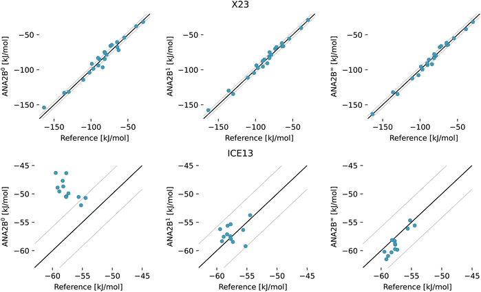 |
| | Fig. 3 Results for the lattice energies of systems in the X23 (top panels) and ICE13 datasets (bottom panels) with the ANA2B models. The left column (ANA2B0) refers to the model without any treatment of polarization, the middle (ANA2B1) column shows results for the model that includes only the direct polarization term, and the right column (ANA2B∞) displays results for the model which includes a full treatment of polarization. Equality ±4.184 kJ mol−1 is indicated by the black lines. | |
The overall good performance of ANA2B compared to hybrid DFT methods is particularly interesting considering that hybrid DFT calculations are currently probably the most accurate approach feasible for relatively large scale studies of condensed-phase systems. Taking into account the error of the reference method itself and the error resulting from the ML model underscores the importance of developing ML models, which are transferable and thus able to take advantage of the high-quality data available for small systems.
In the case of the ice polymorphs, the importance of a description of polarization becomes evident. While the expensive treatment of mutual polarization (ANA2B∞) results only in a small improvement of the MAE compared to the (ANA2B1), a clear difference is observed with regards to the ranking of the ice polymorphs (Table 6): for the ANA2B∞ model, good agreement with the DMC reference is found with a Spearman correlation coefficient rspearman of 0.77. For the ANA2B1, the ranking is considerably worse with a slightly negative coefficient rspearman = −0.04 (ANA2B0: rspearman = −0.74). While water presents a unique case, which might exaggerate the importance of polarization, these results still show a clear trend. Including some description of the non-additive nature of polarization might thus be the most important ingredient required to achieve transferability from vacuum to the condensed phase.
4.4 Condensed-phase properties of pure liquids
Prediction of experimental condensed-phase properties of molecular liquids have been a long-standing goal for the parametrization and testing of classical FF. Particularly for ML-based FF, these properties are an interesting test case as they require sufficient sampling in both the gas phase and the condensed phase.
Here, we rely on a dataset that was used to parametrize and validate the GROMOS 2016H66 FF.91 This dataset consists of a diverse set of 57 small molecules and several properties including the heat of vaporization, density (ρ), isothermal compressibility (κ), thermal expansion coefficient (α), and the dielectric permittivity (ε). We limit the analysis to the heat of vaporization and the density in this study due to the slow convergence of the other properties. Results with ANA2B1 are shown in Table 7. For both properties, we observe RMSE values comparable to the fixed-charge FFs (IPA and GROMOS 2016H66) shown in Fig. 4 and Table 7, confirming the observation made for the prediction of lattice energies, i.e., transferability to the condensed phase is possible for the ANA2B1 model. These results are particularly noteworthy as GROMOS 2016H66 was parametrized on these two thermodynamic properties. The slightly smaller error of IPA for the density might stem from the fact that its parametrization included molecular crystals, indicating that the prediction of densities could be improved by incorporating condensed-phase structures during training. Finally, we note that as the only exception, two of three simulations of ethylenediamine in the liquid phase crashed after 24.3 and 31.6 ps, respectively, with the ANA2B1 model.
Table 7 Root-mean-square error (RMSE) for pure liquid properties of 57 systems used in the calibration and validation of the GROMOS 2016H66 FF91 for the ANA2B1 model. Values for GROMOS 2016H66 and IPA were taken from the referenced publications. The uncertainty is given as the mean standard deviation obtained over four replicates. More detailed error statistics is provided in Table S11 in the ESI. The individual numerical values are given in Table S12
| Property |
IPA35 |
GROMOS 2016H66 (ref. 91) |
ANA2B1 |
|
H
vap [kJ mol−1] |
4.5 |
3.5 |
2.8 ± 0.9 |
|
ρ [kg m−3] |
26.3 |
32.4 |
33.9 ± 5.8 |
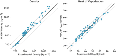 |
| | Fig. 4 Results for condensed-phase properties of 57 molecules used in the parametrization and validation of GROMOS 2016H66: density (left) and heat of vaporization (right) for the ANA2B1 model. Black lines indicate equality ±50 kg m−3 and ±4.184 kJ mol−1. | |
4.5 Crystal structure prediction
Having established a level of accuracy in the previous sections, this last section is concerned with the application of the ANA2B∞ model to the (retrospective) ranking of molecular crystals. As targets we use the structures, which were part of the CSP blind tests 3,94 5,98 and 6 (ref. 29) organized by the Cambridge Crystallographic Data Centre in the past. These blind tests were chosen due to the availability of all submitted candidates, allowing for the least biased assessment of the ability to find the experimental crystal structure given a list of candidates. We limit ourselves to the pure and neutral targets restricted to H, C, N, O, F, S, Cl. Target XX of the third blind test was excluded due to convergence issues. For the third and fifth blind test, a ranking based on lattice energies is used. For the sixth blind test, we furthermore explore how additional contributions, such as entropic terms, impact the ranking.
4.5.1 CSP blind tests 3 and 5.
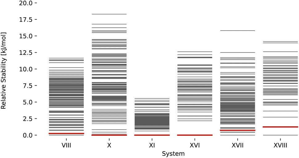
Rankings for targets stemming from the third and fifth blind test are shown in Fig. 5. Candidates for blind test three submitted by van Eijck were generated using random search.96 Candidates for the fifth blind test submitted by Neumann et al. were generated using Monte Carlo parallel tempering.100 In all cases, a match with the experimental structure (red) would have been found as the most stable structure within a window of <1.3 kJ mol−1. Overall, these results underscore the strength of the proposed ML-augmented FF, which yields rankings that are in most cases comparable to rankings based on much more expensive methods such as system-tailored FFs101 or DFT.131
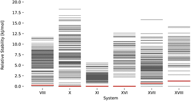 |
| | Fig. 5 Stability ranking for the crystal structure for the compounds of the CSP blind tests 3 (VIII, X, XI)94 and 5 (XVI, XVII, XVIII)98 using the lattice energy predicted with the ANA2B∞ model. Each horizontal bar represents the stability of a structure with respect to the most stable structure. Red bars indicate experimental structures. The candidate structures were taken from the corresponding publications.94,98 | |
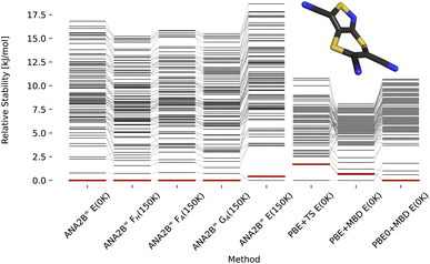
4.5.2 CSP blind test 6.
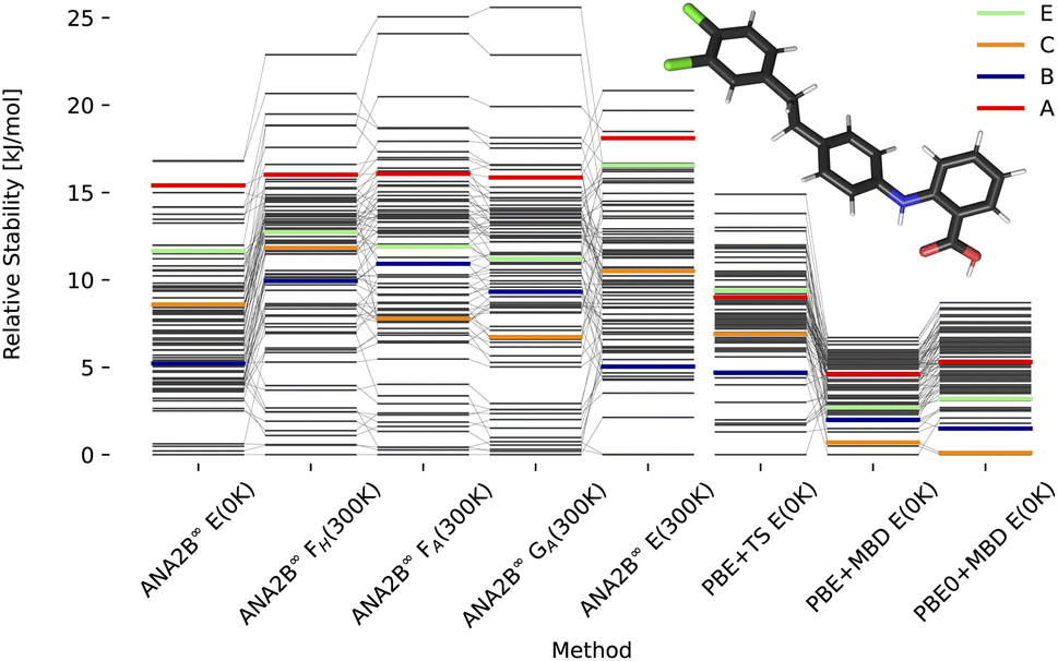
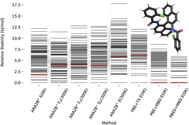
In previous work, Hoja et al.31 presented a workflow to rank crystal structures of the 6th CSP blind test29 in a hierarchical manner. They generated candidate structures first using the tailor-made FF developed by Neumann and co-workers,100,101 and subsequently ranked them with increasingly computationally demanding methods, including vibrational contributions in the final ranking. Here, we base our study on the candidate structures made available as part of their work,31 which includes all known experimental structures. The exhaustive computational study by Hoja et al. has provided insight into the different contributions stemming from DFT on different levels of theory and vibrational contributions, which we can use for a comparison with our ANA2B∞ model. Rankings for the three pure systems XXII, XXIII, and XXVI are shown in Fig. 6–8 based on the lattice energy (ANA2B∞E(0 K)), the harmonic Helmholtz free energy (ANA2B∞FH(T)), the Helmholtz free energy including anharmonic corrections (ANA2B∞FA(T)), the Gibbs free energy (ANA2B∞GA(T), and the mean potential energy during a molecular simulation (ANA2B∞E(T)). Rankings for dispersion corrected PBE and PBE0 are taken from ref. 31.
 |
| | Fig. 6 Stability ranking for the crystal structure of compound XXII. Each horizontal bar represents the stability of a structure with respect to the most stable structure. The stability is given in kJ per mol per molecule. Candidate structures and rankings for dispersion corrected PBE and PBE0 are taken from ref. 31. Experimental structures are marked in red. | |
 |
| | Fig. 7 Stability ranking for the crystal structure of compound XXIII. Each horizontal bar represents the stability of a structure with respect to the most stable structure. The stability is given in kJ per mol per molecule. Candidate structures and rankings for dispersion corrected PBE and PBE0 are taken from ref. 31. Experimental structures are marked in color. | |
 |
| | Fig. 8 Stability ranking for the crystal structure of compound XXVI. Each horizontal bar represents the stability of a structure with respect to the most stable structure. The stability is given in kJ per mol per molecule. Candidate structures and rankings for dispersion corrected PBE and PBE0 are taken from ref. 31. Experimental structures are marked in red. Note that PBE0 + MBD is not available for all polymorphs of this structure. | |
For compounds XXII and XXVI, the ANA2B∞ lattice energy ranks the experimental polymorph as the most stable (XXII) and the fifth most stable (XXVI) structure within a window of 2 kJ mol−1. Interestingly, we do not observe a distinct benefit for the inclusion of corrections to the lattice energy based on entropic contributions. While in some cases a destabilization of non-experimental structures is observed, no systematic improvement of the actual ranking is found. This surprising finding suggests that improving the accuracy of the predicted energy might be the highest priority for future work. A fine-tuning on high-quality data of crystalline energies and/or gradients could be a possible solution. Such a fine-tuning might be particularly important for systems where a fine balance between intramolecular and intermolecular interactions exists, i.e., most flexible molecules.
A second interesting observation concerns compound XXIII, where the ANA2B∞ model fails to rank the experimental structures near the most stable candidate. This failure is most evident for polymorph A, which is in all cases ranked as one of the least stable structures. As the only exception, polymorph B is found within a window of a bit more than 5 kJ mol−1. Importantly, several structures, most notably polymorph D and N70, could not be converged during the optimization or resulted in unstable MD simulations. In previous work,31 N70 was ranked as the most stable polymorph with PBE0 + MBD + Fvib.
Relative errors in percent of the lattice cell parameters with respect to the experimental structures are given in Table 8. A consistent underestimation of cell parameters and volumes is found, consistent with the results obtained for the densities of liquids. However, unlike for liquids sampled at finite temperatures, the underestimation of cell volumes might be explained partially with the optimization of cell parameters at 0 K.
Table 8 Relative deviations in percentage ((pred. − exp.)/exp.) × 100%) from the experimental lattice cell parameters and volumes for the polymorphs minimized with ANA2B∞ and mean absolute percentage errors (MAPE)
| Systems |
a
|
b
|
c
|
α
|
β
|
γ
|
Volume |
| XXII-N2 |
−0.78 |
−0.49 |
1.11 |
— |
0.76 |
— |
−0.66 |
| XXIII-A |
−1.85 |
−2.45 |
0.37 |
— |
−1.48 |
— |
−3.69 |
| XXIII-B |
2.55 |
−0.49 |
−4.92 |
3.97 |
1.56 |
−1.49 |
−3.47 |
| XXIII-C |
−2.70 |
−0.81 |
−0.92 |
2.03 |
2.06 |
0.23 |
−3.96 |
| XXIII-D |
−2.20 |
0.63 |
0.99 |
— |
2.07 |
— |
−2.47 |
| XXVI-N1 |
−1.72 |
−1.26 |
−2.64 |
3.30 |
0.73 |
0.86 |
−4.41 |
| MAPE |
1.97 |
1.02 |
1.83 |
3.10 |
1.44 |
0.86 |
3.11 |
5 Conclusion
In the present work, we have introduced a hybrid classical/ML potential for the simulation of molecular systems. Our work demonstrates that the combination of classical potentials with specific ML-based corrections can result in highly accurate, interpretable, and transferable potentials. The classical description of atomic interactions can thereby profit from augmentation with ML while ML can profit from the constraints imposed by classical models, especially for long-range interactions (such as dispersion, electrostatics, and polarization). The proposed hybrid approach could thus fill the existing methodological gap with a method, which can reach the accuracy of DFT at a computational cost between classical FF and semi-empirical methods while simultaneously improving the applicability of ML potentials. In the present work, particular attention was given to the development of an ML-based approach, which can be used for condensed-phase systems but does not require reference data of such systems. Our results indicate that such an approach could be a powerful tool for crystal structure prediction, in particular. System-specific fine-tuning could further improve structural rankings and render FFs a viable choice for crystal structure prediction tasks.
Besides improving the efficiency and computational cost, possible avenues for future investigations could include the explicit treatment of three-body interactions with a ML potential or higher-order polarization. However, both of these options would result in significant additional computational costs. An alternative route might be the application within a semi-empirical model instead of a classical FF. In principle, the proposed pairwise ML potential could be applied to semi-empirical methods. Assuming that semi-empirical methods are able to accurately describe long-range interactions, a short-range pairwise potential might be able to largely resolve the limitations of semi-empirical models. This application might be particularly interesting for systems for which the classical approximations assumed in this work are not valid. In a similar vein, the pairwise potential could also be used to improve the description interactions between the QM and MM particles in QM/MM simulations, which typically still rely on classical Lennard-Jones potentials.
Overall, we anticipate that the proposed methods will significantly facilitate the parametrization of highly accurate FF.
Data availability
All datasets used in this work are publicly available (see the corresponding references in the text). The dataset used to train the intramolecular potential is published as part of this work and can be found on the ETH Research Collection https://www.research-collection.ethz.ch/handle/20.500.11850/626683 Code and model weights necessary to reproduce the results in this work are made available on GitHub: https://github.com/rinikerlab/ANA2B.
Author contributions
M. T.: conceptualization, data generation and curation, methodology, software, validation, visualization, writing – original draft. S. R.: conceptualization, funding acquisition, methodology, project administration, resources, supervision, writing – review and editing.
Conflicts of interest
There are no conflicts to declare.
Acknowledgements
The authors thank Felix Pultar for helpful discussions.
Notes and references
- M. Del Ben, M. Schönherr, J. Hutter and J. VandeVondele, J. Phys. Chem. Lett., 2013, 4, 3753–3759 Search PubMed
 .
.
- M. Chen, H.-Y. Ko, R. C. Remsing, M. F. C. Andrade, B. Santra, Z. Sun, A. Selloni, R. Car, M. L. Klein, J. P. Perdew and X. Wu, Proc. Natl. Acad. Sci. U. S. A., 2017, 114, 10846–10851 Search PubMed .
- N. Schuch and F. Verstraete, Nat. Phys., 2009, 5, 732–735 Search PubMed .
- S. Riniker, J. Chem. Inf. Model., 2018, 58, 565–578 Search PubMed .
-
J. A. Pople and D. L. Beveridge, Approximate Molecular Orbital Theory, McGraw-Hill, 1970 Search PubMed .
- C. Bannwarth, E. Caldeweyher, S. Ehlert, A. Hansen, P. Pracht, J. Seibert, S. Spicher and S. Grimme, WIREs, 2021, 11, e1493 Search PubMed .
-
D. E. Shaw, P. J. Adams, A. Azaria, J. A. Bank, B. Batson, A. Bell, M. Bergdorf, J. Bhatt, J. A. Butts, T. Correia, R. M. Dirks, R. O. Dror, M. P. Eastwood, B. Edwards, A. Even, P. Feldmann, M. Fenn, C. H. Fenton, A. Forte, J. Gagliardo, G. Gill, M. Gorlatova, B. Greskamp, J. Grossman, J. Gullingsrud, A. Harper, W. Hasenplaugh, M. Heily, B. C. Heshmat, J. Hunt, D. J. Ierardi, L. Iserovich, B. L. Jackson, N. P. Johnson, M. M. Kirk, J. L. Klepeis, J. S. Kuskin, K. M. Mackenzie, R. J. Mader, R. McGowen, A. McLaughlin, M. A. Moraes, M. H. Nasr, L. J. Nociolo, L. O'Donnell, A. Parker, J. L. Peticolas, G. Pocina, C. Predescu, T. Quan, J. K. Salmon, C. Schwink, K. S. Shim, N. Siddique, J. Spengler, T. Szalay, R. Tabladillo, R. Tartler, A. G. Taube, M. Theobald, B. Towles, W. Vick, S. C. Wang, M. Wazlowski, M. J. Weingarten, J. M. Williams and K. A. Yuh, Proceedings of the International Conference for High Performance Computing, Networking, Storage and Analysis, 2021 Search PubMed .
- T. M. Parker and C. D. Sherrill, J. Chem. Theory Comput., 2015, 11, 4197–4204 Search PubMed .
- H. E. Sauceda, M. Gastegger, S. Chmiela, K.-R. Müller and A. Tkatchenko, J. Chem. Phys., 2020, 153, 124109 Search PubMed .
- J. Behler, J. Chem. Phys., 2011, 134, 074106 Search PubMed .
- K. T. Schütt, H. E. Sauceda, P.-J. Kindermans, A. Tkatchenko and K.-R. Müller, J. Chem. Phys., 2018, 148, 241722 Search PubMed .
- A. P. Bartók, S. De, C. Poelking, N. Bernstein, J. R. Kermode, G. Csányi and M. Ceriotti, Sci. Adv., 2017, 3, e1701816 Search PubMed .
- O. T. Unke, S. Chmiela, H. E. Sauceda, M. Gastegger, I. Poltavsky, K. T. Schütt, A. Tkatchenko and K.-R. Müller, Chem. Rev., 2021, 121, 10142–10186 Search PubMed .
- S. Chmiela, A. Tkatchenko, H. E. Sauceda, I. Poltavsky, K. T. Schütt and K.-R. Müller, Sci. Adv., 2017, 3, e1603015 Search PubMed .
- J. Gasteiger, F. Becker and S. Günnemann, Adv. Neural Inf. Process. Syst., 2021, 34, 6790–6802 Search PubMed .
- O. T. Unke, S. Chmiela, M. Gastegger, K. T. Schütt, H. E. Sauceda and K.-R. Müller, Nat. Commun., 2021, 12, 7273 Search PubMed .
-
K. T. Schütt, O. T. Unke and M. Gastegger, International Conference on Machine Learning, 2021, pp. 9377–9388 Search PubMed .
- A. Musaelian, S. Batzner, A. Johansson, L. Sun, C. J. Owen, M. Kornbluth and B. Kozinsky, Nat. Commun., 2023, 14, 579 Search PubMed .
-
I. Batatia, D. P. Kovács, G. N. Simm, C. Ortner and G. Csányi, Advances in Neural Information Processing Systems, 2022, vol. 35, pp. 11423–11436 Search PubMed .
-
I. Batatia, S. Batzner, D. P. Kovács, A. Musaelian, G. N. Simm, R. Drautz, C. Ortner, B. Kozinsky and G. Csányi, arXiv, 2022, preprint, arXiv:2205.06643, DOI:10.48550/arXiv.2205.06643.
- S. Stocker, J. Gasteiger, F. Becker, S. Günnemann and J. T. Margraf, Mach. Learn.: Sci. Technol., 2022, 3, 045010 Search PubMed .
- I. Poltavsky and A. Tkatchenko, J. Phys. Chem. Lett., 2021, 12, 6551–6564 Search PubMed .
- J. Daru, H. Forbert, J. Behler and D. Marx, Phys. Rev. Lett., 2022, 129, 226001 Search PubMed .
-
J. Lan, D. Wilkins, V. Rybkin, M. Iannuzzi and J. Hutter, ChemRxiv, 2021, preprint, chemrxiv–2021–n32q8–v2.
-
A. R. Oganov, Modern Methods of Crystal Structure Prediction, John Wiley & Sons, 2011 Search PubMed .
-
S. Atahan-Evrenk and A. Aspuru-Guzik, Prediction and Calculation of Crystal Structures, Springer, 2014 Search PubMed .
- S. Woodley and R. Catlow, Nature Mater., 2008, 7, 937–946 Search PubMed .
- S. L. Price, Chem. Soc. Rev., 2014, 43, 2098–2111 Search PubMed .
- A. M. Reilly, R. I. Cooper, C. S. Adjiman, S. Bhattacharya, A. D. Boese, J. G. Brandenburg, P. J. Bygrave, R. Bylsma, J. E. Campbell, R. Car, D. H. Case, R. Chadha, J. C. Cole, K. Cosburn, H. M. Cuppen, F. Curtis, G. M. Day, R. A. DiStasio Jr, A. Dzyabchenko, B. P. van Eijck, D. M. Elking, J. A. van den Ende, J. C. Facelli, M. B. Ferraro, L. Fusti-Molnar, C.-A. Gatsiou, T. S. Gee, R. de Gelder, L. M. Ghiringhelli, H. Goto, S. Grimme, R. Guo, D. W. M. Hofmann, J. Hoja, R. K. Hylton, L. Iuzzolino, W. Jankiewicz, D. T. de Jong, J. Kendrick, N. J. J. de Klerk, H.-Y. Ko, L. N. Kuleshova, X. Li, S. Lohani, F. J. J. Leusen, A. M. Lund, J. Lv, Y. Ma, N. Marom, A. E. Masunov, P. McCabe, D. P. McMahon, H. Meekes, M. P. Metz, A. J. Misquitta, S. Mohamed, B. Monserrat, R. J. Needs, M. A. Neumann, J. Nyman, S. Obata, H. Oberhofer, A. R. Oganov, A. M. Orendt, G. I. Pagola, C. C. Pantelides, C. J. Pickard, R. Podeszwa, L. S. Price, S. L. Price, A. Pulido, M. G. Read, K. Reuter, E. Schneider and C. Schob, Acta. Crystallogr., B, 2016, 72, 439–459 Search PubMed .
- J. Nyman and G. M. Day, Cryst. Eng. Comm., 2015, 17, 5154–5165 Search PubMed .
- J. Hoja, H.-Y. Ko, M. A. Neumann, R. Car, R. A. DiStasio and A. Tkatchenko, Sci. Adv., 2019, 5, eaau3338 Search PubMed .
- M. Rossi, P. Gasparotto and M. Ceriotti, Phys. Rev. Lett., 2016, 117, 115702 Search PubMed .
- V. Kapil and E. A. Engel, Proc. Natl. Acad. Sci. U. S. A., 2022, 119, e2111769119 Search PubMed .
- A. M. Alvertis and E. A. Engel, Phys. Rev. B, 2022, 105, L180301 Search PubMed .
- M. Thürlemann, L. Böselt and S. Riniker, J. Chem. Theory Comput., 2023, 19, 562–579 Search PubMed .
- A. McSloy, G. Fan, W. Sun, C. Hölzer, M. Friede, S. Ehlert, N.-E. Schütte, S. Grimme, T. Frauenheim and B. Aradi, J. Chem. Phys., 2023, 158, 034801 Search PubMed .
- M. F. Kasim and S. M. Vinko, Phys. Rev. Lett., 2021, 127, 126403 Search PubMed .
- S. Schoenholz and E. D. Cubuk, Adv. Neural Inf. Process. Syst., 2020, 33, 11428–11441 Search PubMed .
- J. W. Ponder, C. Wu, P. Ren, V. S. Pande, J. D. Chodera, M. J. Schnieders, I. Haque, D. L. Mobley, D. S. Lambrecht, R. A. DiStasio, M. Head-Gordon, G. N. I. Clark, M. E. Johnson and T. Head-Gordon, J. Phys. Chem. B, 2010, 114, 2549–2564 Search PubMed .
- T. Verstraelen, S. Vandenbrande, F. Heidar-Zadeh, L. Vanduyfhuys, V. Van Speybroeck, M. Waroquier and P. W. Ayers, J. Chem. Theory Comput., 2016, 12, 3894–3912 Search PubMed .
- C. Adamo and V. Barone, J. Chem. Phys., 1999, 110, 6158–6170 Search PubMed .
- J. P. Perdew, K. Burke and M. Ernzerhof, Phys. Rev. Lett., 1996, 77, 3865–3868 Search PubMed .
- F. Weigend and R. Ahlrichs, Phys. Chem. Chem. Phys., 2005, 7, 3297–3305 Search PubMed .
- J. Applequist, J. R. Carl and K.-K. Fung, J. Am. Chem. Soc., 1972, 94, 2952–2960 Search PubMed .
- B. Thole, Chem. Phys., 1981, 59, 341–350 Search PubMed .
- S. Grimme, J. Antony, S. Ehrlich and H. Krieg, J. Chem. Phys., 2010, 132, 154104 Search PubMed .
- S. Grimme, S. Ehrlich and L. Goerigk, J. Comput. Chem., 2011, 32, 1456–1465 Search PubMed .
- J. A. Rackers, R. R. Silva, Z. Wang and J. W. Ponder, J. Chem. Theory Comput., 2021, 17, 7056–7084 Search PubMed .
- J. A. Rackers and J. W. Ponder, J. Chem. Phys., 2019, 150, 084104 Search PubMed .
- J. A. Rackers, Q. Wang, C. Liu, J.-P. Piquemal, P. Ren and J. W. Ponder, Phys. Chem. Chem. Phys., 2017, 19, 276–291 Search PubMed .
- A. G. Donchev, A. G. Taube, E. Decolvenaere, C. Hargus, R. T. McGibbon, K.-H. Law, B. A. Gregersen, J.-L. Li, K. Palmo, K. Siva, M. Bergdorf, J. L. Klepeis and D. E. Shaw, Sci. Data, 2021, 8, 55 Search PubMed .
- R. T. McGibbon, A. G. Taube, A. G. Donchev, K. Siva, F. Hernández, C. Hargus, K.-H. Law, J. L. Klepeis and D. E. Shaw, J. Chem. Phys., 2017, 147, 161725 Search PubMed .
- S. Grimme, J. Chem. Phys., 2003, 118, 9095–9102 Search PubMed .
- C. Möller and M. S. Plesset, Phys. Rev., 1934, 46, 618–622 Search PubMed .
- P. W. Battaglia, R. Pascanu, M. Lai, D. J. Rezende and K. Kavukcuoglu, Adv. Neural Inf. Process. Syst., 2016, 4509–4517 Search PubMed .
-
J. Klicpera, J. Groß and S. Günnemann, arXiv, 2020, preprint, arXiv:2003.03123, DOI:10.48550/arXiv.2003.03123.
-
J. Gilmer, S. S. Schoenholz, P. F. Riley, O. Vinyals and G. E. Dahl, International Conference on Machine Learning, 2017, pp. 1263–1272 Search PubMed .
-
P. W. Battaglia, J. B. Hamrick, V. Bapst, A. Sanchez-Gonzalez, V. F. Zambaldi, M. Malinowski, A. Tacchetti, D. Raposo, A. Santoro, R. Faulkner, Ç. Gülçehre, H. F. Song, A. J. Ballard, J. Gilmer, G. E. Dahl, A. Vaswani, K. R. Allen, C. Nash, V. Langston, C. Dyer, N. Heess, D. Wierstra, P. Kohli, M. Botvinick, O. Vinyals, Y. Li and R. Pascanu, arXiv, 2018, preprint, arXiv:1806.01261 Search PubMed.
- E. R. Johnson and A. D. Becke, J. Chem. Phys., 2005, 123, 024101 Search PubMed .
- M. Thürlemann, L. Böselt and S. Riniker, J. Chem. Theory Comput., 2022, 18, 1701–1710 Search PubMed .
-
M. Thürlemann and S. Riniker, Anisotropic message passing: graph neural networks with directional and long-range interactions, in International Conference on Learning Representations, 2023 Search PubMed .
- C. J. Burnham and N. J. English, Int. J. Mol. Sci., 2020, 21, 277 Search PubMed .
-
W. Smith, Information Newsletter for Computer Simulation of Condensed Phases, 1998, pp. 15–25 Search PubMed .
- D. Lin, J. Chem. Phys., 2015, 143, 114115 Search PubMed .
- J. Stenhammar, M. Trulsson and P. Linse, J. Chem. Phys., 2011, 134, 224104 Search PubMed .
-
A. Stone, The Theory of Intermolecular Forces, Oxford University Press, 2013 Search PubMed .
- L. Lagardère, F. Lipparini, E. Polack, B. Stamm, E. Cancèès, M. Schnieders, P. Ren, Y. Maday and J.-P. Piquemal, J. Chem. Theory Comput., 2015, 11, 2589–2599 Search PubMed .
- A. Tkatchenko and M. Scheffler, Phys. Rev. Lett., 2009, 102, 073005 Search PubMed .
- Y. Yang, K. U. Lao, D. M. Wilkins, A. Grisafi, M. Ceriotti and R. A. DiStasio, Sci. Data, 2019, 6, 152 Search PubMed .
- L. Salem and H. C. Longuet-Higgins, Proc. R. Soc. Lond., 1961, 264, 379–391 Search PubMed .
- J. N. Murrell, M. Randic, D. R. Williams and H. C. Longuet-Higgins, Proc. R. Soc. Lond., 1965, 284, 566–581 Search PubMed .
- J. Guenot and P. A. Kollman, J. Comp. Chem., 1993, 14, 295–311 Search PubMed .
-
P. Ramachandran, B. Zoph and Q. V. Le, arXiv, 2017, preprint, arXiv:1710.05941, DOI:10.48550/arXiv.1710.05941.
-
D. P. Kingma and J. Ba, arXiv, 2017, preprint, arXiv:1412.6980, DOI:10.48550/arXiv.1412.6980.
- S. Grimme, C. Bannwarth and P. Shushkov, J. Chem. Theory Comput., 2017, 13, 1989–2009 Search PubMed .
- S. Riniker and G. A. Landrum, J. Chem. Inf. Model., 2015, 55, 2562–2574 Search PubMed .
-
G. Landrum, P. Tosco, B. Kelley, sriniker, ric, gedeck, R. Vianello, N. Schneider, A. Dalke, D. N. E. Kawashima, B. Cole, S. Turk, M. Swain, A. Savelyev, D. Cosgrove, A. Vaucher, M. Wójcikowski, D. Probst, G. Godin, G. Jones, V. F. Scalfani, A. Pahl, F. Berenger, J. L. Varjo, strets123, J. P. Doliath Gavid, G. Sforna and J. H. Jensen, rdkit/rdkit: 2020_09_5 (Q3 2020) Release, 2021 Search PubMed .
- J. M. Turney, A. C. Simmonett, R. M. Parrish, E. G. Hohenstein, F. A. Evangelista, J. T. Fermann, B. J. Mintz, L. A. Burns, J. J. Wilke, M. L. Abrams, N. J. Russ, M. L. Leininger, C. L. Janssen, E. T. Seidl, W. D. Allen, H. F. Schaefer, R. A. King, E. F. Valeev, C. D. Sherrill and T. D. Crawford, Wiley Interdiscip. Rev.: Comput. Mol. Sci., 2012, 2, 556–565 Search PubMed .
- R. M. Parrish, L. A. Burns, D. G. A. Smith, A. C. Simmonett, A. E. DePrince, E. G. Hohenstein, U. Bozkaya, A. Y. Sokolov, R. Di Remigio, R. M. Richard, J. F. Gonthier, A. M. James, H. R. McAlexander, A. Kumar, M. Saitow, X. Wang, B. P. Pritchard, P. Verma, H. F. Schaefer, K. Patkowski, R. A. King, E. F. Valeev, F. A. Evangelista, J. M. Turney, T. D. Crawford and C. D. Sherrill, J. Chem. Theory Comput., 2017, 13, 3185–3197 Search PubMed .
- D. G. A. Smith, L. A. Burns, A. C. Simmonett, R. M. Parrish, M. C. Schieber, R. Galvelis, P. Kraus, H. Kruse, R. Di Remigio, A. Alenaizan, A. M. James, S. Lehtola, J. P. Misiewicz, M. Scheurer, R. A. Shaw, J. B. Schriber, Y. Xie, Z. L. Glick, D. A. Sirianni, J. S. O'Brien, J. M. Waldrop, A. Kumar, E. G. Hohenstein, B. P. Pritchard, B. R. Brooks, H. F. Schaefer, A. Y. Sokolov, K. Patkowski, A. E. DePrince, U. Bozkaya, R. A. King, F. A. Evangelista, J. M. Turney, T. D. Crawford and C. D. Sherrill, J. Chem. Phys., 2020, 152, 184108 Search PubMed .
- R. Sedlak, T. Janowski, M. Pitonák, J. Rezác, P. Pulay and P. Hobza, J. Chem. Theory Comput., 2013, 9, 3364–3374 Search PubMed .
- Y. S. Al-Hamdani, P. R. Nagy, A. Zen, D. Barton, M. Kállay, J. G. Brandenburg and A. Tkatchenko, Nat. Commun., 2021, 12, 3927 Search PubMed .
- J. Rezàc, K. E. Riley and P. Hobza, J. Chem. Theory Comput., 2011, 7, 3466–3470 Search PubMed .
-
M. Abadi, A. Agarwal, P. Barham, E. Brevdo, Z. Chen, C. Citro, G. S. Corrado, A. Davis, J. Dean, M. Devin, S. Ghemawat, I. Goodfellow, A. Harp, G. Irving, M. Isard, Y. Jia, R. Jozefowicz, L. Kaiser, M. Kudlur, J. Levenberg, D. Mane, R. Monga, S. Moore, D. Murray, C. Olah, M. Schuster, J. Shlens, B. Steiner, I. Sutskever, K. Talwar, P. Tucker, V. Vanhoucke, V. Vasudevan, F. Viegas, O. Vinyals, P. Warden, M. Wattenberg, M. Wicke, Y. Yu and X. Zheng, arXiv, 2016, preprint, arXiv:1603.04467, DOI:10.48550/arXiv.1603.04467.
- A. H. Larsen, J. J. Mortensen, J. Blomqvist, I. E. Castelli, R. Christensen, M. Dulak, J. Friis, M. N. Groves, B. Hammer, C. Hargus, E. D. Hermes, P. C. Jennings, P. B. Jensen, J. Kermode, J. R. Kitchin, E. L. Kolsbjerg, J. Kubal, K. Kaasbjerg, S. Lysgaard, J. B. Maronsson, T. Maxson, T. Olsen, L. Pastewka, A. Peterson, C. Rostgaard, J. Schiotz, O. Schütt, M. Strange, K. S. Thygesen, T. Vegge, L. Vilhelmsen, M. Walter, Z. Zeng and K. W. Jacobsen, J. Condens. Matter Phys., 2017, 29, 273002 Search PubMed .
- R. T. McGibbon, K. A. Beauchamp, M. P. Harrigan, C. Klein, J. M. Swails, C. X. Hernández, C. R. Schwantes, L.-P. Wang, T. J. Lane and V. S. Pande, Biophys. J., 2015, 109, 1528–1532 Search PubMed .
- L. Martínez, R. Andrade, E. G. Birgin and J. M. Martínez, J. Comput. Chem., 2009, 30, 2157–2164 Search PubMed .
- S. Boothroyd, P. K. Behara, O. C. Madin, D. F. Hahn, H. Jang, V. Gapsys, J. R. Wagner, J. T. Horton, D. L. Dotson, M. W. Thompson, J. Maat, T. Gokey, L.-P. Wang, D. J. Cole, M. K. Gilson, J. D. Chodera, C. I. Bayly, M. R. Shirts and D. L. Mobley, J. Chem. Theory Comput., 2023, 19, 3251–3275 Search PubMed .
- P. Eastman, J. Swails, J. D. Chodera, R. T. McGibbon, Y. Zhao, K. A. Beauchamp, L.-P. Wang, A. C. Simmonett, M. P. Harrigan, C. D. Stern, R. P. Wiewiora, B. R. Brooks and V. S. Pande, PLoS Comput. Biol., 2017, 13, e1005659 Search PubMed .
- H. C. Andersen, J. Chem. Phys., 1980, 72, 2384–2393 Search PubMed .
- B. A. C. Horta, P. T. Merz, P. F. J. Fuchs, J. Dolenc, S. Riniker and P. H. Hünenberger, J. Chem. Theory Comput., 2016, 12, 3825–3850 Search PubMed .
- K.-H. Chow and D. M. Ferguson, Comput. Phys. Commun., 1995, 91, 283–289 Search PubMed .
- H. J. C. Berendsen, J. P. M. Postma, W. F. van Gunsteren, A. DiNola and J. R. Haak, J. Chem. Phys., 1984, 81, 3684–3690 Search PubMed .
- G. M. Day, W. D. S. Motherwell, H. L. Ammon, S. X. M. Boerrigter, R. G. Della Valle, E. Venuti, A. Dzyabchenko, J. D. Dunitz, B. Schweizer, B. P. van Eijck, P. Erk, J. C. Facelli, V. E. Bazterra, M. B. Ferraro, D. W. M. Hofmann, F. J. J. Leusen, C. Liang, C. C. Pantelides, P. G. Karamertzanis, S. L. Price, T. C. Lewis, H. Nowell, A. Torrisi, H. A. Scheraga, Y. A. Arnautova, M. U. Schmidt and P. Verwer, Acta Crystallogr., B, 2005, 61, 511–527 Search PubMed .
- B. P. van Eijck and J. Kroon, Acta Crystallogr., B, 2000, 56, 535–542 Search PubMed .
- B. P. van Eijck, W. T. M. Mooij and J. Kroon, J. Comp. Chem., 2001, 22, 805–815 Search PubMed .
- B. P. Van Eijck, J. Comp. Chem., 2002, 23, 456–462 Search PubMed .
- D. A. Bardwell, C. S. Adjiman, Y. A. Arnautova, E. Bartashevich, S. X. M. Boerrigter, D. E. Braun, A. J. Cruz-Cabeza, G. M. Day, R. G. Della Valle, G. R. Desiraju, B. P. van Eijck, J. C. Facelli, M. B. Ferraro, D. Grillo, M. Habgood, D. W. M. Hofmann, F. Hofmann, K. V. J. Jose, P. G. Karamertzanis, A. V. Kazantsev, J. Kendrick, L. N. Kuleshova, F. J. J. Leusen, A. V. Maleev, A. J. Misquitta, S. Mohamed, R. J. Needs, M. A. Neumann, D. Nikylov, A. M. Orendt, R. Pal, C. C. Pantelides, C. J. Pickard, L. S. Price, S. L. Price, H. A. Scheraga, J. van de Streek, T. S. Thakur, S. Tiwari, E. Venuti and I. K. Zhitkov, Acta Crystallogr., B, 2011, 67, 535–551 Search PubMed .
- M. A. Neumann and M.-A. Perrin, J. Phys. Chem. B, 2005, 109, 15531–15541 Search PubMed .
- M. A. Neumann, J. Phys. Chem., 2008, 112, 9810–9829 Search PubMed .
- M. A. Neumann, F. J. J. Leusen and J. Kendrick, Angew. Chem., Int. Ed., 2008, 47, 2427–2430 Search PubMed .
- D. Goldfarb, Math. Comput., 1970, 24, 23–26 Search PubMed .
- D. F. Shanno, Math. Comput., 1970, 24, 647–656 Search PubMed .
- C. G. Broyden, IMA J. Appl. Math., 1970, 6, 76–90 Search PubMed .
- R. Fletcher, Comput. J., 1970, 13, 317–322 Search PubMed .
- D. C. Liu and J. Nocedal, Math. Program., 1989, 45, 503–528 Search PubMed .
- B. Cheng and M. Ceriotti, Phys. Rev. B, 2018, 97, 054102 Search PubMed .
- K. Tolborg, J. Klarbring, A. M. Ganose and A. Walsh, Dig. Disc., 2022, 1, 586–595 Search PubMed .
- M. Marianski, A. Supady, T. Ingram, M. Schneider and C. Baldauf, J. Chem. Theory Comput., 2016, 12, 6157–6168 Search PubMed .
- G. I. Csonka, A. D. French, G. P. Johnson and C. A. Stortz, J. Chem. Theory Comput., 2009, 5, 679–692 Search PubMed .
- D. Reha, H. Valdés, J. Vondrásek, P. Hobza, A. Abu-Riziq, B. Crews and M. S. de Vries, Chem.–Eur. J., 2005, 11, 6803–6817 Search PubMed .
- D. Gruzman, A. Karton and J. M. L. Martin, J. Phys. Chem. A, 2009, 113, 11974–11983 Search PubMed .
- J. J. Wilke, M. C. Lind, H. F. I. Schaefer, A. G. Császár and W. D. Allen, J. Chem. Theory Comput., 2009, 5, 1511–1523 Search PubMed .
- L. A. Burns, J. C. Faver, Z. Zheng, M. S. Marshall, D. G. A. Smith, K. Vanommeslaeghe, A. D. MacKerell, K. M. Merz and C. D. Sherrill, J. Chem. Phys., 2017, 147, 161727 Search PubMed .
- J. C. Faver, M. L. Benson, X. He, B. P. Roberts, B. Wang, M. S. Marshall, C. D. Sherrill and K. M. Merz Jr, PLoS ONE, 2011, 6, e18868 Search PubMed .
- P. Jurecka, J. Sponer, J. Cerný and P. Hobza, Phys. Chem. Chem. Phys., 2006, 8, 1985–1993 Search PubMed .
- J. C. Faver, M. L. Benson, X. He, B. P. Roberts, B. Wang, M. S. Marshall, M. R. Kennedy, C. D. Sherrill and K. M. Merz, J. Chem. Theory Comput., 2011, 7, 790–797 Search PubMed .
- K. S. Thanthiriwatte, E. G. Hohenstein, L. A. Burns and C. D. Sherrill, J. Chem. Theory Comput., 2011, 7, 88–96 Search PubMed .
- D. G. A. Smith, L. A. Burns, K. Patkowski and C. D. Sherrill, J. Phys. Chem. Lett., 2016, 7, 2197–2203 Search PubMed .
- J. Rezác, Phys. Chem. Chem. Phys., 2022, 24, 14780–14793 Search PubMed .
- K. Kríz, M. Novácek and J. Rezác, J. Chem. Theory Comput., 2021, 17, 1548–1561 Search PubMed .
- J. Rezác, J. Chem. Theory Comput., 2020, 16, 6305–6316 Search PubMed .
- J. Rezác, J. Chem. Theory Comput., 2020, 16, 2355–2368 Search PubMed .
- G. A. Dolgonos, J. Hoja and A. D. Boese, Phys. Chem. Chem. Phys., 2019, 21, 24333–24344 Search PubMed .
- A. Otero-De-La-Roza and E. R. Johnson, J. Chem. Phys., 2012, 137, 054103 Search PubMed .
- A. M. Reilly and A. Tkatchenko, J. Chem. Phys., 2013, 139, 024705 Search PubMed .
- F. Della Pia, A. Zen, D. Alfè and A. Michaelides, J. Chem. Phys., 2022, 157, 134701 Search PubMed .
- A. J. A. Price, A. Otero-de-la Roza and E. R. Johnson, Chem. Sci., 2023, 14, 1252–1262 Search PubMed .
- D. S. Coombes, S. L. Price, D. J. Willock and M. Leslie, J. Phys. Chem., 1996, 100, 7352–7360 Search PubMed .
- J. Nyman, O. S. Pundyke and G. M. Day, Phys. Chem. Chem. Phys., 2016, 18, 15828–15837 Search PubMed .
- A. J. A. Price, R. A. Mayo, A. Otero-de-la Roza and E. R. Johnson, Cryst. Eng. Comm., 2023, 25, 953–960 Search PubMed .
|
| This journal is © The Royal Society of Chemistry 2023 |
Click here to see how this site uses Cookies. View our privacy policy here. 
 Open Access Article
 This Open Access Article is licensed under a Creative Commons Attribution-Non Commercial 3.0 Unported Licence
 and
Sereina
Riniker
and
Sereina
Riniker

 Atom types extracted from these molecular graphs are used as input features for subsequent tasks. The atom type of atom i is defined as an n-dimensional feature vector hin ∈ Rn where the superscript n indicates the order, i.e., h0 corresponds to the element itself, h1 to an atom type that incorporates information about the immediate neighbours, and so on. Atom types are learned as part of the training process with a message passing GNN as proposed in ref. 55.
 with nodes V and edges E as described above, message passing can be defined as,57,58


 described in Section 2.2 are symmetrized as hijl = ϕh(hil,hjl) + ϕh(hil,hjl). For the short-range correction, only first-order atom types are used. These will be referred to as hij1. Only first-order atom types are used to avoid overfitting as multipoles already include information about the environment.

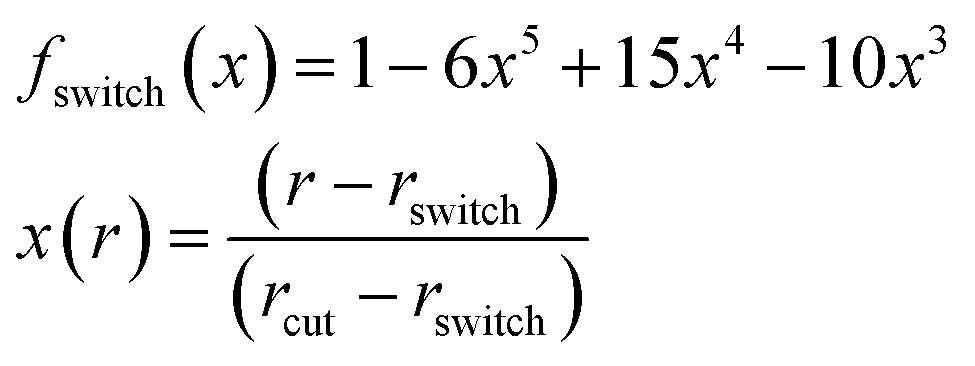
 employed a node-embedding and edge-embedding layer and message passing layers consisting of a single feed-forward layer of size 64. Each model was trained separately on its respective target. If not noted otherwise, models were optimized with Adam74 using an exponentially decaying learning rate ∈ [5 × 10⁻⁴, 1 × 10⁻⁵].